Article

Defect Detection in Atomic Resolution Transmission Electron Microscopy Images Using Machine Learning

1
Air Force Institute of Technology, Department of Mathematics & Statistics, 2950 Hobson Way, Wright-Patterson AFB, OH 45433, USA
2
Air Force Research Lab, Material and Manufacturing Directorate, Wright-Patterson AFB, OH 45433, USA
*
Authors to whom correspondence should be addressed.
Mathematics 2021, 9(11), 1209; https://doi.org/10.3390/math9111209
Submission received: 9 April 2021 / Revised: 20 May 2021 / Accepted: 24 May 2021 / Published: 27 May 2021
(This article belongs to the Special Issue Applied Mathematics and Computational Physics)

Abstract

:
Point defects play a fundamental role in the discovery of new materials due to their strong influence on material properties and behavior. At present, imaging techniques based on transmission electron microscopy (TEM) are widely employed for characterizing point defects in materials. However, current methods for defect detection predominantly involve visual inspection of TEM images, which is laborious and poses difficulties in materials where defect related contrast is weak or ambiguous. Recent efforts to develop machine learning methods for the detection of point defects in TEM images have focused on supervised methods that require labeled training data that is generated via simulation. Motivated by a desire for machine learning methods that can be trained on experimental data, we propose two self-supervised machine learning algorithms that are trained solely on images that are defect-free. Our proposed methods use principal components analysis (PCA) and convolutional neural networks (CNN) to analyze a TEM image and predict the location of a defect. Using simulated TEM images, we show that PCA can be used to accurately locate point defects in the case where there is no imaging noise. In the case where there is imaging noise, we show that incorporating a CNN dramatically improves model performance. Our models rely on a novel approach that uses the residual between a TEM image and its PCA reconstruction.

1. Introduction

Point defects are zero-dimensional defects in crystalline materials that have a strong influence on their atomic structure and properties. The engineering of point defects in materials, by creation of specific defect types and by the control of spatial location and number density, is foundational in the development of novel materials for advanced electronic and photonic applications. Transmission electron microscopy (TEM) is a widely used technique for imaging defects, due to its versatility for many different modes of imaging and spectroscopy at high spatial resolution. However, detection of point defects in TEM images continues to remain a challenge in many material systems, since the contrast due to the defect is affected by various factors such as its local environment and imaging conditions.
Recent efforts to develop machine learning methods for the detection of point defects in TEM images focused on supervised methods that require labeled training data that is generated via simulation. These methods treat the defect detection problem as a pixel-level classification problem [1,2]. In contrast, we treat the defect detection problem as an anomaly detection problem and propose two self-supervised machine learning methods that can be trained solely using defect-free TEM images. Importantly, since our models only require defect-free images for training, it allows for our models to be trained directly on experimental images of samples that are manufactured to be defect-free. The first method we propose uses principal components analysis (PCA) and the second method uses both PCA and convolutional neural networks (CNN). We assess the performance of these methods by introducing hypothetical anomalies that mimic point defects of different types in simulated images of defect-free GaAs (Figure 1) [3] and examining the detection accuracy of our proposed algorithms. We use GaAs as the test material. We also note that atomic resolution TEM imaging is performed in two different modes, wherein the electron beam is in parallel illumination (conventional high-resolution transmission electron microscopy) or as a focused probe (scanning transmission electron microscopy). The present work is based on parallel beam mode, since images simulated for this mode exhibits widely varying (although distinct) patterns for different imaging conditions, providing a large dataset for training and testing purposes. However, the results are also applicable to focused probe mode images.

Related Works

In recent years, CNNs have proven to be a highly effective tool for image analysis. Applications include image classification, object detection, pose estimation, and text recognition [4,5]. Given the data-intensive nature of TEM imagery, there have been recent efforts to employ CNNs in the analysis of TEM images. Examples of using neural networks for analyzing TEM images include using CNNs for denoising TEM images [6,7], generating TEM images from partial scans [8], enhancing TEM images [9,10], classifying types of crystalline structures [11], locating defects in non-crystalline materials [12], mapping atomic structures and defects [1], and mapping general structures of interest [2].
The latter two studies [1,2] are of particular interest because they propose CNN models that can be used to identify point defects in TEM images of crystalline materials. In both studies, the framework is to train a CNN using simulated TEM images and then apply the trained models to experimental images. Additionally, both propose training a multi-class classification CNN that outputs pixel-wise classifications, i.e., every pixel in a TEM image is assigned a predicted class. The classes can be vacancies, dopants, and defect-free lattice [1] or general, non-overlapping structural characteristics such as the column height of the sample [2]. Both of these models require extensive simulated data where the true label for each pixel is known. After training the pixel-wise classification model with pixel-by-pixel truth data, the models are shown to produce strong results on experimental TEM images.
Similar to the aforementioned work, we seek to develop a model that can detect local structures of interest in TEM images, namely defects, in crystalline materials. However, we choose to take an approach that does not rely on a training data set with pixel-by-pixel truth labels. Rather, we rely on a training set of TEM images that are only known to be free of defects. In both prior works, the authors acknowledge the difficulty in acquiring experimental images where the true defect locations are known and, therefore, propose models that are solely trained on simulated data with known defect locations. Since we only use a training set consisting of TEM images without defects, the proposed methods can be trained on simulated images or experimental images. Using TEM images of samples that are known to be free of defects, the proposed methods seek to locate areas of a TEM image that are anomalous and, thus, are most likely to contain a defect.
Due to a wide range of applications, anomaly detection has been well studied and there are numerous proposed anomaly detection techniques. Anomaly detection methods, also known as novelty detection methods, are trained using only “normal” observations and the goal is to accurately determine whether a new observation is anomalous or normal. Anomaly detection problems commonly arise in practice when there is an abundance of normal training data and a limited number of anomalous observations. Examples of well-known applications include medical imaging [13,14,15] and fraud detection [16,17,18]. A thorough review and taxonomy of machine learnings methods for anomaly is provided by Pimentel, et al. [19].
In recent years, CNNs have become a leading tool for anomaly detection in image data. Many of these efforts have been focused on benchmark datasets such as CIFAR-10 and ImageNet where the general approach is to use a subset of classes as normal data and then testing whether an image from a new class is correctly identified as an anomaly [20,21,22]. In this approach, a new image is considered an anomaly if the object in the new image does not match the objects included in the training data. For example, an anomaly detection model would attempt to distinguish between an airplane and a bird. One common framework for anomaly detection uses autoencoders to generate anomaly scores based on reconstruction error [23,24]. A thorough survey of deep learning methods for anomaly detection are provided in several works [25,26].
Defect detection can be considered a more specific type of anomaly detection problem where the goal is recognize subtle abnormalities in an image where the background object is normal. For example, a defect detection model would attempt to distinguish between a piece of fabric with and without a tear. While much progress has been made on general anomaly detection methods, recent work has shown that these methods do not generalize well to defect detection problems [27]. Tailored methods for defect detection [27,28] have been shown to outperform general anomaly detection models when using the MVTec benchmark dataset, a dataset specifically designed for defect detection [29]. Given that anomaly detection methods may generalize poorly to defect detection problems, our contribution is a novel method that is specifically intended for point defect detection in TEM images. While our methods are specifically tailored for defect detection in TEM images, our proposed PCA-CNN model has several parallels to recently proposed state-of-the-art defect detection methods [27].
In addition to our PCA-CNN model, we also propose a baseline defect detection method that uses principal components analysis (PCA) and reconstruction error to locate point defects in TEM images. The PCA model serves primarily as a performance baseline for the PCA-CNN model. PCA is a commonly used method for anomaly detection and is preferred for its simplicity [30,31,32]. PCA-based anomaly detection methods generally involve measuring the reconstruction error between a data point and its reconstruction. The reconstruction is generated via a linear transformation that is fitted on a training data set of normal observations [33]. The PCA method is presented in more detail in a later section. The concept of using reconstruction error for anomaly detection is also applicable to deep learning models that generate reconstructions via an autoencoder instead of PCA [20,23,24].

2. Materials and Methods

In this section, we introduce the simulated data used for model development and propose two methods for detecting defects in TEM images of GaAs. We specifically consider defect detection using high-resolution transmission electron microscopy (HRTEM) images, hereafter referred to as TEM images. The first method involves using PCA and reconstruction error, measured by mean squared error (MSE), to detect defects. The second method involves using PCA in combination with a weakly supervised CNN classification model to detect defects. Both models are trained using simulated TEM images of GaAs samples that are free of defects and then used to determine the location of a point defect in a simulated image of a GaAs sample. For each of the models, we consider the case when imaging noise is present and when there is no imaging noise.

2.1. Data Processing

The first step in developing a model for predicting the location of point defects is to generate simulated TEM images. We note that atomic resolution TEM imaging is performed in two different modes, wherein the electron beam is in parallel illumination (conventional high-resolution transmission electron microscopy) or as a focused probe (scanning transmission electron microscopy). The present work is based on parallel beam mode, since images simulated for this mode exhibits widely varying patterns for different imaging conditions, providing a large dataset for training and testing purposes. However, the results are also applicable to focused probe mode images. TEM images for GaAs were simulated using the TempasTM software. The TempasTM software has been developed in collaboration with the Material and Manufacturing Directorate, Air Force Research Lab (AFRL) and AFRL has validated the simulation results against experimental images of GaAs. The output of the simulation for a crystal projected along the [110] zone axis for TEM accelerating voltage of 300 kV and up to specimen thickness of 15 nm. The imaging parameters for the objective lens were set such that the spherical aberration coefficient was −15 μm and defocus ranging from −20 nm to +20 nm.
Ideally, experimental data would be used for this study, but due to the difficulty in acquiring experimental data, we use simulated TEM images to train and test our defect detection models. The use of simulated data is a start towards developing a method that can be trained directly on experimental data. A key consideration, then, is an understanding of the extent to which we can control defects in experimental images. As discussed earlier, it is possible to produce experimental GaAs samples that are defect-free so we assume it is feasible to acquire experimental TEM images that are known to be defect-free. In contrast, when defects, such as dopants, are added to experimental GaAs samples during the production process, the true locations of the dopant atoms in the GaAs sample are unknown. Thus, it is infeasible to generate a set of TEM images for which we know the true location of the point defects. The lack of knowledge about the true location of the defects in an experimental image is crucial. In light of this lack of defect truth data, the goal is to develop a defect detection method that is trained solely on defect-free TEM images.
Our dataset consists of simulated TEM images of GaAs using 8 different thickness conditions and 21 different defocus conditions. The thickness is varied from 1 nm to 15 nm in 2 nm steps. The defocus condition ranges from −20 nm to 20 nm in 2 nm steps. Thus, there are a total of 168 unique imaging conditions. These 168 imaging conditions are split into a set of 112 train conditions (66%) and 56 test conditions (33%). The splitting of the train and test conditions is done in a nonrandom manner. A third of the defocus conditions, {−18 nm, −12 nm, −6 nm, 0 nm, +6 nm, +12 nm, +18 nm}, are assigned to the test set and the remaining are assigned to the training set. The imaging conditions have a significant impact on the resulting TEM image so splitting on the imaging conditions ensures that model performance generalizes beyond conditions only in the set of training conditions. For the remainder of the paper, we refer to these sets as the train and test conditions.
We use the train and test conditions to further generate the training and tests data for our models. For each of the 112 train conditions, we simulate a single TEM image of dimension 1007 × 1024. The image is represented as a matrix of dimension 1007 × 1024 where each entry represents a grayscale pixel value. Since the TEM image consists of a repeating lattice structure, we choose to analyze the TEM images in smaller segments of dimension 84 × 118. Each of these image segments is large enough to include two sets of GaAs pairs in both the vertical and horizontal direction. At the same time, these image segments are small enough such that accurately identifying the presence of a defect in a particular image segment is nearly equivalent to determining the location of the defect. Thus, after generating the larger simulated TEM images, we generate 50 random crops from each training set image where each crop is an image segment of dimension 84 × 118. Please note that the crops are random so the location of the GaAs atoms differs within each image segment. These 5600 image segments constitute the training data for the PCA and form the basis for the training data for the CNN. During the training of the CNN, we apply data augmentation and randomized circular defects to the 5600 image segments to generate labeled training data. This process is described in more detail when we present the PCA-CNN model.
Next we use the test conditions to generate the test data. For each of the 56 test conditions, we generate 30 TEM images that are each 1007 × 1024. Specifically, each simulated image contains a single point defect that can be one of three defect types. For each of these three defect types, 10 replicates are generated where the defect location is randomized for each replicate. This results in a total of 1680 test images that are each 1007 × 1024. The three types of defects are (1) an antisite complex where the Gallium and Arsenic atoms are reversed, (2) substitutional defect where a dopant has an approximately 5% larger radius, (3) an arbitrary circular defect. 
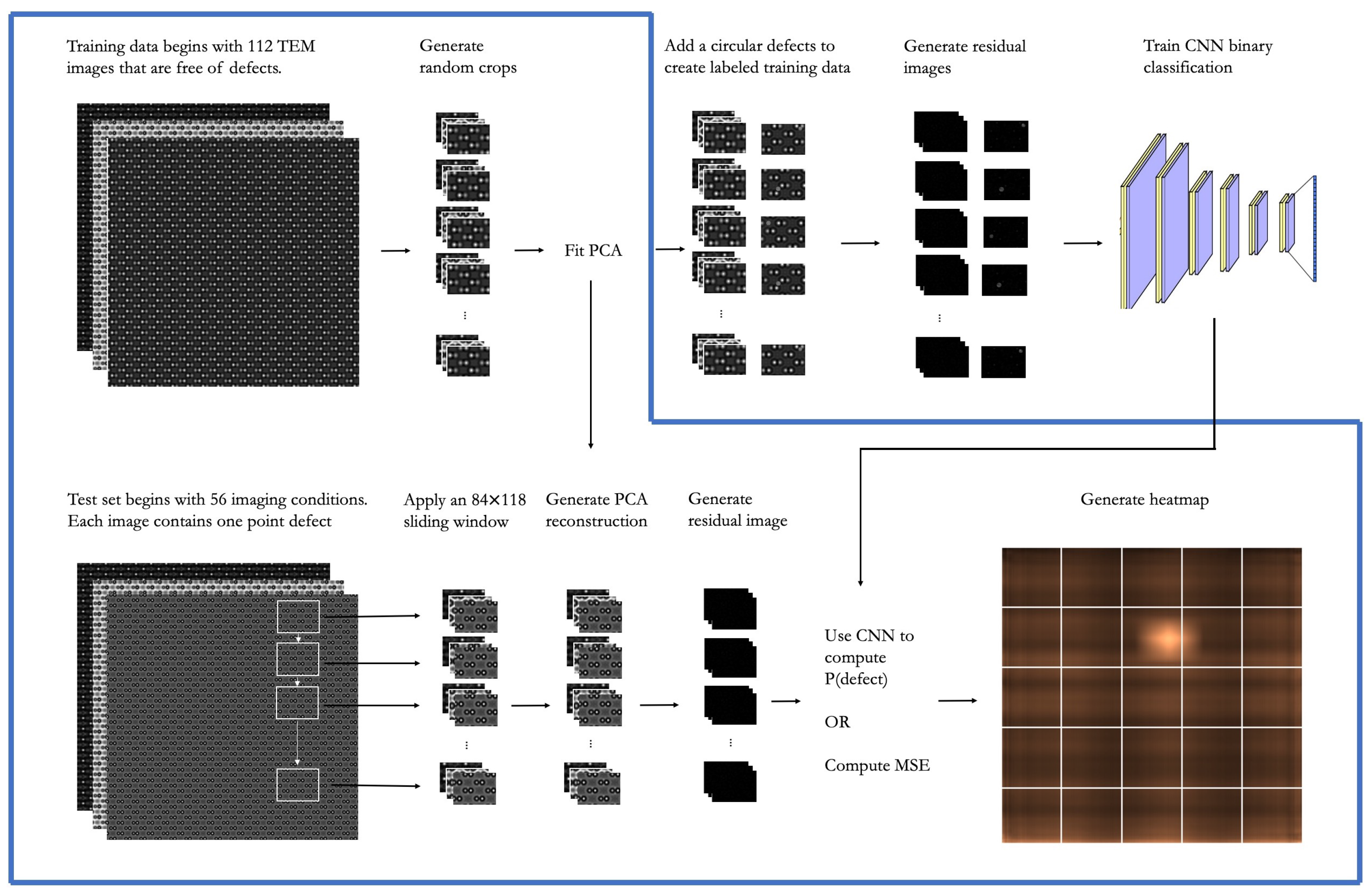
Figure 2a shows an example of each of the three defect types. We choose to consider these three types of defects because it includes a very subtle defect in the substitutional defect, a more obvious defect in the antisite defect, and a general defect in the circular defect. The circular defect is located randomly in an image segment while the other two located appropriately. The circular defect is meant to capture any general point defect such as an interstitial defect or a vacancy. The circular defect is unique in that it is easily added to any TEM image, either simulated or experimental. This flexibility plays an important role in the CNN model that introduced in a later section. For each combination of imaging condition and defect type, we generate 10 simulated TEM images with a randomly located defect. This results in 1680 test images where the defect location is known. Unlike the smaller image segments used in the training set, the images in the test set are 1007 × 1024. The test set images are used to evaluate whether or not the defect detection methods can accurately predict the location of the defect in the test image. Specifically, a 84 × 118 sliding window is used to determine the likelihood that each image segment in the 1007 × 1024 image contains a defect. Using a stride length of 4, each 1007 × 1024 image results in over 50,000 image segments that must be individually analyzed. The process for generating the training and test data is summarized in Figure 3.
The simulated TEM images do not include imaging noise. However, experimental TEM images can have varying degrees of noise that make it difficult to identify defects in a TEM image. Therefore, it is desirable for our proposed defect detection methods to be robust to imaging noise. To account for the presence of imaging noise in experimental images, Gaussian noise is used in both the training and test sets. Specifically, Gaussian noise with ε N ( μ = 0 , σ 2 = 0.05 ) is added to each pixel value for images in the training set. For the test set, varying levels of Gaussian noise, where σ2 = 0.00, 0.05, 0.10, are added to the TEM images and model performance is evaluated for each noise level. Figure 2b shows the effect of the Gaussian noise on a TEM image.

2.2. PCA Model

We present a method of detecting defects using PCA reconstructions. We fit a PCA transformation on the 5600 defect-free 84 × 118 image segments in the training set. Then we apply an 84 × 118 sliding window across each 1007 × 1024 test set image and, for each window, we generate a PCA reconstruction of the image segment in the window. Since the PCA transformation (and inverse transformation) is only fitted on defect-free TEM images, the assumption is that PCA will struggle to reconstruct an image with a defect. Thus, we expect that the reconstruction error of image segments with a defect to be greater than the reconstruction error of images without defects. We can predict the location of a defect by identifying the image segment with the highest MSE. With this framework in mind, we present the method in more detail below.
In general, PCA is a method for transforming a data matrix, X , with dimensions m × n to a lower-dimensional representation, X k , with dimensions m × k where k < n . Specifically, PCA involves a linear transformation, X k = X W k , where the transformation matrix is defined as W k = arg max W k X X k W k T with the constraint that W k is orthogonal, W k T W k = I . Notice that X k W k T is an m × n matrix that can be interpreted as a reconstruction of the original data using the lower-dimensional representation. Thus, W k is a transformation matrix that minimizes reconstruction error for a given data matrix X and dimension k [33].
In our PCA-based model, the training data consists of 50 randomly cropped image segments from each of the 112 larger TEM images in the training set. These 5600 training image segments can be represented by the data matrix Q R 5600 × 9912 where the rows represent individual image segments and the columns represent mean-centered values at each pixel location. The orthogonal linear transformation Q k = Q W k projects the original data, Q , to a lower k-dimensional representation, Q k . In PCA, the weight matrix W k R 9912 × k is constructed such that the reconstruction MSE, Q Q k W k T F 2 , is minimized. Notice that Q ^ = Q k W k T , a matrix of dimension 5600 × 9912 represents the reconstructed images. The projection to the lower-dimensional space and the reconstruction back to the original dimensional space are both determined by W k . Once W k is fit using the training data, it can be used to generate the reconstruction of any 84 × 118 image segment.
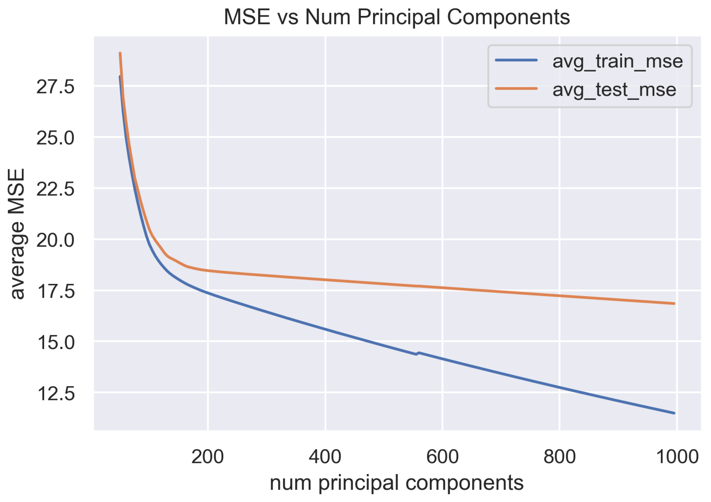
We set the value of k using reconstruction mean-squared error (MSE) of a test set. Specifically, we fit the PCA using the 5600 image segments in the training set and then apply the fitted PCA to image segment from the test conditions to compute the average reconstruction MSE. For each of the 56 test conditions, 50 random crops are taken where each crop is known to be free of defects. Figure 4 shows the effect of increasing the number of components on MSE. To prevent overfitting to the noise in the training set, we set k = 150 . Figure 4 shows several examples of image segments under various imaging conditions as well as the associated reconstruction with k = 150 . Figure 5 also shows examples of circular defects and the effect of the PCA reconstruction on the defect. The circular defects in the raw image are not visible in the PCA reconstruction which indicates that PCA reconstruction struggles to accurately reconstruct anomalous point defects.
The difference between an image segment and its reconstruction is referred to as the residual image. The residual image, intuitively, shows what is remaining when the general lattice structure is “subtracted” from the original image. Thus, the residual images consists of noise and any anomalies in the lattice structure. The reconstruction MSE can be regarded as a scalar that summarizes the residual image. For each of the 5600 images in the training set, we can compute the reconstruction MSE with and without a circular defect to understand the distribution of reconstruction MSE. Figure 6a shows how the presence of a defect changes the reconstruction MSE for each training example. In addition, Figure 6b shows how the addition of imaging noise affects the reconstruction MSE distribution with and without a defect. The concept of a residual image plays an important role in the CNN model that is presented in the next section.
After fitting the PCA transformation, we apply the resulting W k to the test set images via a sliding window. Recall that each test set image is of dimension 1007 × 1024 and contains a single point defect with known location. We use a 84 × 118 sliding window across the 1007 × 1024 image and, for each window, we complete the following three steps: (1) generate the PCA reconstruction, (2) generate the residual between the original image segment and the reconstruction, (3) compute the pixel-wise mean squared error (MSE). We then generate a heatmap that shows the average reconstruction MSE for each pixel in the full-size TEM image. The predicted location of the defect corresponds to the area of the heatmap that has the largest reconstruction MSE. Figure 7 shows an example of a test image and the corresponding MSE heatmap. The defect in the test image is a substitutional defect where a single Gallium atom is replaced with a dopant atom that has a 5% larger radius. The defect is difficult to identify visually, but the heatmap accurately locates the defect. This method is applied to all imaging conditions in the test set and we evaluate the accuracy in predicting the location of each type of defect. Figure 3 summarizes the process for predicting defect location using PCA.

2.3. PCA-CNN Model

In this section, we supplement the PCA-based detection method with a CNN classifier to improve the accuracy of the defect location predictions. This combined method significantly improves the prediction accuracy of the PCA model, especially in the case when there is imaging noise.
The PCA-based defect detection method has the benefit of being straightforward. However, in the presence of imaging noise, using PCA reconstruction error can lead to issues. Figure 5 shows the PCA residual images of segments with and without defects. In these particular examples, the reconstruction MSE for the defect images is actually lower than the reconstruction of the MSE for the defect-free images. Notably, if we visually inspect the residual images, the residual images clearly show the presence of a point defect. To address this shortcoming, we introduce a CNN classification model fitted on the PCA residual images. Intuitively, reconstruction MSE is equivalent to adding up the squared values in the residual image and it ignores any local patterns in the residual image. A CNN, on the other hand, can be trained to look for the presence of local patterns in the residual image that may be evidence of a defect. To the best of our knowledge, the use of the residual image for defect detection is a novel approach.
A CNN is a type of neural network that is commonly used for analyzing image data ([4]). The key concept in a CNN involves the use of small filters or kernels to extract local information from an image. A filter, often of dimension 3 × 3, is a matrix consisting of weights. The filter is applied to an image by sliding the filter across the image and taking the sum of the element-wise product between the filter weights and the image pixel values. The sums of these element-wise products are then stored in a new matrix, commonly referred to as a feature map, which can once again be analyzed using another set of filters. The training process of a CNN involves optimizing the filter weights to minimize a given loss function. In our application, our goal is to train a CNN to identify the presence of a defect within a residual image.
The training data for the CNN model begins with the same set of defect-free training images used to fit the PCA. Recall that 50 random crops from each of the 112 training images were used to fit the PCA. These same 5600 images are used to build a set of labeled training data for the CNN classifier. Since the training data only includes image segments that are defect-free, a set of labeled training data with defects is generated by adding random, circular defects to each of the 5600 training images. These circular defects could be representative of an interstitial defect or a vacancy, but they are not necessarily meant to represent a realistic defect that would be observed in an experimental image. Instead, the hope is that the CNN will learn to classify any residual image with an abnormal local pattern as one containing a defect. Since the circular defects are arbitrary and are added post-hoc to the simulated image, this method can easily be applied to experimental TEM images as well. After generating the labeled training, a CNN classification model is trained such that for an input PCA residual image, the model outputs a scalar y ^ = P ( defect ) where P ( defect ) [ 0 , 1 ] is the probability that the image segment contains a defect. A summary of the CNN model development process is visualized in Figure 3.
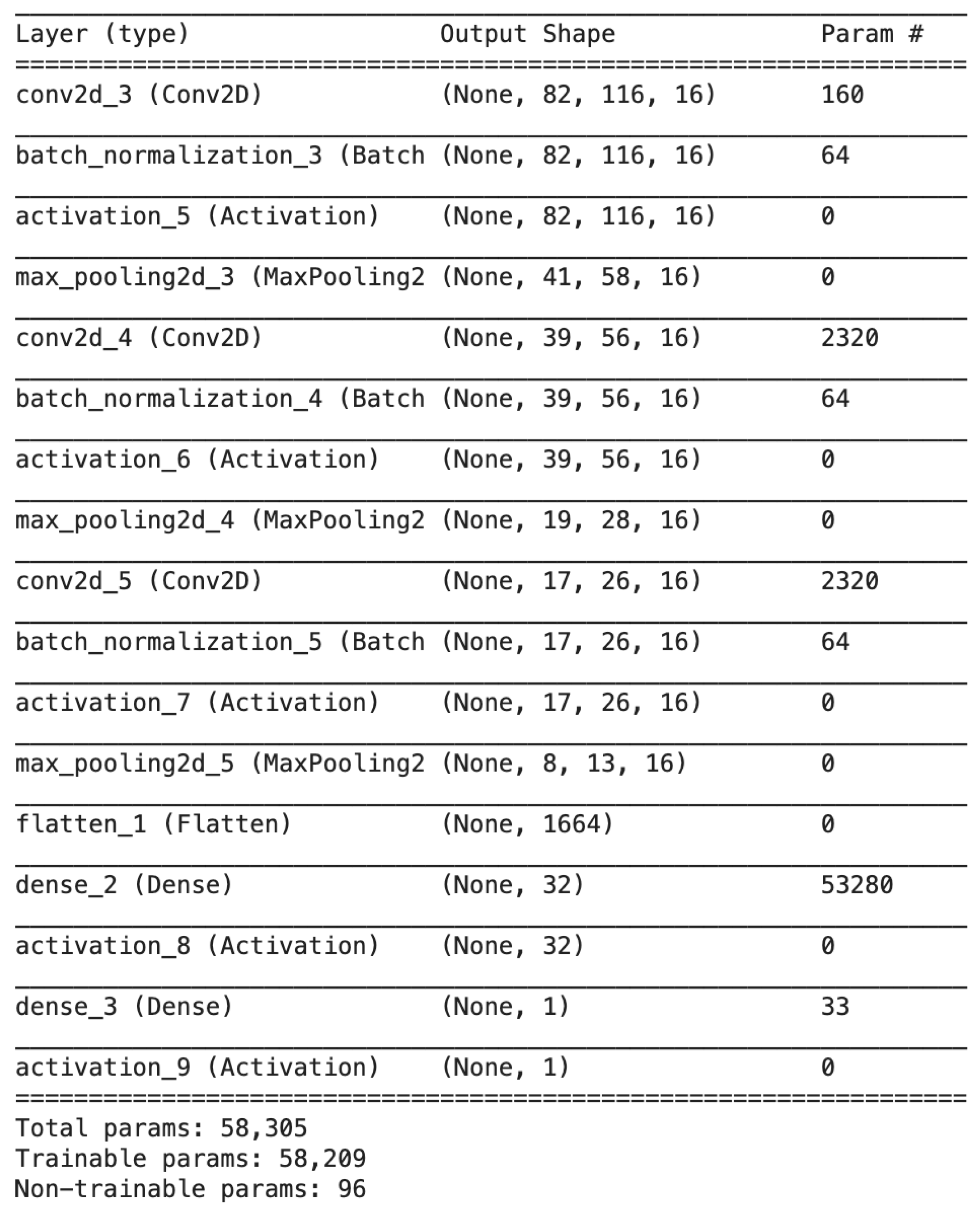
Our primary CNN architecture is adapted from the classic LeNet-5 architecture [34] and has 58,000 trainable parameters. Figure 8 shows the details of each layer of the CNN. It contains four convolutional layers with max-pooling following by two dense layers. We use a binary cross-entropy loss function and is optimized using nAdam. The model is trained for 200 epochs. Importantly, the training data are generated randomly for each batch so the location of the circular defects and noise patterns in the training set are randomized during training. The CNN is trained using Python 3.7 and Keras 2.3 with a TensorFlow 2.4.1 backend. The model achieves >99% training accuracy and test accuracy in less than 100 epochs. At the completion of 200 epochs, the test accuracy is 99.8% (Figure 9. Since the test set images are generated using a separate set of imaging conditions (focal length and thickness), the strong performance on the test set suggests that the trained CNN generalizes well to imaging conditions that were not included in the training set.
In addition to the LeNet based architecture, a VGG-16 architecture [35] was also implemented for comparison. The VGG-16 model was pretrained on ImageNet and the top dense layers were retrained using the TEM images. This resulted in 14.7 million fixed parameters and 3.2 million trainable parameters. After training for 100 epochs, the VGG-16 model achieved an accuracy of 98.2%. Given the much smaller size of the LeNet-based model and the better test set performance, the LeNet-based model was chosen as the preferred model.
After training the CNN, an 84 × 118 sliding window is applied to each of the 168 test images that are 1007 × 1024 with one hidden point defect. Using a stride of four pixels, this process results in 50,000 image segments that must be classified as having a defect or not. For each 84 × 118 window, we apply the following three steps: (1) generate a PCA reconstruction, (2) generate a residual image between the original image segment and the PCA reconstruction, and (3) pass the residual image into the trained CNN to generate P(defect). For each pixel in the 1007 × 1024 test image, we compute the average P(defect) for all sliding windows that contain the pixel. This results in a smoothed heatmap for the entire test image. The location of the defect is then predicted to be the area of the heatmap that has the highest average P(defect). The heatmap shown earlier in Figure 3 is an example of a heatmap generated using the CNN classification model with a sliding window.
In many applications of CNNs for anomaly detection, the output of the CNN classifier, P(defect), is compared to a fixed threshold value to determine if a particular input contains an anomaly or not [19]. Please note that a threshold is not necessary here since the predicted defect location is simply the pixel value with the largest average P(defect). If we generalize to the case where there are n defects in a GaAs sample, then the locations corresponding to the n largest average P(defect) would be the predicted locations of the defects.

3. Results

In this section, we compare the performance of the two defect detection methods discussed above. Recall that there are 56 imaging conditions that were reserved for the test set and there are three defect types. For each combination of imaging condition and defect type, we generate 10 simulated TEM images, each of dimension 1007 × 1024, where the defect location is randomized. This results in 1680 test images where the defect location is known. For each of the 1680 test images (540 images for each of the three defect types), we apply the PCA and PCA-CNN defect detection methods to predict the location of the defect. We compare the predicted defect location to the true defect location to determine whether the model successfully located the defect.
Table 1 shows the accuracy of both methods in predicting the defect location for various levels of imaging noise. The PCA defect detection method performs particularly well in the case of no imaging. It accurately locates all three defects types at nearly >97% and generally outperforms the CNN model. However, as the imaging noise increases, we observe the superior performance of the CNN model. Specifically, when imaging noise rises to σ 2 = 0.10 , the PCA model achieves an accuracy of 56% and 57% on antisite and circular defects, respectively, while the CNN model achieves 75% and 93% accuracy.
The results in Table 1a report the performance of the two methods under all test imaging conditions. Recall that the test set includes an equal number of TEM images for a range of defocus conditions. In practice, extreme defocus conditions are relatively uncommon and are actively avoided. Narrowing the focus on the central range of defocus conditions, {−6 nm, 0 nm, +6 nm}, provides a better representation of expected performance on experimental images. Table 1b shows the defect location accuracy of both methods under nominal defocus conditions. Under the restricted set of defocus conditions, the CNN model remains more robust in the presence of imaging noise. Specifically, when σ 2 = 0.10 , the CNN model achieves 89% and 91% accuracy for antisite and circular defects, respectively, while the PCA model achieves 70% and 61% accuracy.
Based on these preliminary results, it appears that the substitution defects are more challenging to identify compared to the antisite and circular defect. This is unsurprising given that the substitution defects are also the most challenging to identify from visual inspection. The substitution defects were purposely subtle so as to determine the effectiveness of the proposed methods for a wide range of defects. In practice, the substitution defects are unlikely to sit precisely in a gallium or arsenic site. If the substitution defect is slightly misaligned, then it is likely that the proposed methods would be more effective in locating the defect. The antisite and random circular defects are more readily identified visually which is reflected in the accuracy results. Although the circular defect is not representative of a particular defect, the circular defect could be representative of an interstitial defect or a vacancy.

4. Discussion

In this paper, we introduce two methods for determining the location of a point defect in a TEM image of GaAs. Compared to recent applications of using CNNs for defect detection ([1,2], and references therein), the proposed PCA and PCA-CNN methods of defect detection are unique in that they can be trained on TEM images that are defect-free. Unlike prior approaches to defect detection, this opens the door to training these models using experimental data. After training both models using a set of simulated images that are free of defects, we demonstrate the performance of both methods in locating a simulated defect in an HRTEM image. In the case of no imaging noise, we show the PCA method is sensitive to minor defects such as a subtle substitution defect (97% accuracy). However, as imaging noise is introduced, the performance of the PCA method declines rapidly. Supplementing the PCA method with a CNN classification model improves the performance of the model dramatically. The CNN classification model achieves >89% accuracy for both antisite and circular defects at the highest level of imaging noise ( σ 2 = 0.10 ). These results suggest that the CNN approach has the potential to be highly effective in analyzing experimental images.
Our PCA-CNN classification model is unique in that it is trained on PCA residual images. Using the PCA reconstruction to generate a residual image is a novel approach that has notable benefits. One of the benefits is that it allows for a single pre-trained CNN to be used for a wide range of imaging conditions. This is in contrast to prior studies that rely on condition-specific models for defect detection. Imaging conditions, such as thickness and defocus condition, change the overall “pattern” that is visible in an TEM image. By taking the difference between an image segment and its reconstruction, we are, intuitively, “subtracting” the pattern that is associated with a set of imaging conditions. The residual images are then less correlated with the imaging conditions used to generate the TEM image and can be analyzed using a single pre-trained CNN. Another benefit is that using the residual images allows a CNN to more effectively classify defects. Specifically, when we trained a CNN classification model directly on image segments in the training set without using residual images, the trained model far underperformed our model that uses residual images. This suggests that the use of residual images is a key step in training an effective CNN classification model in the context of TEM images.
The results presented in this paper are based on simulated TEM images. However, the goal is to implement and adapt these methods for experimental images as they become available. We observe that experimental images pose unique challenges compared to simulated images. In the simulated TEM images, the imaging conditions and the imaging noise were assumed to be consistent across the entire image. In contrast, the thickness of a sample can vary in an experimental image and the imaging noise is unlikely to be consistent across an entire image. While additional steps will be necessary to account for these variations, we believe the key ideas of using PCA reconstructions and residual images will remain an integral part of analyzing defects in experimental TEM images.

5. Conclusions

In this paper, we propose an anomaly detection method for locating point defects in crystalline materials using TEM images. The proposed method involves using a PCA reconstruction to generate a residual image and then a self-supervised CNN classifier to detect the presence of an anomaly in the residual image. Unlike earlier works that rely on extensive pixel-by-pixel labeled training data via simulation ([1,2]), our proposed method is a self-supervised method that only requires defect-free TEM images in the training set. Since the method only requires defect-free TEM images, it allows for the possibility of training a defect detection model directly on experimental TEM images that are defect-free. Additionally, our novel use of a residual image allows for strong results using a simple, computationally efficient CNN architecture that generalizes well to imaging conditions that are not included in the training set. Using simulated TEM images with a single point defect, we show that our PCA-CNN method is able to accurately locate point defects and it outperforms reconstruction error-based methods, particularly in the case when there is significant imaging noise.

Author Contributions

Conceptualization, P.C., A.W., K.M. and K.E.; methodology, P.C. and A.W.; software, P.C. and K.M.; investigation, P.C., A.W. and K.M.; formal analysis, P.C. and A.W.; investigation, P.C. and A.W.; writing—original draft preparation, P.C.; writing—review and editing, P.C., A.W., K.M. and K.E.; visualization, P.C.; supervision, A.W. All authors have read and agreed to the published version of the manuscript.

Funding

This research received no external funding.

Institutional Review Board Statement

Not applicable.

Informed Consent Statement

Not applicable.

Data Availability Statement

The simulated TEM images used in this study are being reviewed for public release by AFRL and are not currently available for public release. Individual data requests can be submitted to the corresponding author.

Conflicts of Interest

The authors declare no conflict of interest.

References

  1. Ziatdinov, M.; Dyck, O.; Maksov, A.; Li, X.; Sang, X.; Xiao, K.; Unocic, R.R.; Vasudevan, R.; Jesse, S.; Kalinin, S.V. Deep Learning of Atomically Resolved Scanning Transmission Electron Microscopy Images: Chemical Identification and Tracking Local Transformations. ACS Nano 2017, 11. [Google Scholar] [CrossRef] [PubMed] [Green Version]
  2. Madsen, J.; Liu, P.; Kling, J.; Wagner, J.B.; Hansen, T.W.; Winther, O.; Schiøtz, J. A Deep Learning Approach to Identify Local Structures in Atomic-Resolution Transmission Electron Microscopy Images. Adv. Theory Simul. 2018, 1. [Google Scholar] [CrossRef] [Green Version]
  3. Barron, A.; Raja, P.M.J. Crystal Structure. 2021. Available online: https://chem.libretexts.org/@go/page/55904 (accessed on 8 April 2021).
  4. Zhang, Q.; Zhang, M.; Chen, T.; Sun, Z.; Ma, Y.; Yu, B. Recent advances in convolutional neural network acceleration. Neurocomputing 2019, 323, 37–51. [Google Scholar] [CrossRef] [Green Version]
  5. Goodfellow, I.J.; Bengio, Y.; Courville, A. Deep Learning; MIT Press: Cambridge, MA, USA, 2016. [Google Scholar]
  6. Mohan, S.; Manzorro, R.; Vincent, J.L.; Tang, B.; Sheth, D.Y.; Simoncelli, E.P.; Matteson, D.S.; Crozier, P.A.; Fernandez-Granda, C. Deep Denoising For Scientific Discovery: A Case Study In Electron Microscopy. arXiv 2020, arXiv:2010.12970. [Google Scholar]
  7. Wang, F.; Henninen, T.R.; Keller, D.; Erni, R. Noise2Atom: Unsupervised denoising for scanning transmission electron microscopy images. Appl. Microsc. 2020. [Google Scholar] [CrossRef]
  8. Ede, J.M.; Beanland, R. Partial Scanning Transmission Electron Microscopy with Deep Learning. Sci. Rep. 2020, 10. [Google Scholar] [CrossRef] [PubMed]
  9. De Haan, K.; Ballard, Z.S.; Rivenson, Y.; Wu, Y.; Ozcan, A. Resolution enhancement in scanning electron microscopy using deep learning. Sci. Rep. 2019, 9, 1–7. [Google Scholar] [CrossRef] [PubMed]
  10. Suveer, A.; Gupta, A.; Kylberg, G.; Sintorn, I.M. Super-resolution reconstruction of transmission electron microscopy images using deep learning. In Proceedings of the 2019 IEEE 16th International Symposium on Biomedical Imaging (ISBI 2019), Venice, Italy, 8–11 April 2019. [Google Scholar] [CrossRef]
  11. Aguiar, J.A.; Gong, M.L.; Unocic, R.R.; Tasdizen, T.; Miller, B.D. Decoding crystallography from high-resolution electron imaging and diffraction datasets with deep learning. Sci. Adv. 2019, 5. [Google Scholar] [CrossRef] [PubMed] [Green Version]
  12. Li, W.; Field, K.G.; Morgan, D. Automated defect analysis in electron microscopic images. Npj Comput. Mater. 2018. [Google Scholar] [CrossRef] [Green Version]
  13. Clifton, L.; Clifton, D.A.; Watkinson, P.J.; Tarassenko, L. Identification of patient deterioration in vital-sign data using one-class support vector machines. In Proceedings of the 2011 Federated Conference on Computer Science and Information Systems, FedCSIS 2011, Szczecin, Poland, 18–21 September 2011. [Google Scholar]
  14. Quinn, J.A.; Williams, C.K. Known unknowns: Novelty detection in condition monitoring. In Lecture Notes in Computer Science (including Subseries Lecture Notes in Artificial Intelligence and Lecture Notes in Bioinformatics); Springer: Berlin/Heidelberg, Germany, 2007. [Google Scholar] [CrossRef] [Green Version]
  15. Tarassenko, L.; Hayton, P.; Cerneaz, N.; Brady, M. Novelty detection for the identification of masses in mammograms. In Proceedings of the 1995 Fourth International Conference on Artificial Neural Networks, Cambridge, UK, 26–28 June 1995. [Google Scholar] [CrossRef]
  16. Jyothsna, V.; Rama Prasad, V.; Munivara Prasad, K. A Review of Anomaly based Intrusion Detection Systems. Int. J. Comput. Appl. 2011. [Google Scholar] [CrossRef]
  17. Samrin, R.; Vasumathi, D. Review on anomaly based network intrusion detection system. In Proceedings of the 2017 International Conference on Electrical, Electronics, Communication, Computer, and Optimization Techniques (ICEECCOT), Mysuru, India, 15–16 December 2017. [Google Scholar] [CrossRef]
  18. Ganeshan, R.; Kolli, C.S.; Kumar, C.M.; Daniya, T. A Systematic Review on Anomaly Based Intrusion Detection System. In Proceedings of the IOP Conference Series: Materials Science and Engineering, Warangal, India, 9–10 October 2020. [Google Scholar] [CrossRef]
  19. Pimentel, M.A.; Clifton, D.A.; Clifton, L.; Tarassenko, L. A review of novelty detection. Signal Process. 2014, 99, 215–249. [Google Scholar] [CrossRef]
  20. Cho, P.; Farias, V.; Kessler, J.; Levi, R.; Magnanti, T.; Zarybnisky, E. Maintenance and flight scheduling of low observable aircraft. Nav. Res. Logist. 2015. [Google Scholar] [CrossRef]
  21. Ruff, L.; Vandermeulen, R.A.; Görnitz, N.; Deecke, L.; Siddiqui, S.A.; Binder, A.; Müller, E.; Kloft, M. Deep one-class classification. In Proceedings of the 35th International Conference on Machine Learning, ICML 2018, Stockholm, Sweden, 10–15 July 2018; Volume 10, pp. 6981–6996. [Google Scholar]
  22. Chalapathy, R.; Menon, A.K.; Chawla, S. Anomaly detection using one-class neural networks a preprint. arXiv 2018, arXiv:1802.06360. [Google Scholar]
  23. Thompson, B.B.; Marks, R.J.; Choi, J.J.; El-Sharkawi, M.A.; Huang, M.Y.; Bunje, C. Implicit learning in autoencoder novelty assessment. In Proceedings of the International Joint Conference on Neural Networks, Honolulu, HI, USA, 12–17 May 2002. [Google Scholar] [CrossRef]
  24. Hawkins, S.; He, H.; Williams, G.; Baxter, R. Outlier detection using replicator neural networks. In Lecture Notes in Computer Science (including Subseries Lecture Notes in Artificial Intelligence and Lecture Notes in Bioinformatics); Springer: Berlin/Heidelberg, Germany, 2002. [Google Scholar] [CrossRef]
  25. Pang, G.; Shen, C.; Cao, L.; van Den Hengel, A. Deep Learning for Anomaly Detection: A Review. arXiv 2020, arXiv:2007.02500. [Google Scholar]
  26. Chalapathy, R.; Chawla, S. Deep learning for anomaly detection: A survey. arXiv 2019, arXiv:1901.03407. [Google Scholar]
  27. Li, C.L.; Sohn, K.; Yoon, J.; Pfister, T. CutPaste: Self-Supervised Learning for Anomaly Detection and Localization. arXiv 2021, arXiv:2104.04015. [Google Scholar]
  28. Yi, J.; Yoon, S. Patch SVDD: Patch-Level SVDD for Anomaly Detection and Segmentation. In Lecture Notes in Computer Science (including Subseries Lecture Notes in Artificial Intelligence and Lecture Notes in Bioinformatics); Springer: Berlin/Heidelberg, Germany, 2020; pp. 375–390. [Google Scholar] [CrossRef]
  29. Bergmann, P. MVTec AD—A Comprehensive Real-World Dataset for Unsupervised Anomaly Detection. In Proceedings of the 2019 IEEE/CVF Conference on Computer Vision and Pattern Recognition (CVPR), Long Beach, CA, USA, 15–20 June 2019; pp. 9592–9600. [Google Scholar]
  30. Huang, L.; Nguyen, X.L.; Garofalakis, M.; Jordan, M.I.; Joseph, A.; Taft, N. In-network PCA and anomaly detection. In Advances in Neural Information Processing Systems; MIT Press: Cambridge, MA, USA, 2007. [Google Scholar] [CrossRef]
  31. Brauckhoff, D.; Salamatian, K.; May, M. Applying PCA for traffic anomaly detection: Problems and solutions. In Proceedings of the IEEE INFOCOM 2009, Rio de Janeiro, Brazil, 19–25 April 2009. [Google Scholar] [CrossRef] [Green Version]
  32. Jablonski, J.A.; Bihl, T.J.; Bauer, K.W. Principal Component Reconstruction Error for Hyperspectral Anomaly Detection. IEEE Geosci. Remote Sens. Lett. 2015. [Google Scholar] [CrossRef]
  33. Hastie, T.; Tibshirani, R.; Friedman, J. The Elements of Statistical Learning; Springer Series in Statistics; Springer: New York, NY, USA, 2001. [Google Scholar]
  34. LeCun, Y.; Bottou, L.; Bengio, Y.; Haffner, P. Gradient-based learning applied to document recognition. Proc. IEEE 1998, 86. [Google Scholar] [CrossRef] [Green Version]
  35. Simonyan, K.; Zisserman, A. Very deep convolutional networks for large-scale image recognition. In Proceedings of the 3rd International Conference on Learning Representations, ICLR 2015–Conference Track Proceedings, San Diego, CA, USA, 7–9 May 2015. [Google Scholar]
Figure 1. Examples of different types of defects that could occur. Green corresponds to A and red corresponds to B. Blue represents a dopant [3].
Mathematics 09 01209 g001
Figure 2. (a) Three different types of defects are considered. For each imaging condition in the test set, each of the three defect types is added to the test image. (b) Examples of increasing levels of Gaussian noise. The noise percentage level corresponds to the variance, σ2, of the Gaussian noise that is added the image. A circular defect is shown for reference.
Mathematics 09 01209 g002
Figure 3. The methodology of the PCA-based defect detection method is summarized by the steps bordered in blue. The steps outside the blue border are the additional necessary to incorporate the CNN classification model into the defect detection methodology.
Mathematics 09 01209 g003
Figure 4. The number of components used to fit the PCA is determined using the average reconstruction MSE of the test set images. The average reconstruction MSE for test set images falls rapidly and levels off after the number of components exceeds 150.
Mathematics 09 01209 g004
Figure 5. The first three rows show (1) the defect-free image segments with noise, (2) the PCA reconstruction, and (3) the residual between the raw and reconstructed image, respectively, for a range of imaging conditions. The bottom three rows show the same sequence images except the raw image contains a circular defect that has been randomly inserted. Notably, the PCA reconstructed image does not accurately reconstruct the defect since the PCA transformation was fitted only on images without defects.
Mathematics 09 01209 g005
Figure 6. The scatterplot shows the reconstruction MSE of 5600 defect-free image segments (x-axis) in the PCA training set and the corresponding reconstruction MSE for the same image segment with a circular defect inserted. Points that are close to the x = y represent image segments where the reconstruction MSE does not differ much with or without a defect. The marginal plots show the distribution of reconstruction MSEs with and without defects. On left, without imaging noise. On right, with imaging noise.
Mathematics 09 01209 g006
Figure 7. Heatmap that shows the pixels with the largest average MSE based on the PCA reconstruction. Bright spots correspond to areas that are mostly likely to have a defect.
Mathematics 09 01209 g007
Figure 8. CNN architecture motivated by LeNet-5.
Mathematics 09 01209 g008
Figure 9. Train and test set accuracy during the CNN training process. The input to the CNN model is a residual image of dimension 84 × 118 and the output is the probability that the image contains a defect, P(defect).
Mathematics 09 01209 g009
Table 1. Accuracy of the PCA and PCA-CNN model in locating point defects in the test set images. Table (a) shows the accuracy results when including all images in the test set. Table (b) shows the accuracy results when only the nominal defocus conditions are included. In both cases, the CNN model is more robust to imaging noise.
(a) Location detection accuracy including all imaging conditions
MethodNoiseSubstitution
n = 560
Antisite
n = 560
Circular
n = 560
PCA σ 2 = 0.000.971.001.00
σ 2 = 0.050.160.800.94
σ 2 = 0.100.040.560.57
PCA-CNN σ 2 =0.000.710.861.00
σ 2 = 0.050.640.900.99
σ 2 = 0.100.140.750.93
(b) Location detection accuracy for central defocus conditions, {−6 nm, 0 nm, +6 nm}
MethodNoiseSubstitution
n = 240
Antisite
n = 240
Circular
n = 240
PCA σ 2 = 0.001.001.001.00
σ 2 = 0.050.240.910.92
σ 2 = 0.100.040.700.61
PCA-CNN σ 2 = 0.001.000.981.00
σ 2 = 0.050.890.990.99
σ 2 = 0.100.230.890.91
Publisher’s Note: MDPI stays neutral with regard to jurisdictional claims in published maps and institutional affiliations.

