A Conservative and Implicit Second-Order Nonlinear Numerical Scheme for the Rosenau-KdV Equation

Abstract

In this paper, for solving the nonlinear Rosenau-KdV equation, a conservative implicit two-level nonlinear scheme is proposed by a new numerical method named the multiple integral finite volume method. According to the order of the original differential equation’s highest derivative, we can confirm the number of integration steps, which is just called multiple integration. By multiple integration, a partial differential equation can be converted into a pure integral equation. This is very important because we can effectively avoid the large errors caused by directly approximating the derivative of the original differential equation using the finite difference method. We use the multiple integral finite volume method in the spatial direction and use finite difference in the time direction to construct the numerical scheme. The precision of this scheme is $O({\tau }^2+h^3)$. In addition, we verify that the scheme possesses the conservative property on the original equation. The solvability, uniqueness, convergence, and unconditional stability of this scheme are also demonstrated. The numerical results show that this method can obtain highly accurate solutions. Further, the tendency of the numerical results is consistent with the tendency of the analytical results. This shows that the discrete scheme is effective.

1. Introduction

Proposed by Korteweg and de Vries, the Korteweg–de Vries (KdV) equation,

$$u_t+u{u}_x+u_{xxx}=0$$

(1)

has been widely studied. It can describe ion–phonon waves, magnetic fluid waves in cold plasma, unidirectional shallow water waves with small amplitude and long waves, and other wave processes in some physical and biological systems.

It has a wide range of physical applications, so there is great interest in this equation. A great many numerical methods have been proposed to obtain the numerical solutions of KdV equations [1,2,3,4,5]. In addition, [6] developed a new integral equation using the negative-order KdV equation and derived multiple soliton solutions, while [7] created various negative-order KdV equations in (3 + 1) dimensions and discussed the solutions for each derived model.

Given the shortcomings of the KdV equation in describing wave–wave and wave–wall interactions, Rosenau [8,9] proposed the Rosenau equation to cope with the compact discrete dynamic system.

$$u_t+u_{xxxxt}+u_x+u{u}_x=0$$

(2)

The existence, uniqueness, and regularity of solutions were derived by Park [10]. Since then, several numerical methods have been studied for the Rosenau equation. For example, ref [11] used the Petviashvili iteration method to construct numerical solitary wave solutions; ref [12] applied Galerkin mixed finite element methods to (2) by employing a splitting technique; ref [13] discussed new methods to expand solutions for wave equations like Rosenau-type equations with damping terms; ref [14] constructed an implicit Crank–Nicolson formula of the mixed finite element method for nonlinear fourth-order Rosenau equations; and [15] proposed a meshfree method based on the radial basis function for the Rosenau equation and other higher-order partial differential equations(PDEs). The long-time behavior of solutions was investigated in [16].

To better study nonlinear waves, the viscous term $u_{xxx}$ needs to be included.

$$u_t+u_{xxxxt}+u_x+u{u}_x+u_{xxx}=0$$

(3)

Equation (3) is usually called the Rosenau-KdV equation. The authors of [17,18] proposed conservative schemes for the Rosenau-KdV equation based on the finite difference method. The authors of [19] proposed a Crank–Nicolson meshless spectral radial point interpolation (CN-MSRPI) method for the nonlinear Rosenau-KdV equation. The authors of [20] solved the equation by the first-order Lie–Trotter and second-order Strang time-splitting techniques combined with quintic B-spline collocation, while [21] studied numerical solutions by using the subdomain method based on sextic B-spline basis functions. Although various methods have been proposed, we wonder whether there might be a new method with higher accuracy and efficiency that can keep some properties of the original partial differential equation. Further, research on the Rosenau-KdV equation under certain conditions is relatively lacking.

In this paper, we consider the Rosenau-KdV Equation (4) with initial condition

$$u\left(x,0\right)=u_0\left(x\right), x\in [x_l,x_r]$$

(4)

and boundary conditions

$$u\left(x_l,t\right)=u\left(x_r,t\right)=0, u_x\left(x_l,t\right)=u_x\left(x_r,t\right)=0, t\in [0,T]$$

(5)

Here, $u_0\left(x\right)$ is a known smooth function, and $x_l$ and $x_r$ are, respectively, the left border and the right border of $x$.

Theorem 1.

The system (3)–(5) satisfies the following conservative property:

$$E\left(t\right)={\Vert u\Vert }_{L^2}^2+{\Vert u_{xx}\Vert }_{L^2}^2=E\left(0\right)=\mathit{Const}.$$

(6)

Here, ${\Vert u \Vert }_{L^2}^2={\displaystyle \underset{x_l}{\overset{x_r}{\int }}{u}^2 }dx$.

Proof. 

Integrate both sides of Equation (3) from $x_l$ to $x_r$ and apply (5); we thus obtain

$${\displaystyle \underset{x_l}{\overset{x_r}{\int }}\left(u_t+u_{xxxxt}+u_{xx}+u_x+u{u}_x\right)u }dx=\frac{1}{2}\frac{\partial }{\partial t}\left({\Vert u \Vert }_{L^2}^2+{\Vert u_{xx}\Vert }_{L^2}^2\right)=0$$

(7)

Let $E\left(t\right)={\Vert u\Vert }_{L^2}^2+{\Vert u_{xx}\Vert }_{L^2}^2$. Then we get

$$E\left(t\right)={\Vert u\Vert }_{L^2}^2+{\Vert u_{xx}\Vert }_{L^2}^2=E\left(0\right)=\mathit{Const}.$$

(8)

Hence, the system (3)–(5) meets the conservative property. □

In this paper, we present a two-level implicit nonlinear discrete scheme for the Rosenau-KdV Equations (3)–(5) by using a new method named the multiple integral finite volume method (MIFVM). The remaining contents of this paper are arranged as follows: In Section 2, we introduce MIFVM in detail and propose a numerical scheme. The conservative property of this scheme is also discussed. In Section 3, the solvability of this numerical scheme is derived. Then, in Section 4, we show some prior estimates. According to the prior estimates, we demonstrate the convergence with order $O({\tau }^2+h^3)$ and unconditional stability of this numerical scheme in Section 5. In Section 6, the uniqueness of this numerical solution is verified with the classic theorem. Finally, we verify the effectiveness of the numerical scheme via some numerical experiments in Section 7.

2. A Two-Level Implicit Nonlinear Discrete Scheme and Its Conservative Law

2.1. Notation

Let $h$ and $\tau$ be uniform step sizes in the spatial and temporal directions, respectively. Let $x_j=x_l+jh\left(j=0,1,\cdots ,J\right)$, $t_n=n\tau \left(n=0,1,\cdots ,N\right)$, where $h=\left(x_r-x_l\right)/J$, $\tau =T/N$. Further, let $u_j=u_j(t)=u(x_l+jh,t)$, $u_j^n=u(x_l+jh,t_n)$, $Z_h^0=\left\{u_j\right|u_0=u_J=0,j=0,1,\cdots ,J\}$, and ${\Omega }_h=\left\{x_j|j=0,1,\cdots ,J\right\}$. In this paper, we let $C$ denote a generic positive constant independent of $h$ and $\tau$. The difference operators, inner product, and norms we defined are shown below.

$$\begin{array}{c}{u}_j^{n+\frac{1}{2}}=\frac{u_j^{n+1}+u_j^n}{2}{\left(u_j^n\right)}_x=\frac{u_{j+1}^n-u_j^n}{h}, {\left(u_j^n\right)}_{\overline{x}}=\frac{u_j^n-u_{j-1}^n}{h}, {\left(u_j^n\right)}_{\widehat{x}}=\frac{u_{j+1}^n-u_{j-1}^n}{2h},\\ {\left(u_j^n\right)}_{x\overline{x}}={\left(u_j^n\right)}_{\overline{x}x}=\frac{u_{j+1}^n-2u_j^n+u_{j-1}^n}{h^2}, {\left(u_j^n\right)}_{x\overline{x}\widehat{x}}=\frac{u_{j+2}^n-2u_{j+1}^n+2u_{j-1}^n-u_{j-2}^n}{2h^3},\\ {\left(u_j^n\right)}_{xx\overline{x}\overline{x}}=\frac{u_{j+2}^n-4u_{j+1}^n+6u_j^n-4u_{j-1}^n+u_{j-2}^n}{h^4}, {\left(u_j^{n+\frac{1}{2}}\right)}_{\widehat{t}}=\frac{u_j^{n+1}-u_j^n}{\tau },\\ \Vert u^n\Vert =\sqrt{(u^n,u^n)}, {\Vert u^n\Vert }_{\infty }=\underset{x_j\in {\Omega }_h}{\max }\left|u_j^n\right|, (u^n,v^n)={\displaystyle \sum _{j=0}^J{u}_j^n{v}_j^n}h\end{array}$$

However, we should note that if the inner product operates on different functions, there will be different ranges of values of j, for example, $(u_x^n,v_x^n)={\displaystyle \sum _{j=0}^{J-1}{\left(u_j^n\right)}_x{\left(v_j^n\right)}_{x}h}$ and $(u_{\overline{x}}^n,v_{\overline{x}}^n)={\displaystyle \sum _{j=1}^J{\left(u_j^n\right)}_{\overline{x}}{\left(v_j^n\right)}_{\overline{x}}h}$.

Lemma 1.

For any two mesh functions$u, v\in Z_h^0$, the following equations hold.

$$\left(u_x,v\right)=-\left(u,v_{\overline{x}}\right),\left(u_{x\overline{x}},v\right)=-\left(u_x,v_x\right) ,\left(u_{\widehat{x}},v\right)=-\left(u,v_{\widehat{x}}\right)$$

Furthermore, if ${\left(u_0^n\right)}_{x\overline{x}}={\left(u_J^n\right)}_{x\overline{x}}=0$, then $\left({\left(u^n\right)}_{xx\overline{x} \overline{x}},u^n\right)={\Vert u_{xx}^n\Vert }^2$.

Lemma 2.

For any mesh function$u\in Z_h^0$, the following equation holds.

$${\Vert u_{\widehat{x}}\Vert }^2\le {\Vert u_x\Vert }^2$$

(9)

Lemma 3.

For any discrete function$u\in Z_h^0$, we have

$$\left(\phi (u),u\right)={\displaystyle \sum _{j=1}^{J-1}\frac{1}{3}{\left(u_j^{}\right)}_{\widehat{x}}\left(u_{j-1}^{}+u_j^{}+u_{j+1}^{}\right)u_j^{}}h=0,$$

(10)

where$\phi (u_j)=\frac{1}{3}{\left(u_j^{}\right)}_{\widehat{x}}\left(u_{j-1}^{}+u_j^{}+u_{j+1}^{}\right)$.

Proof. 

Because $u\in Z_h^0$, we have

$$\begin{array}{ll}\left(\phi (u),u\right)& =\frac{1}{6h}{\displaystyle \sum _{j=1}^{J-1}\left[u_{j+1}^{}{u}_j^{}-u_j^{}{u}_{j-1}^{}+{\left(u_{j+1}^{}\right)}^2-{\left(u_{j-1}^{}\right)}^2\right]u_j^{}}\\ & =\frac{1}{6h}\left[{\displaystyle \sum _{j=1}^{J-2}\left(u_j^{}+u_{j+1}^{}\right)u_j^{}{u}_{j+1}^{}}-{\displaystyle \sum _{j=2}^{J-1}\left(u_{j-1}^{}+u_j^{}\right)u_{j-1}^{}{u}_j^{}}\right]=0\end{array}$$

(11)

□

2.2. The Multiple Integral Finite Volume Method(MIFVM)

In this paper, we use a method named MIFVM to construct a two-level implicit nonlinear scheme for the Rosenau-KdV Equations (3)–(5).The method uses multiple integrals and combines the finite difference method with the finite volume method. We thus discretize the original PDE into separate spatial and temporal directions.

In the spatial $x$ direction, firstly, by multiple integrals, we turn the original differential Equation (3), with unknown function $u$ and its derivative, into an integral equation with only the unknown function. This is very important because we can effectively avoid the large errors caused by directly approximating the derivative of the original differential equation using the finite difference method. We use the multiple integral finite volume method in the spatial direction and use finite difference in the time direction to construct the numerical scheme. Firstly, in the spatial direction, the number of integration steps $m$ depends on the order of the highest derivative in the $x$ direction of the original PDE. Considering the original Equation (3), the order of the highest derivative in the $x$ direction is four, so $m=2^4-1=15$. Now, we define a 15-time integral,

$$\begin{array}{ll}{\displaystyle \underset{xxxx}{\int }u}={\displaystyle \underset{xxxx}{\int }u\left(x,t\right) }\underset{\_}{\underset{\_}{def}}& {\displaystyle \underset{x_j+{\epsilon }_7}{\overset{x_j+{\epsilon }_8}{\int }}d{x}_{f_2}}{\displaystyle \underset{x_j+{\epsilon }_6}{\overset{x_j+{\epsilon }_7}{\int }}d{x}_{f_1}}{\displaystyle \underset{x_j+{\epsilon }_5}{\overset{x_j+{\epsilon }_6}{\int }}d{x}_{e_2}}{\displaystyle \underset{x_j}{\overset{x_j+{\epsilon }_5}{\int }}d{x}_{e_1}}{\displaystyle \underset{x_j-{\epsilon }_4}{\overset{x_j}{\int }}d{x}_{d_2}}\\ & {\displaystyle \underset{x_j-{\epsilon }_3}{\overset{x_j-{\epsilon }_4}{\int }}d{x}_{d_1}}{\displaystyle \underset{x_j-{\epsilon }_2}{\overset{x_j-{\epsilon }_3}{\int }}d{x}_{c_2}}{\displaystyle \underset{x_j-{\epsilon }_1}{\overset{x_j-{\epsilon }_2}{\int }}d{x}_{c_1}}{\displaystyle \underset{x_{f_1}}{\overset{x_{f_2}}{\int }}d{x}_f} {\displaystyle \underset{x_{e_1}}{\overset{x_{e_2}}{\int }}d{x}_e}{\displaystyle \underset{x_{d_1}}{\overset{x_{d_2}}{\int }}d{x}_d}\\ & {\displaystyle \underset{x_{c_1}}{\overset{x_{c_2}}{\int }}d{x}_c}{\displaystyle \underset{x_e}{\overset{x_f}{\int }}d{x}_b}{\displaystyle \underset{x_c}{\overset{x_d}{\int }}d{x}_a}{\displaystyle \underset{x_a}{\overset{x_b}{\int }}u(x,t) dx}\end{array}$$

(12)

and we treat original Equation (2) using integral (12). Then, we can get

$$\begin{array}{l}{\displaystyle \underset{x_j+{\epsilon }_7}{\overset{x_j+{\epsilon }_8}{\int }}d{x}_{f_2}}{\displaystyle \underset{x_j+{\epsilon }_6}{\overset{x_j+{\epsilon }_7}{\int }}d{x}_{f_1}}{\displaystyle \underset{x_j+{\epsilon }_5}{\overset{x_j+{\epsilon }_6}{\int }}d{x}_{e_2}}{\displaystyle \underset{x_j}{\overset{x_j+{\epsilon }_5}{\int }}d{x}_{e_1}}{\displaystyle \underset{x_j-{\epsilon }_4}{\overset{x_j}{\int }}d{x}_{d_2}}{\displaystyle \underset{x_j-{\epsilon }_3}{\overset{x_j-{\epsilon }_4}{\int }}d{x}_{d_1}}{\displaystyle \underset{x_j-{\epsilon }_2}{\overset{x_j-{\epsilon }_3}{\int }}d{x}_{c_2}}\\ {\displaystyle \underset{x_j-{\epsilon }_1}{\overset{x_j-{\epsilon }_2}{\int }}d{x}_{c_1}}{\displaystyle \underset{x_{f_1}}{\overset{x_{f_2}}{\int }}d{x}_f}{\displaystyle \underset{x_{e_1}}{\overset{x_{e_2}}{\int }}d{x}_e}{\displaystyle \underset{x_{d_1}}{\overset{x_{d_2}}{\int }}d{x}_d}{\displaystyle \underset{x_{c_1}}{\overset{x_{c_2}}{\int }}d{x}_c}{\displaystyle \underset{x_e}{\overset{x_f}{\int }}d{x}_b}{\displaystyle \underset{x_c}{\overset{x_d}{\int }}d{x}_a}{\displaystyle \underset{x_a}{\overset{x_b}{\int }}{u}_t dx}\\ +{\displaystyle \underset{x_j+{\epsilon }_7}{\overset{x_j+{\epsilon }_8}{\int }}d{x}_{f_2}}{\displaystyle \underset{x_j+{\epsilon }_6}{\overset{x_j+{\epsilon }_7}{\int }}d{x}_{f_1}}{\displaystyle \underset{x_j+{\epsilon }_5}{\overset{x_j+{\epsilon }_6}{\int }}d{x}_{e_2}}{\displaystyle \underset{x_j}{\overset{x_j+{\epsilon }_5}{\int }}d{x}_{e_1}}{\displaystyle \underset{x_j-{\epsilon }_4}{\overset{x_j}{\int }}d{x}_{d_2}}{\displaystyle \underset{x_j-{\epsilon }_3}{\overset{x_j-{\epsilon }_4}{\int }}d{x}_{d_1}}{\displaystyle \underset{x_j-{\epsilon }_2}{\overset{x_j-{\epsilon }_3}{\int }}d{x}_{c_2}}\\ {\displaystyle \underset{x_j-{\epsilon }_1}{\overset{x_j-{\epsilon }_2}{\int }}d{x}_{c_1}}{\displaystyle \underset{x_{f_1}}{\overset{x_{f_2}}{\int }}d{x}_f}{\displaystyle \underset{x_{e_1}}{\overset{x_{e_2}}{\int }}d{x}_e}{\displaystyle \underset{x_{d_1}}{\overset{x_{d_2}}{\int }}d{x}_d}{\displaystyle \underset{x_{c_1}}{\overset{x_{c_2}}{\int }}d{x}_c}{\displaystyle \underset{x_e}{\overset{x_f}{\int }}d{x}_b}{\displaystyle \underset{x_c}{\overset{x_d}{\int }}d{x}_a}{\displaystyle \underset{x_a}{\overset{x_b}{\int }}{u}_{xxxxt} dx}\\ +{\displaystyle \underset{x_j+{\epsilon }_7}{\overset{x_j+{\epsilon }_8}{\int }}d{x}_{f_2}}{\displaystyle \underset{x_j+{\epsilon }_6}{\overset{x_j+{\epsilon }_7}{\int }}d{x}_{f_1}}{\displaystyle \underset{x_j+{\epsilon }_5}{\overset{x_j+{\epsilon }_6}{\int }}d{x}_{e_2}}{\displaystyle \underset{x_j}{\overset{x_j+{\epsilon }_5}{\int }}d{x}_{e_1}}{\displaystyle \underset{x_j-{\epsilon }_4}{\overset{x_j}{\int }}d{x}_{d_2}}{\displaystyle \underset{x_j-{\epsilon }_3}{\overset{x_j-{\epsilon }_4}{\int }}d{x}_{d_1}}{\displaystyle \underset{x_j-{\epsilon }_2}{\overset{x_j-{\epsilon }_3}{\int }}d{x}_{c_2}}\\ {\displaystyle \underset{x_j-{\epsilon }_1}{\overset{x_j-{\epsilon }_2}{\int }}d{x}_{c_1}}{\displaystyle \underset{x_{f_1}}{\overset{x_{f_2}}{\int }}d{x}_f}{\displaystyle \underset{x_{e_1}}{\overset{x_{e_2}}{\int }}d{x}_e}{\displaystyle \underset{x_{d_1}}{\overset{x_{d_2}}{\int }}d{x}_d}{\displaystyle \underset{x_{c_1}}{\overset{x_{c_2}}{\int }}d{x}_c}{\displaystyle \underset{x_e}{\overset{x_f}{\int }}d{x}_b}{\displaystyle \underset{x_c}{\overset{x_d}{\int }}d{x}_a}{\displaystyle \underset{x_a}{\overset{x_b}{\int }}{u}_x dx}\\ +{\displaystyle \underset{x_j+{\epsilon }_7}{\overset{x_j+{\epsilon }_8}{\int }}d{x}_{f_2}}{\displaystyle \underset{x_j+{\epsilon }_6}{\overset{x_j+{\epsilon }_7}{\int }}d{x}_{f_1}}{\displaystyle \underset{x_j+{\epsilon }_5}{\overset{x_j+{\epsilon }_6}{\int }}d{x}_{e_2}}{\displaystyle \underset{x_j}{\overset{x_j+{\epsilon }_5}{\int }}d{x}_{e_1}}{\displaystyle \underset{x_j-{\epsilon }_4}{\overset{x_j}{\int }}d{x}_{d_2}}{\displaystyle \underset{x_j-{\epsilon }_3}{\overset{x_j-{\epsilon }_4}{\int }}d{x}_{d_1}}{\displaystyle \underset{x_j-{\epsilon }_2}{\overset{x_j-{\epsilon }_3}{\int }}d{x}_{c_2}}\\ {\displaystyle \underset{x_j-{\epsilon }_1}{\overset{x_j-{\epsilon }_2}{\int }}d{x}_{c_1}}{\displaystyle \underset{x_{f_1}}{\overset{x_{f_2}}{\int }}d{x}_f}{\displaystyle \underset{x_{e_1}}{\overset{x_{e_2}}{\int }}d{x}_e}{\displaystyle \underset{x_{d_1}}{\overset{x_{d_2}}{\int }}d{x}_d}{\displaystyle \underset{x_{c_1}}{\overset{x_{c_2}}{\int }}d{x}_c}{\displaystyle \underset{x_e}{\overset{x_f}{\int }}d{x}_b}{\displaystyle \underset{x_c}{\overset{x_d}{\int }}d{x}_a}{\displaystyle \underset{x_a}{\overset{x_b}{\int }}u{u}_x dx}\\ +{\displaystyle \underset{x_j+{\epsilon }_7}{\overset{x_j+{\epsilon }_8}{\int }}d{x}_{f_2}}{\displaystyle \underset{x_j+{\epsilon }_6}{\overset{x_j+{\epsilon }_7}{\int }}d{x}_{f_1}}{\displaystyle \underset{x_j+{\epsilon }_5}{\overset{x_j+{\epsilon }_6}{\int }}d{x}_{e_2}}{\displaystyle \underset{x_j}{\overset{x_j+{\epsilon }_5}{\int }}d{x}_{e_1}}{\displaystyle \underset{x_j-{\epsilon }_4}{\overset{x_j}{\int }}d{x}_{d_2}}{\displaystyle \underset{x_j-{\epsilon }_3}{\overset{x_j-{\epsilon }_4}{\int }}d{x}_{d_1}}{\displaystyle \underset{x_j-{\epsilon }_2}{\overset{x_j-{\epsilon }_3}{\int }}d{x}_{c_2}}\\ {\displaystyle \underset{x_j-{\epsilon }_1}{\overset{x_j-{\epsilon }_2}{\int }}d{x}_{c_1}}{\displaystyle \underset{x_{f_1}}{\overset{x_{f_2}}{\int }}d{x}_f}{\displaystyle \underset{x_{e_1}}{\overset{x_{e_2}}{\int }}d{x}_e}{\displaystyle \underset{x_{d_1}}{\overset{x_{d_2}}{\int }}d{x}_d}{\displaystyle \underset{x_{c_1}}{\overset{x_{c_2}}{\int }}d{x}_c}{\displaystyle \underset{x_e}{\overset{x_f}{\int }}d{x}_b}{\displaystyle \underset{x_c}{\overset{x_d}{\int }}d{x}_a}{\displaystyle \underset{x_a}{\overset{x_b}{\int }}{u}_{xxx} dx}=0 \end{array}$$

(13)

We then use Lagrange interpolation to approximate $u(x_j\pm {\epsilon }_i,t)(i=1,2,\cdots ,8)$, because they aren’t defined on grid nodes. In addition, to obtain a high-precision numerical scheme, the following Lagrange interpolation polynomials are used.

$$\begin{array}{ll}u(x,t)& =\frac{\left(x-x_j\right)\left(x-x_{j+1}\right)}{2h^2}{u}_{j-1}\left(t\right)-\frac{\left(x-x_{j-1}\right)\left(x-x_{j+1}\right)}{h^2}{u}_j\left(t\right)\\ & +\frac{\left(x-x_{j-1}\right)\left(x-x_j\right)}{2h^2}{u}_{j+1}\left(t\right)+O(h^3)\end{array}$$

(14)

$$\begin{array}{ll}u\left(x,t\right)& =\frac{\left(x-x_{j-1}\right)\left(x-x_{j+1}\right)\left(x-x_{j+2}\right)}{12h^3}{u}_{j-2}\left(t\right)\\ & -\frac{\left(x-x_{j-2}\right)\left(x-x_{j+1}\right)\left(x-x_{j+2}\right)}{6h^4}{u}_{j-1}\left(t\right)\\ & +\frac{\left(x-x_{j-2}\right)\left(x-x_{j-1}\right)\left(x-x_{j+2}\right)}{6h^4}{u}_{j+1}\left(t\right)\\ & -\frac{\left(x-x_{j-2}\right)\left(x-x_{j-1}\right)\left(x-x_{j+1}\right)}{12h^4}{u}_{j+2}\left(t\right)+O(h^4)\end{array}$$

(15)

and

$$\begin{array}{ll}u\left(x,t\right)& =\frac{\left(x-x_{j-1}\right)\left(x-x_j\right)\left(x-x_{j+1}\right)\left(x-x_{j+2}\right)}{24h^4}{u}_{j-2}\left(t\right)\\ & -\frac{\left(x-x_{j-2}\right)\left(x-x_j\right)\left(x-x_{j+1}\right)\left(x-x_{j+2}\right)}{6h^4}{u}_{j-1}\left(t\right)\\ & +\frac{\left(x-x_{j-2}\right)\left(x-x_{j-1}\right)\left(x-x_{j+1}\right)\left(x-x_{j+2}\right)}{4h^4}{u}_j\left(t\right)\\ & -\frac{\left(x-x_{j-2}\right)\left(x-x_{j-1}\right)\left(x-x_j\right)\left(x-x_{j+2}\right)}{6h^4}{u}_{j+1}\left(t\right)\\ & +\frac{\left(x-x_{j-2}\right)\left(x-x_{j-1}\right)\left(x-x_j\right)\left(x-x_{j+1}\right)}{24h^4}{u}_{j+2}\left(t\right)+O(h^5)\end{array}$$

(16)

Secondly, in the temporal direction, we use center difference,

$${\left(u_j^{n+\frac{1}{2}}\right)}_t=\frac{u_j^{n+1}-u_j^n}{\tau }+O\left({\tau }^2\right)$$

(17)

to approximate the one-order derivative. Then, the numerical scheme will possess two-order accuracy in the temporal direction.

With the 15-time integral, Lagrange interpolation, and center difference, we obtain a series of numerical schemes with eight parameters, ${\epsilon }_i(i=1,2,\cdots ,8)$. As soon as we identify the eight parameters, we obtain a specific scheme. In fact, finally, we want to obtaina specific scheme that can keep some properties of the original PDE, such as the conservative property.

2.3. A Two-Level Implicit Nonlinear Discrete Scheme

According to the specific steps introduced above, to retain theenergy conservative property of problem (3)–(5), we choose ${\epsilon }_1=-{\epsilon }_4=-{\epsilon }_5={\epsilon }_8=\sqrt{3}h$ and ${\epsilon }_2=-{\epsilon }_3=-{\epsilon }_6={\epsilon }_7=\sqrt{3}h/3$. Now, let us substitute the eight parameters and (17) into (13). After simplifying, we obtain a two-level implicit nonlinear discrete scheme for (3)–(5). This is presented below.

$$\begin{array}{l} \frac{1}{9}\left({\left(u_{j-1}^{n+\frac{1}{2}}\right)}_{\widehat{t}}+7{\left(u_j^{n+\frac{1}{2}}\right)}_{\widehat{t}}+{\left(u_{j+1}^{n+\frac{1}{2}}\right)}_{\widehat{t}}\right)+{\left(u_j^{n+\frac{1}{2}}\right)}_{xx\overline{x}\overline{x}\widehat{t}}+{\left(u_j^{n+\frac{1}{2}}\right)}_{\widehat{x}}\\ +\frac{1}{3}{\left(u_j^{n+\frac{1}{2}}\right)}_{\widehat{x}}\left(u_{j-1}^{n+\frac{1}{2}}+u_j^{n+\frac{1}{2}}+u_{j+1}^{n+\frac{1}{2}}\right)+{\left(u_j^{n+\frac{1}{2}}\right)}_{x\overline{x}\widehat{x}}=0, \\ 1\le j\le J-1, 0\le n\le N-1\end{array}$$

(18)

$$u_j^0=u_0\left(x_j\right), 1\le j\le J-1$$

(19)

$$u_0^n=u_J^n=0, {\left(u_0^n\right)}_x={\left(u_J^n\right)}_x=0, 0\le n\le N-1$$

(20)

2.4. Conservative Law of the Discrete Scheme

Theorem 2.

The two-level implicit nonlinear numerical scheme (18) possesses the following property:

$$E^n=\frac{7}{9}{\Vert u^n\Vert }^2+\frac{2h}{9}{\displaystyle \sum _{j=0}^{J-1}{u}_j^n{u}_{j+1}^n}+{\Vert u_{xx}^n\Vert }^2=E^{n-1}=\dots =E^0$$

(21)

Proof. 

Computing the inner product of (18) with $2u^{n+\frac{1}{2}}\left(i.e.u^{n+1}+u^n\right)$, we have

$$\begin{array}{l} \frac{7}{9\tau }\left({\Vert u^{n+1}\Vert }^2-{\Vert u^n\Vert }^2\right)+\frac{2h}{9\tau }\left({\displaystyle \sum _{j=0}^{J-1}{u}_j^{n+1}{u}_{j+1}^{n+1}}-{\displaystyle \sum _{j=0}^{J-1}{u}_j^n{u}_{j+1}^n}\right)\\ +\frac{1}{\tau }\left({\Vert u_{xx}^{n+1}\Vert }^2-{\Vert u_{xx}^n\Vert }^2\right)+\left(\phi (u_{}^{n+\frac{1}{2}}),2u^{n+\frac{1}{2}}\right)=0\end{array}$$

(22)

Let $E^n=\frac{7}{9}{\Vert u^n\Vert }^2+\frac{2h}{9}{\displaystyle \sum _{j=0}^{J-1}{u}_j^n{u}_{j+1}^n}+{\Vert u_{xx}^n\Vert }^2$. Applying Lemma 3, we have

$$E^{n+1}=E^n.$$

(23)

Thus, we obtain $E^n=\cdots =E^0$, which proves Theorem 2. It shows that this numerical scheme can retain the conservation property of the original PDE. □

3. Solvability

The following lemmas will be very helpful for proving the solvability of the discrete scheme (17)–(19).

Lemma 4.

Ref [22] Let $H$ be a finite-dimensional inner product space; suppose that $g:H\to H$, is continuous and there exists an $\alpha >0$ such that $(g(x),x)>0$ for all $x\in H$ with $\Vert x\Vert =\alpha$. Then there is $x^{\ast }\in H$ such that $g(x^{\ast })=0$ and $\Vert x^{\ast }\Vert \le \alpha$.

It is a classic theory and comes from the paper Existence and uniqueness theorems for solutions of nonlinear boundary value problems. This article was published in the Proceedings of Symposia in Applied Mathematics in 1965.

Lemma 5.

$2M-E$is a positive definite matrix, where$E$is an identity matrix and

$$M={\left[\begin{array}{ccccccc}1& 0& 0& \cdots & 0& 0& 0\\ 0& 7& 1& \cdots & 0& 0& 0\\ 0& 1& 7& \cdots & 0& 0& 0\\ ⋮& ⋮& ⋮& \ddots & ⋮& ⋮& ⋮\\ 0& 0& 0& \cdots & 7& 1& 0\\ 0& 0& 0& \cdots & 1& 7& 0\\ 0& 0& 0& \cdots & 0& 0& 1\end{array}\right]}_{(J+1)\times (J+1)}$$

Proof. 

We know that

$$2M-E={\left[\begin{array}{ccccccc}1& 0& 0& \cdots & 0& 0& 0\\ 0& 13& 2& \cdots & 0& 0& 0\\ 0& 2& 13& \cdots & 0& 0& 0\\ ⋮& ⋮& ⋮& \ddots & ⋮& ⋮& ⋮\\ 0& 0& 0& \cdots & 13& 2& 0\\ 0& 0& 0& \cdots & 2& 13& 0\\ 0& 0& 0& \cdots & 0& 0& 1\end{array}\right]}_{\left(J+1\right)\times \left(J+1\right)}$$

Let $P_i\left(1\le i\le J+1\right)$ be ordered principal minor determinants of $2M-E$. Obviously, we have $P_1=1,P_2=13,P_3=\left|\begin{array}{ccc}1& 0& 0\\ 0& 13& 2\\ 0& 2& 13\end{array}\right|=165$, and $P_J=P_{J+1}$. In addition, from $2M-E$, we have

$$P_i=13P_{i-1}-4P_{i-2}, 3\le i\le J.$$

So, when $i=4$, we have $P_4=13P_3-4P_2>P_3$. Similarly, when $5\le i\le J$, we have

$$P_J>P_{J-1}>\cdots >P_5>P_4$$

Then, we have

$$P_{J+1}=P_J>P_{J-1}>\cdots >P_4>P_3>P_2>P_1>0$$

Hence, $2M-E$ is a positive definite matrix. □

Theorem 3.

There is a$u^{n+1}\in Z_h^0$that satisfies the discrete scheme (18)–(20).

Proof. 

Suppose that $u^0,u^1,\dots ,u^{n-1}$ and $u^n$ satisfy (18)–(20) for $n\le N-1$. Next, we prove that there is a $u^{n+1}$ that satisfies the discrete scheme (18)–(20).

Let $g$ be an operator on $Z_h^0$ defined by

$$g\left(v\right)=\frac{2}{9}A\left(v-u^n\right)+2{\left(v-u^n\right)}_{xx\overline{x} \overline{x}}+\tau v_{\widehat{x}}+\frac{\tau }{3}{v}_{\widehat{x}}\left(v_{j-1}+v_j+v_{j+1}\right)+\tau v_{x\overline{x}\widehat{x}}$$

(24)

where

$$A={\left[\begin{array}{ccccccc}1& 0& 0& \cdots & 0& 0& 0\\ 1& 7& 1& \cdots & 0& 0& 0\\ 0& 1& 7& \cdots & 0& 0& 0\\ ⋮& ⋮& ⋮& \ddots & ⋮& ⋮& ⋮\\ 0& 0& 0& \cdots & 7& 1& 0\\ 0& 0& 0& \cdots & 1& 7& 1\\ 0& 0& 0& \cdots & 0& 0& 1\end{array}\right]}_{(J+1)\times (J+1)},N={\left[\begin{array}{ccccccc}0& 0& 0& \cdots & 0& 0& 0\\ 1& 0& 0& \cdots & 0& 0& 0\\ 0& 0& 0& \cdots & 0& 0& 0\\ ⋮& ⋮& ⋮& \ddots & ⋮& ⋮& ⋮\\ 0& 0& 0& \cdots & 0& 0& 0\\ 0& 0& 0& \cdots & 0& 0& 1\\ 0& 0& 0& \cdots & 0& 0& 0\end{array}\right]}_{\left(J+1\right)\times \left(J+1\right)},v=\left(\begin{array}{c}{v}_0\\ v_1\\ v_2\\ ⋮\\ v_J\end{array}\right)\in Z_h^0$$

Obviously, $g$ is continuous, $A=M+N$, and $\left(N v,v\right)=v_0{v}_1+v_{J-1}{v}_J=0$. Let ${\lambda }_0,{\lambda }_1,\cdots ,{\lambda }_J$ be the eigenvalues of $M$ and let ${\lambda }_{\min }=\left\{{\lambda }_0,{\lambda }_1,\cdots ,{\lambda }_J\right\}$. Take the inner product of (24) with $v$. By Lemma 1 and Lemma 3, we have

$$\begin{array}{ll}\left(g\left(v\right),v\right)& =\frac{2}{9}\left(Av,v\right)-\frac{2}{9}\left(A{u}^n,v\right)+22{\Vert v_{xx}\Vert }^2-22\left(v_{xx},u_{xx}^n\right)\\ & \ge \frac{2}{9}\left(Mv,v\right)-\frac{2}{9}\Vert A{u}^n\Vert \cdot \Vert v\Vert +2{\Vert v_{xx}\Vert }^2-2\Vert v_{xx}\Vert \cdot \Vert u_{xx}^n\Vert \\ & \ge \frac{2}{9}({\lambda }_0{v}_0^2+\cdots +{\lambda }_J{v}_J^2)-\frac{1}{9}{\Vert A{u}^n\Vert }^2-\frac{1}{9}{\Vert v\Vert }^2+{\Vert v_{xx}\Vert }^2-{\Vert u_{xx}^n\Vert }^2\\ & \ge \frac{\left(2{\lambda }_{\min }-1\right)}{9}{\Vert v\Vert }^2-\frac{1}{9}{\Vert A{u}^n\Vert }^2-{\Vert u_{xx}^n\Vert }^2\end{array}$$

(25)

From Lemma 2, we can guarantee that $2{\lambda }_{\min }-1>0$. Therefore, let

$${\Vert v\Vert }^2=\frac{{\Vert A{u}^n\Vert }^2+9{\Vert u_{xx}^n\Vert }^2+1}{2{\lambda }_{\min }-1}$$

(26)

For all $v\in Z_h^0$, we have $(g(v), v)>0$. From Lemma 4, there is a $v^{*}=\frac{u^n+u^{n+1}}{2}\in Z_h^0$ such that $g( v^{*})=0$. So, there is a $u^{n+1}=2v^{*}-u^n$ that satisfies the scheme (18)–(20). □

4. Some Prior Estimates for the Discrete Scheme

Lemma 6.

Suppose that$u_0\in H_0^2[x_l,x_r]$; then the solution of (3)–(5) satisfies

$$\Vert u\Vert \le C, \Vert u_x\Vert \le C, {\Vert u\Vert }_{\infty }\le C, {\Vert u_x\Vert }_{\infty }\le C$$

(27)

Proof. 

From (16), we have

$$\Vert u\Vert \le C, \Vert u_{xx}\Vert \le C$$

(28)

Then, by the Holder inequality and the Schwarz inequality, we obtain

$$\begin{array}{ll}{\Vert u_x\Vert }^2& ={\displaystyle {\int }_{x_l}^{x_r}{u}_x{u}_x}dx={u{u}_x|}_{x_l}^{x_r}-{\displaystyle {\int }_{x_l}^{x_r}u{u}_{xx}}dx=-{\displaystyle {\int }_{x_l}^{x_r}u{u}_{xx}}dx\\ & \le \Vert u\Vert \cdot \Vert u_{xx}\Vert \le \frac{1}{2}\left({\Vert u\Vert }^2+{\Vert u_{xx}\Vert }^2\right)\end{array}$$

(29)

Thus, $\Vert u_x\Vert \le C$. By the Sobolev inequality we have ${\Vert u\Vert }_{\infty }\le C, {\Vert u_x\Vert }_{\infty }\le C$. □

Lemma 7.

[Discrete Sobolev Inequality] [22]. There are two constants$C_1$and$C_2$such that

$${\Vert u^n\Vert }_{\infty }\le C_1\Vert {\mathrm{u}}^n\Vert +C_2\Vert {\mathrm{u}}_x^n\Vert$$

(30)

Lemma 8.

Assume that$u\in Z_h^0$; then the solution of the discrete scheme (18)–(20) satisfies

$$\Vert u_{xx}^n\Vert \le C, \Vert u^n\Vert \le C, \Vert u_x^n\Vert \le C,{\Vert u^n\Vert }_{\infty }\le C,{\Vert u_x^n\Vert }_{\infty }\le C.$$

(31)

Proof. 

From (21) we have

$$\Vert u_{xx}^n\Vert \le C,\Vert u^n\Vert \le C$$

(32)

By Lemma 1 and the Cauchy–Schwarz inequality, we obtain

$${\Vert u_x\Vert }^2\le \Vert u^n\Vert \cdot \Vert u_{xx}^n\Vert \le \frac{1}{2}\left({\Vert u_{xx}^n\Vert }^2+{\Vert u^n\Vert }^2\right)\le C$$

Applying Lemma 7, we also obtain

$${\Vert u^n\Vert }_{\infty }\le C,{\Vert u_x^n\Vert }_{\infty }\le C.$$

□

5. Convergence and Stability of the Discrete Scheme

Let $v_j^{n+\frac{1}{2}}=v\left(x_j,t^{n+\frac{1}{2}}\right)$ be the solution of (3)–(5). By substituting this into (18), we obtain the truncation error of scheme (17)–(19)

$$\begin{array}{ll}E{r}_j^{n+\frac{1}{2}}& =\frac{1}{9}\left({\left(v_{j-1}^{n+\frac{1}{2}}\right)}_{\widehat{t}}+7{\left(v_j^{n+\frac{1}{2}}\right)}_{\widehat{t}}+{\left(v_{j+1}^{n+\frac{1}{2}}\right)}_{\widehat{t}}\right)+{\left(v_j^{n+\frac{1}{2}}\right)}_{xx\overline{x}\overline{x}\widehat{t}}+{\left(v_j^{n+\frac{1}{2}}\right)}_{\widehat{x}}\\ & +\frac{1}{3}{\left(v_j^{n+\frac{1}{2}}\right)}_{\widehat{x}}\left(v_{j-1}^{n+\frac{1}{2}}+v_j^{n+\frac{1}{2}}+v_{j+1}^{n+\frac{1}{2}}\right)+{\left(v_j^{n+\frac{1}{2}}\right)}_{x\overline{x}\widehat{x}}\end{array}$$

(33)

By Taylor expansion and Lagrange interpolation, we know that $E{r}_j^{n+\frac{1}{2}}=O({\tau }^2+h^3)$.

Theorem 4.

Suppose$u_0\in H_0^2\left[x_l,x_r\right]$and$u\left(x,t\right)\in C^{5,3}$; then the numerical solution$u_j^n$of scheme (17)–(19) converges to the solution$v_j^{n+\frac{1}{2}}$of the initia lboundary value problem (3)–(5) with order$O\left({\tau }^2+h^3\right)$by the norm${\Vert \cdot \Vert }_{\infty }$.

Proof. 

Let $e_j^{n+\frac{1}{2}}=v_j^{n+\frac{1}{2}}-u_j^{n+\frac{1}{2}}$ and subtract (18) from (33); we then have

$$\begin{array}{ll} E{r}_j^{n+\frac{1}{2}}& =\frac{1}{9}\left({\left(e_{j-1}^{n+\frac{1}{2}}\right)}_{\widehat{t}}+7{\left(e_j^{n+\frac{1}{2}}\right)}_{\widehat{t}}+{\left(e_{j+1}^{n+\frac{1}{2}}\right)}_{\widehat{t}}\right)+{\left(e_j^{n+\frac{1}{2}}\right)}_{xx\overline{x}\overline{x}\widehat{t}}\\ & +{\left(e_j^{n+\frac{1}{2}}\right)}_{\widehat{x}}+{\left(e_j^{n+\frac{1}{2}}\right)}_{x\overline{x}\widehat{x}}+(\phi (v_j^{n+\frac{1}{2}})-\phi (u_j^{n+\frac{1}{2}})).\end{array}$$

(34)

Computing the inner product of (34) with $2e^{n+\frac{1}{2}}\left(i.e.e^{n+1}+e^n\right)$, we have

$$\begin{array}{ll}\left(E{r}_j{}^{n+\frac{1}{2}},2e^{n+\frac{1}{2}}\right)& =\frac{7}{9\tau }{\Vert e^{n+1}\Vert }^2+\frac{2h}{9\tau }{\displaystyle \sum _{j=1}^{J-1}{e}_j^{n+1}{e}_{j+1}^{n+1}}-\frac{7}{9\tau }{\Vert e^n\Vert }^2-\frac{2h}{9\tau }{\displaystyle \sum _{j=1}^{J-1}{e}_j^n{e}_{j+1}^n}\\ & +\frac{1}{\tau }\left({\Vert e_{xx}^{n+1}\Vert }^2-{\Vert e_{xx}^n\Vert }^2\right)+\left(\phi (v_{}^{n+\frac{1}{2}})-\phi (u_{}^{n+\frac{1}{2}}),2e^{n+\frac{1}{2}}\right)\end{array}$$

(35)

From Lemmas 6 and 7 and the Cauchy–Schwarz inequality, we obtain

$$\begin{array}{l} -\left(\phi (v_{}^{n+\frac{1}{2}})-\phi (u_{}^{n+\frac{1}{2}}),2e^{n+\frac{1}{2}}\right)\\ =-\frac{2}{3}h{\displaystyle \sum _{j=1}^{J-1}\left(v_{j-1}^{n+\frac{1}{2}}+v_j^{n+\frac{1}{2}}+v_{j+1}^{n+\frac{1}{2}}\right)}{\left(v_j^{n+\frac{1}{2}}\right)}_{\widehat{x}}{e}_j^{n+\frac{1}{2}}+\frac{2}{3}h{\displaystyle \sum _{j=1}^{J-1}\left(u_{j-1}^{n+\frac{1}{2}}+u_j^{n+\frac{1}{2}}+u_{j+1}^{n+\frac{1}{2}}\right)}{\left(u_j^{n+\frac{1}{2}}\right)}_{\widehat{x}}{e}_j^{n+\frac{1}{2}}\\ =-\frac{2}{3}h{\displaystyle \sum _{j=1}^{J-1}\left(e_{j-1}^{n+\frac{1}{2}}+e_j^{n+\frac{1}{2}}+e_{j+1}^{n+\frac{1}{2}}\right)}{\left(v_j^{n+\frac{1}{2}}\right)}_{\widehat{x}}{e}_j^{n+\frac{1}{2}}+\frac{2}{3}h{\displaystyle \sum _{j=1}^{J-1}\left(u_{j-1}^{n+\frac{1}{2}}+u_j^{n+\frac{1}{2}}+u_{j+1}^{n+\frac{1}{2}}\right)}{\left(u_j^{n+\frac{1}{2}}\right)}_{\widehat{x}}{e}_j^{n+\frac{1}{2}}\\ -\frac{2}{3}h{\displaystyle \sum _{j=1}^{J-1}\left(u_{j-1}^{n+\frac{1}{2}}+u_j^{n+\frac{1}{2}}+u_{j+1}^{n+\frac{1}{2}}\right)}{\left(v_j^{n+\frac{1}{2}}\right)}_{\widehat{x}}{e}_j^{n+\frac{1}{2}}\\ =-\frac{2}{3}h{\displaystyle \sum _{j=1}^{J-1}\left(e_{j-1}^{n+\frac{1}{2}}+e_j^{n+\frac{1}{2}}+e_{j+1}^{n+\frac{1}{2}}\right)}{\left(v_j^{n+\frac{1}{2}}\right)}_{\widehat{x}}{e}_j^{n+\frac{1}{2}} -\frac{2}{3}h{\displaystyle \sum _{j=1}^{J-1}\left(u_{j-1}^{n+\frac{1}{2}}+u_j^{n+\frac{1}{2}}+u_{j+1}^{n+\frac{1}{2}}\right)}{\left(e_j^{n+\frac{1}{2}}\right)}_{\widehat{x}}{e}_j^{n+\frac{1}{2}}\\ \le \frac{2}{3}Ch{\displaystyle \sum _{j=1}^{J-1}\left(\left|e_{j-1}^{n+\frac{1}{2}}\right|+\left|e_j^{n+\frac{1}{2}}\right|+\left|e_{j+1}^{n+\frac{1}{2}}\right|\right)}\left|e_j^{n+\frac{1}{2}}\right|+\frac{2}{3}Ch{\displaystyle \sum _{j=1}^{J-1}\left|{\left(e_j^{n+\frac{1}{2}}\right)}_{\widehat{x}}\right|}\left|e_j^{n+\frac{1}{2}}\right|\\ \le C\left({\Vert e^{n+1}\Vert }^2+{\Vert e^n\Vert }^2+{\Vert e_{\widehat{x}}^{n+1}\Vert }^2+{\Vert e_{\widehat{x}}^n\Vert }^2\right)\end{array}$$

(36)

In addition, we have

$$\left(E{r}_j{}^{n+\frac{1}{2}},2e^{n+\frac{1}{2}}\right)=\left(E{r}_j{}^{n+\frac{1}{2}},e^{n+1}+e^n\right)\le {\Vert E{r}^{n+\frac{1}{2}}\Vert }^2+\frac{{\Vert e^{n+1}\Vert }^2+{\Vert e^n\Vert }^2}{2}$$

(37)

Substituting (36) and (37) into (35), with Lemma 3, we have

$$\begin{array}{l}\frac{7}{9}{\Vert e^{n+1}\Vert }^2+\frac{2h}{9}{\displaystyle \sum _{j=1}^{J-1}{e}_j^{n+1}{e}_{j+1}^{n+1}}-\frac{7}{9}{\Vert e^n\Vert }^2-\frac{2h}{9}{\displaystyle \sum _{j=1}^{J-1}{e}_j^n{e}_{j+1}^n}+{\Vert e_{xx}^{n+1}\Vert }^2-{\Vert e_{xx}^n\Vert }^2\\ \le \tau {\Vert E{r}^{n+\frac{1}{2}}\Vert }^2+C\tau \left({\Vert e^{n+1}\Vert }^2+{\Vert e^n\Vert }^2+{\Vert e_x^{n+1}\Vert }^2+{\Vert e_x^n\Vert }^2+{\Vert e_{xx}^n\Vert }^2{\Vert e_{xx}^{n+1}\Vert }^2\right)\end{array}$$

(38)

Let $B^n=\frac{7}{9}{\Vert e^n\Vert }^2+\frac{2h}{9}{\displaystyle \sum _{i=1}^{J-1}{e}_i^n{e}_{i+1}^n}+{\Vert e_{xx}^n\Vert }^2+{\Vert e_x^n\Vert }^2$. Obviously, $B^0=0$. Then, (38) can be rewritten as

$$B^{n+1}-B^n\le \tau {\Vert E{r}^{n+\frac{1}{2}}\Vert }^2+C\tau \left(B^{n+1}+B^n\right)$$

(39)

When $\tau$ is sufficiently small that $1-C\tau >0$, we have

$$\begin{array}{ll}{B}^{n+1}& \le \frac{1+C\tau }{1-C\tau }{B}^n+\frac{\tau }{1-C\tau }{\Vert E{r}^{n+\frac{1}{2}}\Vert }^2\le \frac{\tau }{1-C\tau }{{\displaystyle \sum _{k=0}^n\left(\frac{1+C\tau }{1-C\tau }\right)}}^{n-k}{\Vert E{r}^{k+\frac{1}{2}}\Vert }^2\\ & \le O^2\left({\tau }^2+h^3\right){{\displaystyle \sum _{k=1}^{n+1}\left(\frac{1+C\tau }{1-C\tau }\right)}}^k\end{array}$$

(40)

□

Then we have

$$B^n\le O^2\left({\tau }^2+h^3\right){{\displaystyle \sum _{k=1}^n\left(\frac{1+C\tau }{1-C\tau }\right)}}^k\le O^2\left({\tau }^2+h^3\right){{\displaystyle \sum _{k=1}^n\left(1+\frac{2C\tau }{1-C\tau }\right)}}^k\le O^2\left({\tau }^2+h^3\right)$$

That is, $\Vert e^n\Vert \le O\left({\tau }^2+h^3\right)$, $\Vert e_x^n\Vert \le O\left({\tau }^2+h^3\right)$. Using Lemma 8, we have

$${\Vert e^n\Vert }_{\infty }\le O\left({\tau }^2+h^3\right)$$

(41)

Similarly, we can prove the following theorem.

Theorem 5.

Under the conditions of Theorem 4, the solution$u_j^n$of discrete scheme (18)–(20) is unconditionally stable by the norm${\Vert \cdot \Vert }_{\infty }$.

6. Uniqueness of the Numerical Solution

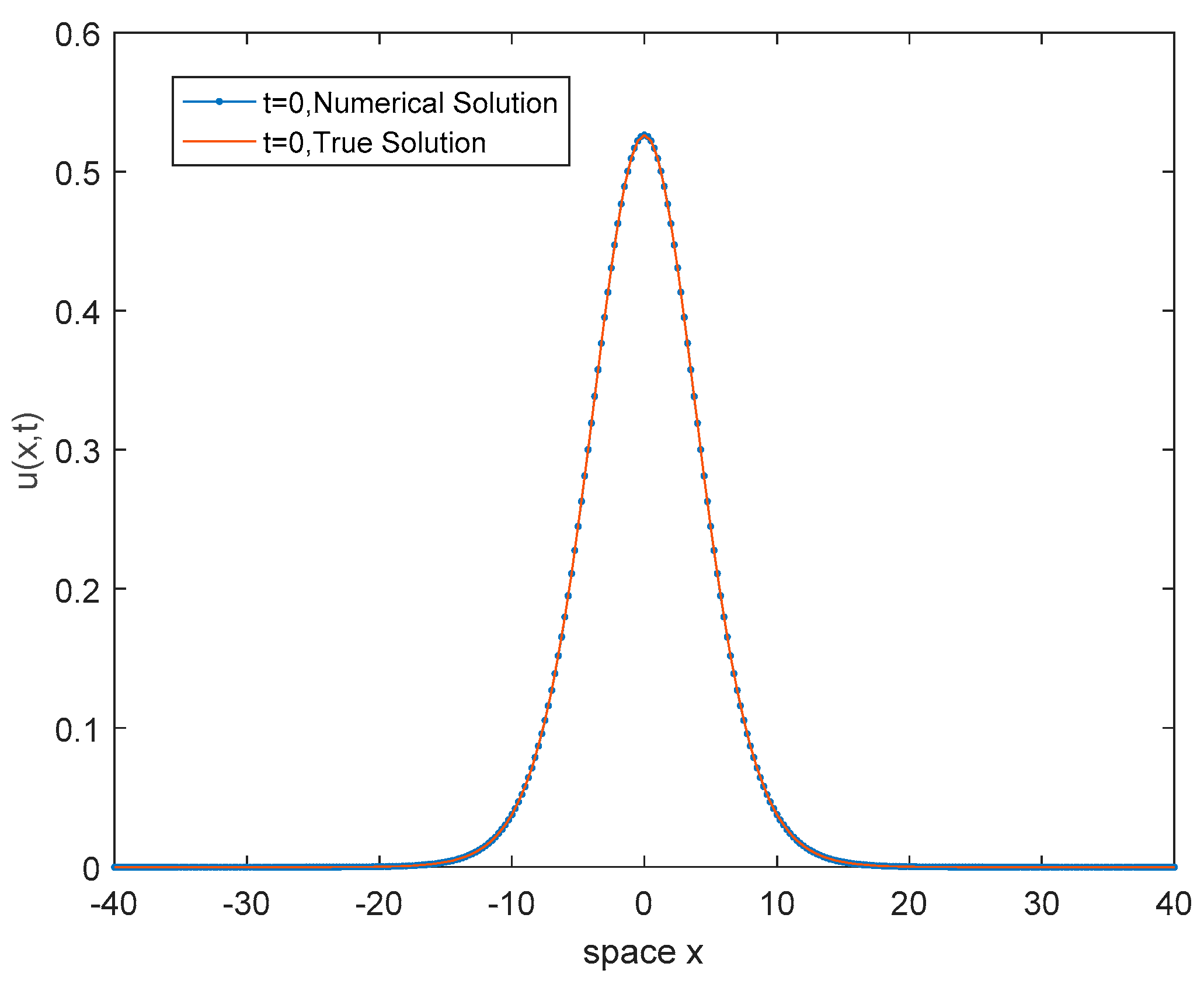
Theorem 6.

The solution of the discrete scheme (18)–(20) is unique.

Proof. 

We assume that $u^n$ and $w^n$ are two different solutions of (18)–(20). Let $S_j^{n+\frac{1}{2}}=w_j^{n+\frac{1}{2}}-u_j^{n+\frac{1}{2}}$. Then, we have

$$\begin{array}{l} \frac{1}{9}\left({\left(S_{j-1}^{n+\frac{1}{2}}\right)}_{\widehat{t}}+7{\left(S_j^{n+\frac{1}{2}}\right)}_{\widehat{t}}+{\left(S_{j+1}^{n+\frac{1}{2}}\right)}_{\widehat{t}}\right)+{\left(S_j^{n+\frac{1}{2}}\right)}_{xx\overline{x}\overline{x}\widehat{t}}+{\left(S_j^{n+\frac{1}{2}}\right)}_{\widehat{x}}+{\left(S_j^{n+\frac{1}{2}}\right)}_{x\overline{x}\widehat{x}}\\ +\frac{1}{3}{\left(w_j^{n+\frac{1}{2}}\right)}_{\widehat{x}}\left(w_{j-1}^{n+\frac{1}{2}}+w_j^{n+\frac{1}{2}}+w_{j+1}^{n+\frac{1}{2}}\right)-\frac{1}{3}{\left(u_j^{n+\frac{1}{2}}\right)}_{\widehat{x}}\left(u_{j-1}^{n+\frac{1}{2}}+u_j^{n+\frac{1}{2}}+u_{j+1}^{n+\frac{1}{2}}\right)=0\end{array}$$

(42)

By computing the inner product of (42) with $2S^{n+\frac{1}{2}}\left(i.e.S^{n+1}+S^n\right)$, we obtain

$$\begin{array}{l} \frac{7}{9\tau }{\Vert S^{n+1}\Vert }^2+\frac{2h}{9\tau }{\displaystyle \sum _{j=1}^{J-1}{S}_j^{n+1}{S}_{j+1}^{n+1}}-\frac{7}{9\tau }{\Vert S^n\Vert }^2-\frac{2h}{9\tau }{\displaystyle \sum _{j=1}^{J-1}{S}_j^n{S}_{j+1}^n}\\ +\frac{1}{\tau }\left({\Vert S_{xx}^{n+1}\Vert }^2-{\Vert S_{xx}^n\Vert }^2\right)+\left(\phi (w)-\phi (u),2e^{n+\frac{1}{2}}\right)=0\end{array}$$

(43)

Let $Z^n=\frac{7}{9}{\Vert S^n\Vert }^2+\frac{2h}{9}{\displaystyle \sum _{j=1}^{J-1}{S}_j^n{S}_{j+1}^n}+{\Vert S_{xx}^n\Vert }^2+{\Vert S_x^n\Vert }^2$; we know that $Z^0=0$. From (43) we obtain

$$Z^{n+1}-Z^n\le C\tau \left({\Vert S^{n+1}\Vert }^2+{\Vert S^n\Vert }^2+{\Vert S_{xx}^{n+1}\Vert }^2+{\Vert S_{xx}^n\Vert }^2+{\Vert S_{\widehat{x}}^{n+1}\Vert }^2+{\Vert S_{\widehat{x}}^n\Vert }^2\right)$$

(44)

Similarly, while $1-2C\tau >0$, we have

$$Z^{n+1}\le \left(1+\beta \tau \right)Z^n\le \cdots \le {\left(1+\beta \tau \right)}^{n+1}{Z}^0=0$$

(45)

Hence, we have ${\Vert S^n\Vert }^2=0$, where $\beta =\frac{4C}{1-2C\tau }$. This implies that $u^n=w^n$. The discrete scheme (18)–(20) is thus uniquely solvable. □

7. Results

7.1. Example

We consider the Rosenau-KdV equation

$$u_t+u_{xxxxt}+u_x+u{u}_x+u_{xxx}=0, \left(x,t\right)\in \left[-40,40\right]\times \left[0,10\right]$$

(46)

with initial condition

$$u\left(x,0\right)=\left(\frac{35}{312}\sqrt{313}-\frac{35}{24}\right){\mathrm{sech}}^4\left[\frac{1}{24}\sqrt{2\sqrt{313}-26}x\right],x\in [-40,40]$$

(47)

and boundary conditions

$$u\left(-40, t\right)=u\left(40, t\right)=0, u_x\left(-40, t\right)=u_x\left(40, t\right)=0, t\in [0,10]$$

(48)

The exact solution is given by

$$u(x, t)=\left(\frac{35}{312}\sqrt{313}-\frac{35}{24}\right){\mathrm{sech}}^4\left\{\frac{\sqrt{2\sqrt{313}-26}}{24}\left[x-\left(\frac{1}{2}+\frac{1}{26}\sqrt{313}\right)t\right]\right\}$$

(49)

7.2. Figures, Tables, and Schemes

We discretize the problem (46)–(48) using the numerical scheme (18)–(20).

From Figure 1, Figure 2, Figure 3, Figure 4, Figure 5 and Figure 6, we can see that the numerical solution is consistent with the exact solution.

In

Table 1. The errors at different times with various $h$ and $\tau$.

	$\mathit{h}=\mathit{\tau }=1/4$		$\mathit{h}=\mathit{\tau }=1/8$
	${\Vert {\mathit{e}}^{\mathit{n}}\Vert }_{\infty }$	$\Vert {\mathit{e}}^{\mathit{n}}\Vert$	${\Vert {\mathit{e}}^{\mathit{n}}\Vert }_{\infty }$	$\Vert {\mathit{e}}^{\mathit{n}}\Vert$
$t=2$	$2.31861708\times {10}^{-4}$	$1.23912354\times {10}^{-3}$	$5.80241511\times {10}^{-5}$	$4.38690718\times {10}^{-4}$
$t=4$	$4.68968494\times {10}^{-4}$	$2.46559087\times {10}^{-3}$	$1.17406720\times {10}^{-4}$	$8.73135975\times {10}^{-4}$
$t=6$	$7.06502002\times {10}^{-4}$	$3.66896388\times {10}^{-3}$	$1.77078291\times {10}^{-4}$	$1.30146495\times {10}^{-3}$
$t=8$	$9.33077015\times {10}^{-4}$	$4.84157574\times {10}^{-3}$	$2.34850462\times {10}^{-4}$	$1.72786004\times {10}^{-3}$
$t=10$	$1.14711186\times {10}^{-3}$	$5.97898965\times {10}^{-3}$	$2.91676007\times {10}^{-4}$	$2.16772647\times {10}^{-3}$

, the errors with various $h$ and $\tau$ are given. It is obvious that the errors are reducing with decreasing $h$ and $\tau$. Hence, our discrete scheme is reasonable. $\Vert e^n(h, \tau )\Vert /\Vert e^n(h/2, \tau /2)\Vert$ and ${\Vert e^n(h, \tau )\Vert }_{\infty }/{\Vert e^n(h/2, \tau /2)\Vert }_{\infty }$ are given in

Table 2. The convergence rateswith various $h$ and $\tau$ and various norms.

	$\Vert {\mathit{e}}^{\mathit{n}}(\mathit{h}, \mathit{\tau })\Vert /\Vert {\mathit{e}}^{\mathit{n}}(\mathit{h}/2, \mathit{\tau }/2)\Vert$			${\Vert {\mathit{e}}^{\mathit{n}}(\mathit{h}, \mathit{\tau })\Vert }_{\mathit{\infty }}/{\Vert {\mathit{e}}^{\mathit{n}}(\mathit{h}/2, \mathit{\tau }/2)\Vert }_{\mathit{\infty }}$
	$\tau =\mathit{h}=1/2$	$\tau =\mathit{h}=1/4$	$\tau =\mathit{h}=1/8$	$\tau =\mathit{h}=1/2$	$\tau =\mathit{h}=1/4$	$\tau =\mathit{h}=1/8$
$t=2$	—	2.81334134	2.82459484	—	3.98408169	3.99595175
$t=4$	—	2.81287147	2.82383379	—	3.96857153	3.99439224
$t=6$	—	2.81210118	2.81910310	—	3.98033046	3.98977197
$t=8$	—	2.81112183	2.80206476	—	3.96316463	3.97306867
$t=10$	—	2.81001148	2.75818454	—	3.97437701	3.93282902

, which interprets the convergence rates of the numerical scheme with various $h$ and $\tau$ and various norms. From

Table 3. Discrete $E_n$ values at different times with various $h$ and $\tau$.

	$\mathit{h}=\mathit{\tau }=1/2$	$\mathit{h}=\mathit{\tau }=1/4$	$\mathit{h}=\mathit{\tau }=1/8$
$t=2$	3.08675012	6.17349199	12.34697937
$t=4$	3.08676651	6.17350095	12.34698364
$t=6$	3.08679087	6.17351432	12.34698593
$t=8$	3.08681918	6.17352996	12.34696462
$t=10$	3.08684844	6.17354622	12.34685552

, we can see that the discrete $E_n$ is conservative. This property is consistent with the original equation. The numerical experiment shows that our discrete scheme is efficient.

8. Conclusions

In this paper, a second-order implicit nonlinear discrete scheme for the Rosenau-KdV equation is proposed via the multiple integral finite volume method (MIFVM). The discrete scheme possesses the conservative property of the original equation. The solvability, uniqueness, convergence, and unconditional stability of the scheme were demonstrated in detail. Numerical experiments verified that the discrete scheme given by MIFVM is effective.

References

1. Yokus, A.; Bulut, H. Numerical simulation of KdV equation by finite difference method. Indian J. Phys. 2018, 92, 1571–1575. [Google Scholar] [CrossRef]
2. Başhan, A. A novel approach via mixed Crank–Nicolson scheme and differential quadrature method for numerical solutions of solitons of mKdV equation. Pramana-J. Phys. 2019, 92, 84. [Google Scholar] [CrossRef]
3. Başhan, A.; Yağmurlu, N.M.; Uçar, Y.; Esen, A. A new perspective for the numerical solutions of the cmKdV equation via modified cubic B-spline differential quadrature method. Int. J. Mod. Phys. C 2018, 29, 1850043. [Google Scholar] [CrossRef]
4. Kong, D.; Xu, Y.; Zheng, Z. Numerical method for generalized time fractional KdV-type equation. Numer. Methods Partial. Differ. Equ. 2019, 36, 906–936. [Google Scholar] [CrossRef]
5. Cairone, F.; Anandan, P.; Bucolo, M. Nonlinear systems synchronization for modeling two-phase microfluidics flows. Nonlinear Dyn. 2017, 92, 75–84. [Google Scholar] [CrossRef]
6. Wazwaz, A.-M. A new integrable equation that combines the KdV equation with the negative-order KdV equation. Math. Methods Appl. Sci. 2018, 41, 80–87. [Google Scholar] [CrossRef]
7. Wazwaz, A.-M. Negative-order KdV equations in (3 + 1) dimensions by using the KdV recursion operator. Waves Random Complex Media 2017, 27, 768–778. [Google Scholar] [CrossRef]
8. Rosenau, P. A Quasi-Continuous Description of a Nonlinear Transmission Line. Phys. Scr. 1986, 34, 827–829. [Google Scholar] [CrossRef]
9. Rosenau, P. Dynamics of Dense Discrete Systems: High Order Effects. Prog. Theor. Phys. 1988, 79, 1028–1042. [Google Scholar] [CrossRef] [Green Version]
10. Park, M.A. On the Rosenau equation. Matemática Aplic. Comput. 1990, 9, 145–152. [Google Scholar]
11. Erbay, H.; Erbay, S.; Erkip, A. Numerical computation of solitary wave solutions of the Rosenau equation. Wave Motion 2020, 98, 102618. [Google Scholar] [CrossRef]
12. Atouani, N.; Ouali, Y.; Omrani, K. Mixed finite element methods for the Rosenau equation. J. Appl. Math. Comput. 2018, 57, 393–420. [Google Scholar] [CrossRef]
13. Michihisa, H. New asymptotic estimates of solutions for generalized Rosenau equations. Math. Methods Appl. Sci. 2019, 42, 4516–4542. [Google Scholar] [CrossRef]
14. Shi, D.; Jia, X. Superconvergence analysis of the mixed finite element method for the Rosenau equation. J. Math. Anal. Appl. 2020, 481, 123485. [Google Scholar] [CrossRef]
15. Safdari-Vaighani, A.; Larsson, E.; Heryudono, A. Radial Basis Function Methods for the Rosenau Equation and Other Higher Order PDEs. J. Sci. Comput. 2018, 75, 1555–1580. [Google Scholar] [CrossRef] [Green Version]
16. Wang, Y.; Feng, G. Large-time behavior of solutions to the Rosenau equation with damped term. Math. Methods Appl. Sci. 2017, 40, 1986–2004. [Google Scholar] [CrossRef]
17. Wang, X.; Dai, W. A conservative fourth-order stable finite difference scheme for the generalized Rosenau–KdV equation in both 1D and 2D. J. Comput. Appl. Math. 2019, 355, 310–331. [Google Scholar] [CrossRef]
18. Luo, Y.; Xu, Y.; Feng, M. Conservative Difference Scheme for Generalized Rosenau-KdV Equation. Adv. Math. Phys. 2014, 2014, 986098. [Google Scholar] [CrossRef] [Green Version]
19. Hussain, M.; Haq, S. Numerical simulation of solitary waves of Rosenau–KdV equation by Crank–Nicolson meshless spectral interpolation method. Eur. Phys. J. Plus 2020, 135, 98. [Google Scholar] [CrossRef]
20. Kutluay, S.; Karta, M.; Yağmurlu, N.M. Operator time-splitting techniques combined with quintic B-spline collocation method for the generalized Rosenau–KdV equation. Numer. Methods Partial. Differ. Equ. 2019, 35, 2221–2235. [Google Scholar] [CrossRef]
21. Browder, F.E. Existence and uniqueness theorems for solutions of nonlinear boundary value problems. In Proceedings of the Sum of Squares: Theory and Applications; American Mathematical Society: Providence, RI, USA, 1965; Volume 17, pp. 24–49. [Google Scholar]
22. Zhou, Y.L. Applications of Discrete Functional Analysis to the Finite Difference Method, 1st ed.; International Academic Publishers: Beijing, China, 1991; pp. 3–20. [Google Scholar]
Figure 1. Numerical solution and exact solution with h = τ = 1 / 4 , t = 0 .
Mathematics 09 01183 g001
Figure 2. Numerical solution and exact solution with h = τ = 1 / 4 , t = 5 .
Mathematics 09 01183 g002
Figure 3. Numerical solution and exact solution with h = τ = 1 / 4 , t = 10 .
Mathematics 09 01183 g003
Figure 4. Numerical solution and exact solution with   h = τ = 1 / 8   , t = 0 .
Mathematics 09 01183 g004
Figure 5. Numerical solution and exact solution with   h = τ = 1 / 8   , t = 5 .
Mathematics 09 01183 g005
Figure 6. Numerical solution and exact solution with   h = τ = 1 / 8   , t = 10 .
Mathematics 09 01183 g006