Residue Sum Formula for Pricing Options under the Variance Gamma Model

Abstract

We present and prove a triple sum series formula for the European call option price in a market model where the underlying asset price is driven by a Variance Gamma process. In order to obtain this formula, we present some concepts and properties of multidimensional complex analysis, with particular emphasis on the multidimensional Jordan Lemma and the application of residue calculus to a Mellin–Barnes integral representation in ${\mathbb{C}}^3$, for the call option price. Moreover, we derive triple sum series formulas for some of the Greeks associated to the call option and we discuss the numerical accuracy and convergence of the main pricing formula.

1. Introduction

The pricing of financial derivatives, such as options, is one of the pivotal tasks of mathematical finance, yet it can be an arduous task to develop a model that is consistent with the empirical evidence, soluble, and where its numerical estimation is neither erroneous nor time consuming. One of the first attempts to solve this quandary was the Gaussian model that was first introduced by Fischer Black and Myron Scholes in [1] and later expanded by Robert Merton in [2], aptly named the Black–Scholes model, where the stochastic process driving the underlying asset price is modeled by a geometric Brownian motion. Its simplicity and the admission of a close formula for the option price are the main reasons why, to this day, it remains the most frequently used model by market practitioners. Still, the model fails to account for sudden price drops or increases that can be expressed as discontinuous price jumps; moreover, it assumes the volatility to remain constant for changes in relation to the strike price and time to maturity, contrary to the evidence derived from empirical data and, furthermore, the distributions of asset returns have been shown to be negatively skewed and exhibit fat-tails that are not captured by the symmetric Gaussian model.

The Black–Scholes model has been generalized in many ways. Let us mention two of the most important classes of models used in these generalizations: stochastic volatility models and jump models (see [3]). The model that we consider in this paper is a particular jump model, which assumes that the underlying asset price dynamics are described by a Lévy Process, namely the Variance Gamma process, which was first proposed by Dilip Madan and Eugene Seneta in [4]. The descriptive power of models that are based on Lévy processes for accurately portraying financial markets (not displaying the aforementioned problems that are present in the Black–Scholes model) has been known since the works of Benoît Mandelbrot [5] and Eugene Fama [3], and they have been gaining traction in recent decades with the advent of technology and computer development. Yet, the Black–Scholes model remains mostly ubiquitous. The main reason for this state of affairs is that pricing models that are based on Lévy processes admit, at best, a closed pricing formula for some particular cases, but, in general, prices must be computed by numerical simulation.

Several authors have studied the problem of option pricing under the Variance Gamma model. Let us highlight some important contributions. In [6], the authors obtain a closed form formula for the price of a European call option. This formula involves the evaluation of a modified Bessel function and a degenerate Hypergeometric function. A numerical method for option pricing based on Fourier Transform and Fast Fourier Transform was proposed in [7] and a method based on the Fourier-cosine series was proposed in [8]. An alternative numerical approach to the problem is based on the development of finite difference schemes for obtaining the solution of the partial integro-differential equation (PIDE) for the option pricing function (see, for instance, [9]). A multinomial method for option pricing of European and American options under the Variance Gamma model was also proposed and discussed in [10].

In recent years, a different approach has been undertaken directed at $\alpha$-stable Lévy processes (see [11]), which include: the discovery of the conditions for guaranteeing the existence of a martingale measure, which was carried out by Peter Carr and Liuren Wu in [12]; the representation of the Green function (the fundamental solution to the space–time fractional diffusion equation) by a Mellin–Barnes integral of a Gamma fraction, which was done by Rudolf Gorenflo and Francesco Mainardi, among others (see [13,14,15,16] for more details); and, the discovery that, under certain conditions, Residue Calculus can be applied to a Mellin–Barnes integral of a Gamma fraction, converting it into a multiple sum series, by Mikael Passare, August Tsikh, and Oleg Zhadanov in [17,18,19]. Let us briefly describe why the Mellin–Barnes integral is important when studying the space–time fractional diffusion equation (which generalizes the standard diffusion equation by replacing the usual derivatives with fractional derivatives). The fundamental solution or Green function of the fractional diffusion equation can be represented as a spatial density probability function that is time dependent. After applying the Mellin transform to this Green function, one obtains a Mellin–Barnes integral of Gamma functions in the complex plane. This Mellin–Barnes integral can be evaluated using the residues theorem and represented by a convergent series (for more details, see [13]). Finally, Jean-Phillipe Aguilar, Cyril Coste, and Jan Korbel used the Green function to express the price of a European option as a Mellin–Barnes integral in their works [20,21,22], and they were able to arrive at a double series representation for the European call option price by applying the previously mentioned results that were developed by Passare et al.

The main novelty and major contribution of the present study is that we obtain and prove a Mellin–Barnes integral representation and the associated triple residue sum formulas for European option prices and Greek functions, by using three-dimensional complex analysis in ${\mathbb{C}}^3$ and considering the Variance Gamma model for the dynamics of the underlying risky asset. We also confirmed the viability and accuracy of the formula obtained by using numerical tests on real option data. Note that, in [20,21,22], a similar approach was applied to the time-fractional diffusion and the particular case of the finite moment Lévy stable model. However, in these papers, only two-dimensional complex analysis in ${\mathbb{C}}^2$ was required and a double residue sum formula was obtained. Let us also note that, in [4], the authors introduce the Variance Gamma model for option pricing, but they use a very different approach for the calculation of the option price: the traditional risk neutral valuation formula and numerical integration techniques, when considering the probability density function of the Variance Gamma distribution.

The organization of the paper follows below. In Section 2, we will introduce preliminary concepts, such as the multidimensional Residue Theory and Mellin–Barnes integral, and discuss some of their properties. In Section 3, we present the option pricing problem and prove the representation of the triple Mellin–Barnes Integral for the option price. In Section 4, we present the main results of the paper. By applying residue calculus, we derive the triple series representation for the European call option price under the Variance Gamma model and the subsequent Greek functions. In Section 5, taking advantage of the data presented in [23], we test the accuracy of the Variance Gamma formula and its Greeks. The last section is dedicated to some concluding remarks.

2. Preliminary Theory

2.1. Multidimensional Residue Calculus

We start by enumerating, without proving, some of the definitions and results of multidimensional complex analysis. A more in-depth theoretical introduction to multidimensional complex analysis can be found in the textbooks [24,25].

Definition 1

(Grothendieck Residue). Let h and $f_i$, for any index $i\in \{1,\dots ,n\}$, be functions in ${\mathbb{C}}^n$, where h is holomorphic. Consider the meromorphic differential n-form

$$\begin{array}{c}\hfill \omega =\frac{h\left(z\right)dz}{f_1\left(z\right)\dots f_n\left(z\right)},dz=d{z}_1\wedge \dots \wedge d{z}_n,\end{array}$$

(1)

which has the singularities $D_j=\{z\in \mathbb{C}:f_j\left(z\right)=0\}$, such that the intersection ${\bigcap }_{j=1}^n{D}_j$ is discrete. The Grothendieck residue on a singularity $a\in {\bigcap }_{j=1}^n{D}_j$ is defined as

$$\begin{array}{c}\hfill {\mathrm{Res}}_a\omega =\frac{1}{{\left(2\pi i\right)}^n}{\int }_{C_a}\omega ,\end{array}$$

(2)

where $C_a=\{z\in U_a:|f_j\left(z\right)|=ϵ,j=1,\dots ,n\}$ is a cycle in a small neighborhood $U_a$ of the singularity a with the orientation $d(arg{f}_1)\wedge \dots \wedge d(arg{f}_n)\ge 0$.

Before proceeding we will formalize the concept of a multidimensional polyhedron in ${\mathbb{C}}^n$. The two following definitions will underpin most of the theorems from Section 2 and Section 3.

Definition 2

(Polyhedron). Consider a proper (the inverse images of a compact set are compact) holomorphic map $g:{\mathbb{C}}^n\to G$ where $G=G_1\times \dots \times G_n$ is a domain (connected open subset of a finite-dimensional vector space) where, for each $j=1,\dots ,n$, $G_j\subset \mathbb{C}$ is a domain with piecewise smooth boundary. We define a polyhedron Π as the inverse image

$$\begin{array}{c}\hfill \mathrm{\Pi }:=g^{-1}\left(G\right),\end{array}$$

(3)

and for a multi-index $K=\{k_1,\dots ,k_p\}\subset \{1,\dots ,n\}$ we define the polyhedron’s faces as

$$\begin{array}{c}\hfill {\sigma }_K:=\{z:g_k\left(z\right)\in \partial G_{k}fork\in K,g_j\left(z\right)\in G_{j}forj\in K^C\}.\end{array}$$

(4)

Definition 3

(Compatible divisors). Consider the polyhedron Π and the family of divisors ${\left\{D_i\right\}}_{i\in \{1,\dots ,n\}}$, they are said to be compatible if for any $i\in \{1,\dots ,n\}$ we get

$$\begin{array}{c}\hfill {\sigma }_i\cap D_i=\varnothing .\end{array}$$

(5)

Analogously to the one dimensional integral on the real axis, we may want to compute an integral ${\int }_{\sigma }\omega$ where $\omega$ is the meromorphic form (1) and $\sigma$ is the boundary of a polyhedron $\mathrm{\Pi }$. For an unbounded polyhedron we need the integrand to vanish as it goes to infinity. To achieve this goal let us introduce the auxiliary functions

$$\begin{array}{c}\hfill {\rho }_j=\frac{|f_j{|}^2}{{∥f∥}^2},\mathrm{for}\mathrm{any}j\in \{1,\dots ,n\},\end{array}$$

(6)

where ${∥f∥}^2=|f_1{|}^2+\dots +{\left|f_n\right|}^2$. Using the functions (6) we define the differential $(n,p-1)$-forms as

$$\begin{array}{c}\hfill {\xi }_J=\sum _{j\in J}{(-1)}^{(j,J)-1}{\rho }_j\overline{\partial }{\rho }_J\left[j\right]\wedge \omega ,\end{array}$$

(7)

where $J=\{j_1,\dots ,j_s\}\subset \{1,\dots ,n\}$, for $1<s\le n$, is a multi-index, $(j,J)$ is the position of j in set J and $\overline{\partial }{\rho }_J\left[j\right]=\overline{\partial }{\rho }_{j_1}\wedge \dots \left[j\right]\dots \wedge {\overline{\partial }}_{j_s}$. We now define the multidimensional condition analogous to ${lim}_{R\to \infty }{\int }_{S_R}f\left(z\right)dz=0$.

Definition 4

(Jordan condition). Consider the sphere $S_R=\{z\in \sigma :∥z∥=R\}$, where $\sigma ={\sigma }_{12\dots n}$ is the boundary of the polyhedron Π. A differential form ${\xi }_J$ satisfies the Jordan condition on face ${\sigma }_{J^o}$, with $J^o=\{1,\dots ,n\}\backslash J$, if exists a sequence of positive real numbers $R_k$ that goes to infinity, such that

$$\begin{array}{c}\hfill \underset{k\to \infty }{lim}{\int }_{S_{R_k}\cap {\sigma }_{J^o}}{\xi }_J=0.\end{array}$$

(8)

Note that, for $n=1$, there exists only one form $\xi =\omega$ and thus the condition (8) corresponds to the unidimensional condition ${lim}_{z\to \infty }{\int }_{S_R}f\left(z\right)dz=0$. For the multidimensional case, consider the set $N=\{z\in {\mathbb{C}}^n:∥f\left(z\right)∥=0\}={\bigcap }_{i=1}^n{D}_i$. Thus, we have the following theorem, which allows us to compute the integral of the meromorphic form (1) on the boundary of the polyhedron as a sum of residues, and it is the main theoretical tool used in the proof of Theorem 2.

Theorem 1

(The Jordan Lemma). Let ω be a meromorphic form with the polar divisors ${\left\{D_i\right\}}_{i\in \{1,\dots ,n\}}$ compatible with polyhedron Π. If, for every multi-index J, the differential form ${\xi }_J$ satisfies the Jordan condition on ${\sigma }_{J^o}$, then we get

$$\begin{array}{c}\hfill {\int }_{\sigma }\omega ={\left(2\pi i\right)}^n\sum _{a\in N\cap \mathrm{\Pi }}{\mathrm{Res}}_a\omega \end{array}$$

(9)

The Jordan’s Lemma proof can be found in [17].

2.2. One-Dimensional Mellin–Barnes Integral

We will start by presenting, without proof, some basic concepts and properties for the one-dimensional Mellin–Barnes integral. For a more in depth look at Fourier, Laplace, and Mellin Transforms, as well as their corresponding properties, we recommend the book [26].

Definition 5

(Mellin–Barnes Integral). The Mellin–Barnes Integral is given by a ratio of products of Gamma functions of linear arguments

$$\mathrm{\Phi }\left(t\right):=\frac{1}{2\pi i}{\int }_{\gamma -i\infty }^{\gamma +i\infty }\frac{{\prod }_{j=1}^m\mathrm{\Gamma }(a_{j}z+b_j)}{{\prod }_{k=1}^p\mathrm{\Gamma }(c_{k}z+d_k)}{t}^{-z}dz,$$

(10)

where its characteristic quantity, Δ, is defined by

$$\Delta =\sum _{j=1}^m{a}_j-\sum _{k=1}^p{c}_k$$

(11)

Before proceeding, let us state the Stirling’s approximation of the gamma function (see [27])

$$\begin{array}{c}\hfill \mathrm{\Gamma }\left(z\right)=\sqrt{2\pi }{z}^{z-1/2}{e}^{-z}O\left(1+\frac{1}{z}\right)\underset{\left|z\right|\to \infty }{\to }\sqrt{2\pi }{z}^{z-1/2}{e}^{-z}.\end{array}$$

(12)

Equipped with this expression, one can easily see how $\Delta$ governs the behavior of the ratio of Gammas as $\left|z\right|\to \infty$, and, therefore, which residues, of the singularities to the left or right of the $\Im \left(z\right)=0$ strip, one will sum to compute the integral (10):

$$\begin{array}{c}\hfill \mathrm{\Phi }\left(t\right)=\left\{\begin{array}{cc}{\displaystyle \sum _{\Re \left(s_n\right)<\gamma }}{\mathrm{Res}}_{s_n}\left(\frac{{\prod }_{j=1}^m\mathrm{\Gamma }(a_{j}z+b_j)}{{\prod }_{k=1}^p\mathrm{\Gamma }(c_{k}z+d_k)}\right)t^{-s_n}\hfill & \mathrm{if}\Delta >0,\hfill \\ -{\displaystyle \sum _{\Re \left(s_n\right)>\gamma }}{\mathrm{Res}}_{s_n}\left(\frac{{\prod }_{j=1}^m\mathrm{\Gamma }(a_{j}z+b_j)}{{\prod }_{k=1}^p\mathrm{\Gamma }(c_{k}z+d_k)}\right)t^{-s_n}\hfill & \mathrm{if}\Delta <0.\hfill \end{array}\right.\end{array}$$

(13)

For example, one can express an exponential term $e^x$ as the Mellin–Barnes integral

$$\begin{array}{c}\hfill e^x=\sum _{n=0}^{\infty }\frac{x^n}{n!}=\underset{\gamma -i\infty }{\overset{\gamma +i\infty }{\int }}{(-1)}^{-t}\mathrm{\Gamma }\left(t\right)x^{-t}\frac{dt}{2\pi i},\end{array}$$

(14)

where $\gamma >0$.

2.3. Three-Dimensional Mellin–Barnes Integral

In this subsection, similarly to what we did previously for the unidimensional case, we will present the triple Mellin–Barnes integral and deduce its formula as a sum of residues, which will be crucial when proving the main result of this paper. In order to achieve this, let us first consider its integral form

$$\begin{array}{c}\hfill \mathrm{\Phi }\left(t\right)=\frac{1}{{\left(2\pi i\right)}^3}\underset{\gamma +i{\mathbb{R}}^3}{\int }\frac{{\displaystyle \prod _{j=1}^m}\mathrm{\Gamma }(a_{j1}{z}_1+a_{j2}{z}_2+a_{j3}{z}_3+b_j)}{{\displaystyle \prod _{k=1}^p}\mathrm{\Gamma }(c_{k1}{z}_1+c_{k2}{z}_2+c_{k3}{z}_3+d_j)}{t}^{-z_1}{t}^{-z_2}{t}^{-z_3}d{z}_1\wedge d{z}_2\wedge d{z}_3.\end{array}$$

(15)

Henceforth, for brevity, we will denote the three-form integrand of (15) by $\omega$. Its zeroes will be the complex planes $L_j^{\nu }=\{(z_1,z_2,z_3)\in {\mathbb{C}}^3:a_{j1}{z}_1+a_{j2}{z}_2+a_{j3}{z}_3+b_j=-\nu \}$, for any $\nu \in \mathbb{N}$ and $j\in \{1,\dots ,m\}$, which represent each singularity given by the gamma functions present in the numerator of the form $\omega$. We will also denote the vectors ${\underline{a}}_j:=\left[\begin{array}{c}{a}_{j1}\\ a_{j2}\\ a_{j3}\end{array}\right]$, ${\underline{c}}_k:=\left[\begin{array}{c}{a}_{k1}\\ a_{k2}\\ a_{k3}\end{array}\right]$ and, most importantly, define the characteristic vector as

$$\begin{array}{c}\hfill \Delta =\sum _{j=1}^m{\underline{a}}_j-\sum _{k=1}^p{\underline{c}}_k.\end{array}$$

(16)

Suppose that $\Delta$ is a non-zero vector. In this case, we can define the plane $P_{\Delta }$ where its real part intersects the point $\gamma$ and has $\Delta$ as its normal vector, i.e., $P_{\Delta }:=\{z\in {\mathbb{C}}^3:\Re \left(⟨\Delta ,z⟩\right)=\Re \left(⟨\Delta ,\gamma ⟩\right)\}$, and thereupon we can define the admissible-polyhedra, ${\mathrm{\Pi }}_{\Delta }$, as the real volume “below” $P_{\Delta }$, i.e., ${\mathrm{\Pi }}_{\Delta }:=\{z\in {\mathbb{C}}^3:\Re \left(⟨\Delta ,z⟩\right))\le \Re \left(⟨\Delta ,\gamma ⟩\right)\}$.

Taking all of these previous demarcations into account, we can construct an admissible polyhedron $\mathrm{\Pi }\subset {\mathrm{\Pi }}_{\Delta }$, which will be uniquely defined by the linear function $g:{\mathbb{C}}^3\to G$, where $\mathrm{\Pi }=g^{-1}\left(G\right)$ and

$$\begin{array}{c}\hfill g\left(z\right)=\left[\begin{array}{c}{n}_1\\ n_2\\ n_3\end{array}\right]\left(\Re \left(z\right)-\gamma \right)+i\Im \left(z\right),\end{array}$$

(17)

with the image $G=\{z\in C^3:\Re \left(z_1\right)\ge 0,\Re \left(z_2\right)\ge 0,\Re \left(z_3\right)\ge 0\}$, i.e the first octant. From (17), we can ascertain that its only vertex is ${\sigma }_{1,2,3}=\gamma$ and that $n_1$, $n_2$, and $n_3$ are the normal vectors of the faces ${\sigma }_1$, ${\sigma }_2$, and ${\sigma }_3$ of the polyhedron:

$$\begin{array}{cc}\hfill & {\sigma }_1=\{z\in {\mathbb{C}}^3:\Re \left(⟨n_1,z⟩\right)=\Re \left(⟨n_1,z⟩\right),\Re \left(⟨n_2,z⟩\right)\ge \Re \left(⟨n_2,z⟩\right),\Re \left(⟨n_3,z⟩\right)\ge \Re \left(⟨n_3,z⟩\right)\},\hfill \end{array}$$

(18)

$$\begin{array}{cc}\hfill & {\sigma }_2=\{z\in {\mathbb{C}}^3:\Re \left(⟨n_1,z⟩\right)\ge \Re \left(⟨n_1,z⟩\right),\Re \left(⟨n_2,z⟩\right)=\Re \left(⟨n_2,z⟩\right),\Re \left(⟨n_3,z⟩\right)\ge \Re \left(⟨n_3,z⟩\right)\},\hfill \end{array}$$

(19)

$$\begin{array}{cc}\hfill & {\sigma }_3=\{z\in {\mathbb{C}}^3:\Re \left(⟨n_1,z⟩\right)\ge \Re \left(⟨n_1,z⟩\right),\Re \left(⟨n_2,z⟩\right)\ge \Re \left(⟨n_2,z⟩\right),\Re \left(⟨n_3,z⟩\right)=\Re \left(⟨n_3,z⟩\right)\}.\hfill \end{array}$$

(20)

If the polyhedron was providently constructed, then we can balkanize the singularities, $L_j^{\nu }$, into three distinct sets, such that they are compatible with the polyhedron, i.e.:

$$\begin{array}{c}\hfill D_1=\bigcup _{\begin{array}{c}j\in \{1,\dots ,m\}\\ \nu \in \mathbb{N}\\ L_j^{\nu }\cap {\sigma }_1=\varnothing \end{array}}{L}_j^{\nu },D_2=\bigcup _{\begin{array}{c}j\in \{1,\dots ,m\}\\ \nu \in \mathbb{N}\\ L_j^{\nu }\cap {\sigma }_2=\varnothing \end{array}}{L}_j^{\nu },D_3=\bigcup _{\begin{array}{c}j\in \{1,\dots ,m\}\\ \nu \in \mathbb{N}\\ L_j^{\nu }\cap {\sigma }_3=\varnothing \end{array}}{L}_j^{\nu }.\end{array}$$

(21)

Theorem 2

(Residue formula for the Triple Mellin–Barnes integral). Let ω be the three-form integrand of (15) with the characteristic vector $\Delta \ne 0$ and divisors $D_1$, $D_2$, and $D_3$, as defined in (21), being compatible with the admissible polyhedron $\mathrm{\Pi }\subset {\mathrm{\Pi }}_{\Delta }$. Subsequently, the sum formula holds:

$$\begin{array}{c}\hfill \frac{1}{{\left(2\pi i\right)}^3}\underset{\gamma +i{\mathbb{R}}^3}{\int }\omega =\sum _{t\in \mathrm{\Pi }\cap D_1\cap D_2\cap D_3}{\mathrm{Res}}_t\omega ,\end{array}$$

(22)

where the series on the right-hand side converges absolutely for any $\underline{t}\in U$, for U, defined as,

$$U=\{t\in {(\mathbb{C}\backslash 0)}^3:|arg{t}_1|<\pi ,|arg{t}_2|<\pi ,|arg{t}_3|<\pi ,∥argt∥<(\pi /2)\alpha \}$$

(23)

and α is a constant that is given by,

$$\alpha :=\underset{y\in S_1}{min}\left(\sum _{j=1}^m|⟨{\underline{a}}_j,y⟩|-\sum _{j=1}^p\left|⟨{\underline{c}}_j,y⟩\right|\right),$$

(24)

where $S_1=\{y\in {\mathbb{R}}^3:\left|y\right|=1\}$ is the unit sphere in ${\mathbb{R}}^3$.

For a proof of Theorem 2, please see Appendix A.

3. Option Pricing Driven by a Variance Gamma Process

Equipped with the results of the previous section, we will now center our attention on deducing the main result of this paper, the formula for the price of a European call option under the Variance Gamma model. Similar to the derivation presented in [20], we will arrive at this result in two steps. First, we will derive the Mellin–Barnes representation for the aforementioned call option price and, secondly, we will use residue calculus to derive the triple sum series formula.

3.1. Mellin–Barnes Representation for a Call Option

Before introducing the call option price, let us recall that we can define the Variance Gamma process as the difference between two independent gamma processes (see [6]),

$$X_{VG}(\tau ;C,G,M)=G_{\tau }^1-G_{\tau }^2,$$

(25)

where $\tau$ is the time variable, $G_{\tau }^1\sim Gamma(C\tau ,1/M)$ and $G_{\tau }^2\sim Gamma(C\tau ,1/G)$ with parameters $C>0$, $M>0$, and $G>0$. The probability density function of a gamma process $G\sim Gamma(\alpha ,\beta )$ is given by

$$f_{G(\alpha ,\beta )}\left(x\right)=\frac{{\beta }^{\alpha }}{\mathrm{\Gamma }\left(\alpha \right)}{x}^{\alpha -1}{e}^{-\beta x}.$$

(26)

Under these definitions, one can, by direct computation, easily arrive at the characteristic function for the variance gamma process $X_{VG}(\tau ;C,G,M)$,

$${\varphi }_{VG}(u,\tau ;C,G,M)=\mathbb{E}\left[e^{iu{X}_{VG}(\tau ;C,G,M)}\right]={\left[\frac{MG}{MG+iu(M-G)+u^2}\right]}^{-C\tau },$$

(27)

where $u\in \mathbb{R}$ is the main variable of the characteristic function and $\tau$ is the time variable.

Let us now briefly discuss the standard problem of option pricing. For more details about this problem, we refer to [28]. Consider that we have an underlying risky asset with price process denoted by the stochastic process ${\left\{S_t\right\}}_{t\in [0,T]}$, where T denotes the maturity of the European option that we want to evaluate. In our market model, we assume that the continuously compounded risk-free interest rate is denoted by the parameter r and q represents the dividend yield. In the standard Black–Scholes model, it is well known that the market is arbitrage-free and complete. Moreover, we know from the fundamental theorems of asset pricing that an equivalent martingale measure or risk-neutral measure $\mathbb{Q}$ exists if and only if the market is arbitrage-free, and the measure $\mathbb{Q}$ is unique if and only if the market is complete. Therefore, under the standard Black–Scholes model, the equivalent martingale measure $\mathbb{Q}$ exists and it is unique. The measure $\mathbb{Q}$ is equivalent to the real (physical) probability measure $\mathbb{P}$ and the process ${\left\{S_t{e}^{-(r-q)t}\right\}}_{t\in [0,T]}$ is a martingale under $\mathbb{Q}$. The underlying risky asset price at time T, under the measure $\mathbb{Q}$, is given by

$$S_T=S_t{e}^{\left(r-q-\frac{{\sigma }^2}{2}\right)\tau +B_{\tau }^{\mathbb{Q}}},$$

(28)

where $\tau =T-t$ and $B_{\tau }^{\mathbb{Q}}$ is a standard Brownian motion under measure $\mathbb{Q}$.

When considering Lévy Processes (like the Variance Gamma process), the market is, in general, incomplete and many equivalent martingale measures exist. Using the mean correcting martingale measure is one standard way to choose just one equivalent martingale measure. Under this particular measure, in the market model that is driven by the Variance Gamma process, we have that the risky asset price at time T is given by

$$S_T=S_t{e}^{(r-q)\tau -\mu \tau +X_{VG}(\tau ;C,G,M)},$$

(29)

where $\mu :=log\left({\varphi }_{VG}(-i,1;C,G,M)\right)$ is the mean correcting parameter. For more details on the mean correcting martingale measure and the mean correcting parameter, see Chapter 6 of [23]. Let us recall that a European call option with maturity T and strike price $K>0$ is a contract that gives the buyer of the contract the right, but not the obligation, to buy the underlying risky asset at time T by the price K. The payoff of the call option is given by ${\left(S_T-K\right)}^{+}$. Using the well-known risk-neutral valuation formula for option pricing, we can write the price at time t of a European call option with maturity T and strike price $K>0$ as the discounted expected value

$$C(S,K,r,q,\tau )=e^{-r\tau }{\mathbb{E}}^{\mathbb{Q}}\left[{(S{e}^{(r-q)\tau -\mu \tau +X_{VG}(\tau ;C,G,M)}-K)}^{+}\right],$$

(30)

where the variables are the underlying risky asset price at time t (denoted by $S=S_t$), the strike price of the option K, the risk-free interest rate r, the dividend yield q, and the time until maturity $\tau =T-t$.

Using the notation introduced in the previous paragraphs, we can now state and derive the Mellin–Barnes integral representation in ${\mathbb{C}}^3$ for the European call option price under the Variance Gamma model.

Proposition 1

(The Mellin–Barnes representation for a Call Option under Variance Gamma). Let us denote $[log]:=log\frac{S}{K}+(r-q)\tau -\mu \tau$, where $\mu =log\left({\varphi }_{VG}(-i,1;C,G,M)\right)$. Consider the polyhedra $P_1,P_2\subset {\mathbb{C}}^3$, which is defined by

$$\begin{array}{cc}\hfill P_1& :=\{\underline{z}\in {\mathbb{C}}^3:0<\Re \left(z_1\right)<1,0<\Re \left(z_2\right),0<\Re \left(z_3\right)<C\tau ,\hfill \end{array}$$

$$\begin{array}{cc}\hfill & \Re \left(z_1\right)+\Re \left(z_2\right)+\Re \left(z_3\right)>1+2C\tau \},\hfill \end{array}$$

(31)

$$\begin{array}{cc}\hfill P_2& :=\{\underline{z}\in {\mathbb{C}}^3:0<\Re \left(z_1\right)<1,0<\Re \left(z_2\right)<C\tau ,0<\Re \left(z_3\right)<C\tau \}.\hfill \end{array}$$

(32)

Subsequently, the price of a European call option that is driven by the Variance Gamma process is given by the formula

$$\begin{array}{cc}\hfill C_{VG}(S,K,r,q,\tau )& =\frac{K{\left(GM\right)}^{C\tau }{e}^{-r\tau }}{\mathrm{\Gamma }{\left(C\tau \right)}^2}(I_{VG}^1(S,K,r,q,\tau )+{𝕝}_{[log]>0}{I}_{VG}^2(S,K,r,q,\tau ))\hfill \end{array}$$

(33)

where, for any ${\underline{c}}_1\in P_1$ and ${\underline{c}}_2,\in P_2$, we define $I_{VG}^1$ and $I_{VG}^2$ by

$$\begin{array}{cc}\hfill I_{VG}^1(S,K,r,q,\tau ):=& \underset{{\underline{c}}_1+i{\mathbb{R}}^3}{\int }{(-1)}^{-t}\frac{\mathrm{\Gamma }\left(t\right)\mathrm{\Gamma }\left(t_x\right)\mathrm{\Gamma }\left(t_y\right)\mathrm{\Gamma }(1-t)\mathrm{\Gamma }(C\tau -t_y)\mathrm{\Gamma }(-1-2C\tau +t+t_x+t_y)}{\mathrm{\Gamma }(1-C\tau +t_x)}\hfill \end{array}$$

$$\begin{array}{cc}\hfill & \times M^{-t_x}{G}^{-t_y}{(-[log])}^{1+2C\tau -t-t_x-t_y}\frac{dt}{2\pi i}\wedge \frac{d{t}_x}{2\pi i}\wedge \frac{d{t}_y}{2\pi i},\hfill \\ \hfill I_{VG}^2(S,K,r,q,\tau ):=& \underset{{\underline{c}}_2+i{\mathbb{R}}^3}{\int }{(-1)}^{C\tau -t-t_x}\frac{\mathrm{\Gamma }\left(t\right)\mathrm{\Gamma }\left(t_x\right)\mathrm{\Gamma }\left(t_y\right)\mathrm{\Gamma }(1-t)\mathrm{\Gamma }(C\tau -t_x)\mathrm{\Gamma }(C\tau -t_y)}{\mathrm{\Gamma }(2+2C\tau -t-t_x-t_y)}\hfill \end{array}$$

(34)

$$\begin{array}{cc}\hfill & \times M^{-t_x}{G}^{-t_y}{[log]}^{1+2C\tau -t-t_x-t_y}\frac{dt}{2\pi i}\wedge \frac{d{t}_x}{2\pi i}\wedge \frac{d{t}_y}{2\pi i}.\hfill \end{array}$$

(35)

Proof. 

For the mean correcting martingale measure $\mathbb{Q}$, the price of a European Call Option under the Variance Gamma process (25) is given by (see (30))

$$\begin{array}{cc}\hfill C_{VG}(S,K,r,q,\tau )& =e^{-r\tau }{\mathbb{E}}^{\mathbb{Q}}\left[{(S_T-K)}^{+}\right]\hfill \\ \hfill & =e^{-r\tau }{\mathbb{E}}^{\mathbb{Q}}\left[{(S{e}^{(r-q)\tau -\mu \tau +X_{VG}(\tau ;C,G,M)}-K)}^{+}\right]\hfill \\ \hfill & =e^{-r\tau }{\int }_0^{+\infty }{\int }_0^{+\infty }{(S{e}^{(r-q)\tau -\mu \tau +x-y}-K)}^{+}{g}_{G_{\tau }^1}\left(x\right)g_{G_{\tau }^2}\left(y\right)dxdy\hfill \\ \hfill & =K{e}^{-r\tau }{\int }_0^{+\infty }{\int }_0^{+\infty }{\left(e^{[log]+x-y}-1\right)}^{+}{g}_{G_{\tau }^1}\left(x\right)g_{G_{\tau }^2}\left(y\right)dxdy.\hfill \end{array}$$

(36)

By definition, $G_{\tau }^1\sim Gamma(C\tau ,1/M)$ and $G_{\tau }^2\sim Gamma(C\tau ,1/G)$; hence, from (26), their probability density functions are given, respectively, by $g_{G_{\tau }^1}\left(x\right)=\frac{M^{C\tau }}{\mathrm{\Gamma }\left(C\tau \right)}{x}^{C\tau -1}{e}^{-Mx}$ and $g_{G_{\tau }^2}\left(y\right)=\frac{G^{C\tau }}{\mathrm{\Gamma }\left(C\tau \right)}{y}^{C\tau -1}{e}^{-Gy}$. Thus,

$$\begin{array}{cc}\hfill C_{VG}(S,K,r,q,\tau )& =\frac{K{\left(GM\right)}^{C\tau }{e}^{-r\tau }}{\mathrm{\Gamma }{\left(C\tau \right)}^2}{\int }_0^{+\infty }{\int }_0^{+\infty }{\left(e^{[log]+x-y}-1\right)}^{+}{x}^{C\tau -1}{e}^{-Mx}{y}^{C\tau -1}{e}^{-Gy}dxdy.\hfill \end{array}$$

(37)

In order for the term ${(e^{[log]+x-y}-1)}^{+}$ to be different from zero, we must have $y\le x+[log]$. Additionally, notice that, by definition, both x and y are non-negative; hence, the values for which the integrand in (37) is not zero are given by the set $\{(x,y)\in {\mathbb{R}}^2:-[log]<x,y<x+[log]\}$, with the removal of the values in the set $\{(x,y)\in {\mathbb{R}}^2:-[log]<x<0,y<x+[log]\}$ for the cases where $[log]>0$. Thus, $C_{VG}$ can be expressed as the sum

$$\begin{array}{cc}\hfill C_{VG}(S,K,r,q,\tau )& =\frac{K{\left(GM\right)}^{C\tau }{e}^{-r\tau }}{\mathrm{\Gamma }{\left(C\tau \right)}^2}(I_{VG}^1(S,K,r,q,\tau )+{𝕝}_{[log]>0}{I}_{VG}^2(S,K,r,q,\tau ))\hfill \end{array}$$

(38)

where $I_{VG}^1$ and $I_{VG}^2$ are given by

$$\begin{array}{cc}\hfill I_{VG}^1(S,K,r,q,\tau )& ={\int }_{-[log]}^{+\infty }{\int }_0^{x+[log]}\left(e^{[log]+x-y}-1\right)x^{C\tau -1}{e}^{-Mx}{y}^{C\tau -1}{e}^{-Gy}dydx,\hfill \end{array}$$

(39)

$$\begin{array}{cc}\hfill I_{VG}^2(S,K,r,q,\tau )& =-{\int }_{-[log]}^0{\int }_0^{x+[log]}\left(e^{[log]+x-y}-1\right)x^{C\tau -1}{e}^{-Mx}{y}^{C\tau -1}{e}^{-Gy}dydx.\hfill \end{array}$$

(40)

By the Mellin–Barnes representation of the exponential that is given by Equation (14), for ${\underline{c}}_1=\left[\begin{array}{c}{c}_{11}\\ c_{12}\end{array}\right]$ where $c_{11},c_{12}<0$, we can represent both terms $e^{-Mx}$ and $e^{-Gy}$ as the integrals ${\int }_{c_{11}-i\infty }^{c_{11}+i\infty }\mathrm{\Gamma }\left(t_x\right)M^{-t_x}{x}^{-t_x}\frac{d{t}_x}{2\pi i}$ and ${\int }_{c_{12}-i\infty }^{c_{12}+i\infty }\mathrm{\Gamma }\left(t_y\right)G^{-t_y}{x}^{-t_y}\frac{d{t}_y}{2\pi i}$, respectively. Implementing these new representations on the integral of Equation (39) results in

$$\begin{array}{cc}\hfill I_{VG}^1(S,K,r,q,\tau )& =\underset{{\underline{c}}_1+i{\mathbb{R}}^2}{\int }\mathrm{\Gamma }\left(t_x\right)\mathrm{\Gamma }\left(t_y\right)M^{-t_x}{G}^{-t_y}\hfill \\ \hfill & \times {\int }_{-[log]}^{+\infty }{\int }_0^{x+[log]}\left(e^{[log]+x-y}-1\right)y^{C\tau -1-t_y}dy{x}^{C\tau -1-t_x}dx\frac{d{t}_x}{2\pi i}\frac{d{t}_y}{2\pi i}.\hfill \end{array}$$

(41)

Applying integration by parts over the y variable to Equation (41) produces

$$\begin{array}{c}\hfill \underset{{\underline{c}}_1+i{\mathbb{R}}^2}{\int }\frac{\mathrm{\Gamma }\left(t_x\right)\mathrm{\Gamma }\left(t_y\right)\mathrm{\Gamma }(C\tau -t_y)}{\mathrm{\Gamma }(C\tau -t_y+1)}{M}^{-t_x}{G}^{-t_y}{\int }_{-[log]}^{+\infty }{\int }_0^{x+[log]}{e}^{[log]+x-y}{y}^{C\tau -t_y}dy{x}^{C\tau -1-t_x}dx\frac{d{t}_x}{2\pi i}\frac{d{t}_y}{2\pi i}.\end{array}$$

(42)

The Mellin–Barnes exponential representation for $e^{[log]+x-y}$ is given by the integral ${\int }_{c_{13}-i\infty }^{c_{13}+i\infty }\mathrm{\Gamma }\left(t\right){([log]+x-y)}^{-t}\frac{d{t}_y}{2\pi i}$, where $c_{13}<0$. This substitution of terms in (42) will yield

$$\begin{array}{cc}\hfill & \underset{{\underline{c}}_1+i{\mathbb{R}}^3}{\int }{(-1)}^{-t}\frac{\mathrm{\Gamma }\left(t\right)\mathrm{\Gamma }\left(t_x\right)\mathrm{\Gamma }\left(t_y\right)\mathrm{\Gamma }(C\tau -t_y)}{\mathrm{\Gamma }(C\tau -t_y+1)}{M}^{-t_x}{G}^{-t_y}\hfill \\ \hfill & \times {\int }_{-[log]}^{+\infty }{\int }_0^{x+[log]}{([log]+x-y)}^{-t}{y}^{C\tau -t_y}dy{x}^{C\tau -1-t_x}dx\frac{dt}{2\pi i}\frac{d{t}_x}{2\pi i}\frac{d{t}_y}{2\pi i},\hfill \end{array}$$

(43)

where ${\underline{c}}_1$ was extended to the third dimension, i.e., ${\underline{c}}_1=\left[\begin{array}{c}{c}_{11}\\ c_{12}\\ c_{13}\end{array}\right]$. For the integral ${\int }_0^{x+[log]}{([log]+x-y)}^{-t}{y}^{C\tau -t_y}dy$ in (43), consider the variable change $y:=\left(\right[log]+x)s$. This change of variables will result in the expression

$$\begin{array}{cc}\hfill & {\int }_0^{x+[log]}{([log]+x-y)}^{-t}{y}^{C\tau -t_y}dy={([log]+x)}^{1+C\tau -t-t_y}\frac{\mathrm{\Gamma }(1-t)\mathrm{\Gamma }(C\tau -t_y+1)}{\mathrm{\Gamma }(2+C\tau -t-t_y)}.\hfill \end{array}$$

(44)

Replacing (44), in the original integral (43) we obtain

$$\begin{array}{cc}\hfill & \underset{{\underline{c}}_1+i{\mathbb{R}}^3}{\int }{(-1)}^{-t}\frac{\mathrm{\Gamma }\left(t\right)\mathrm{\Gamma }\left(t_x\right)\mathrm{\Gamma }\left(t_y\right)\mathrm{\Gamma }(1-t)\mathrm{\Gamma }(C\tau -t_y)}{\mathrm{\Gamma }(2+C\tau -t-t_y)}{M}^{-t_x}{G}^{-t_y}\hfill \\ \hfill & \times {\int }_{-[log]}^{+\infty }{([log]+x)}^{1+C\tau -t-t_y}{x}^{C\tau -1-t_x}dx\frac{dt}{2\pi i}\frac{d{t}_x}{2\pi i}\frac{d{t}_y}{2\pi i}.\hfill \end{array}$$

(45)

Similarly, for the integral ${\int }_{-[log]}^{\infty }{([log]+x)}^{1+C\tau -t-t_y}{x}^{C\tau -1-t_x}dx$ in (45), consider the variable change $x:=[log]\frac{1}{s}$. This exchange will result in

$$\begin{array}{cc}\hfill & {\int }_{-[log]}^{+\infty }{([log]+x)}^{1+C\tau -t-t_y}{x}^{C\tau -1-t_x}dx\hfill \\ \hfill & ={(-[log])}^{1+2C\tau -t-t_x-t_y}\frac{\mathrm{\Gamma }(2+C\tau -t-t_y)\mathrm{\Gamma }(-1-2C\tau +t+t_x+t_y)}{\mathrm{\Gamma }(1-C\tau +t_x)}.\hfill \end{array}$$

(46)

By replacing (46) on the integral (45) and subsequntly inserting the resulting term on the original expression (39), we finally obtain Formula (34). This integral converges if all of the arguments of the Gamma functions in the numerator are positive. This happens when $\Re \left(t\right),\Re \left(t_x\right),\Re \left(t_y\right)>0$, $\Re \left(t\right)<1$, $\Re \left(t_y\right)<C\tau$, and $\Re \left(t\right)+\Re \left(t_x\right)+\Re \left(t_y\right)>2C\tau +1$, i.e., $\Re \left(\underline{t}\right)\in P_1$.

Conversely, we can charter the same steps for the integral (40) of $I_{VG}^2$ that we did for (39) of $I_{VG}^1$; apply the Mellin–Barnes representation of the exponential term to both $e^{-Mx}$ and $e^{-Gy}$. Subsequently, use integration by parts over the variable y, and again apply the Mellin–Barnes representation of $e^{[log]+x-y}$, and finally apply the change of variables $x:=\left(\right[log]+x)s$, in order to obtain

$$\begin{array}{cc}\hfill & \underset{{\underline{c}}_2+i{\mathbb{R}}^2}{\int }{(-1)}^{1-t}\frac{\mathrm{\Gamma }\left(t\right)\mathrm{\Gamma }\left(t_x\right)\mathrm{\Gamma }\left(t_y\right)\mathrm{\Gamma }(1-t)\mathrm{\Gamma }(C\tau -t_y)}{\mathrm{\Gamma }(2+C\tau -t-t_y)}{M}^{-t_x}{G}^{-t_y}\hfill \\ \hfill & \times {\int }_{-[log]}^0{([log]+x)}^{1+C\tau -t-t_y}{x}^{C\tau -1-t_x}dx\frac{dt}{2\pi i}\frac{d{t}_x}{2\pi i}\frac{d{t}_y}{2\pi i}.\hfill \end{array}$$

(47)

Notice that the integral (47) is simply the expression (45), with the difference that the variable x in the integral ${\int }_{-[log]}^0{([log]+x)}^{1+C\tau -t-t_y}{x}^{C\tau -1-t_x}dx$ ranges between $-[log]$ and 0 instead of $-[log]$ and $+\infty$. Therefore, for this case, we will apply the variable change $x:=-[log]s$, which will result in

$$\begin{array}{cc}\hfill {\int }_{-[log]}^0{([log]+x)}^{1+C\tau -t-t_y}{x}^{C\tau -1-t_x}dx& ={[log]}^{1+2C\tau -t-t_x-t_y}{(-1)}^{1+C\tau -t_x}\hfill \\ \hfill & \times \frac{\mathrm{\Gamma }(2+C\tau -t-t_y)\mathrm{\Gamma }(C\tau -t_x)}{\mathrm{\Gamma }(2+2C\tau -t-t_x-t_y)}.\hfill \end{array}$$

(48)

Replacing (48) on the integral (47) and subsequently implanting the resulting expression, we obtain Formula (35). This integral formula converges if all of the arguments of the Gamma functions in the numerator are positive. This happens when $\Re \left(t\right),\Re \left(t_x\right),\Re \left(t_y\right)>0$, $\Re \left(t\right)<1$, and $\Re \left(t_x\right),\Re \left(t_y\right)<C\tau$, i.e., $\Re \left(\underline{t}\right)\in P_2$. □

3.2. Residue Summation Formula for a Call Option

Now, we will state and prove the main result of this paper: the triple representation formula for the European call option under the Variance Gamma model.

Theorem 3

(European Call Option Price under the Variance Gamma Process). The price for the European Call-Option under the Variance Gamma process $X_{VG}(\tau ;C,G,M)$ is given by the formula

$$\begin{array}{cc}\hfill C_{VG}(S,K,r,q,\tau )=\frac{K{\left(GM\right)}^{C\tau }{e}^{-r\tau }}{\mathrm{\Gamma }{\left(C\tau \right)}^2}& (C_{VG}^1(S,K,r,q,\tau )+C_{VG}^2(S,K,r,q,\tau )\hfill \\ \hfill & +{𝕝}_{[log]>0}{C}_{VG}^3(S,K,r,q,\tau )),\hfill \end{array}$$

(49)

where $C_{VG}^1$, $C_{VG}^2$ and $C_{VG}^3$ are defined by

$$\begin{array}{cc}\hfill C_{VG}^1(S,K,r,q,\tau )& :=\sum _{\begin{array}{c}k=0\\ n=0\\ m=0\end{array}}^{\infty }{(-1)}^{n+m}\frac{\mathrm{\Gamma }(C\tau +m)\mathrm{\Gamma }(-1-2C\tau -k-n-m)}{n!m!\mathrm{\Gamma }(1-C\tau -n)}\hfill \end{array}$$

$$\begin{array}{cc}\hfill & \times M^n{G}^m{(-[log])}^{1+2C\tau +k+n+m},\hfill \end{array}$$

(50)

$$\begin{array}{cc}\hfill C_{VG}^2(S,K,r,q,\tau )& :=\sum _{\begin{array}{c}k=0\\ n=0\\ m=0\end{array}}^{\infty }{(-1)}^m\frac{\mathrm{\Gamma }(C\tau +m)\mathrm{\Gamma }(1+2C\tau +k-n+m)}{n!m!\mathrm{\Gamma }(2+C\tau +k-n+m)}{M}^{-1-2C\tau -k+n-m}{G}^m{[log]}^n,\hfill \end{array}$$

(51)

$$\begin{array}{cc}\hfill C_{VG}^3(S,K,r,q,\tau )& :=\sum _{\begin{array}{c}k=0\\ n=0\\ m=0\end{array}}^{\infty }{(-1)}^{C\tau +m}\frac{\mathrm{\Gamma }(C\tau +n)\mathrm{\Gamma }(C\tau +m)}{n!m!\mathrm{\Gamma }(2+2C\tau +k+n+m)}{M}^n{G}^m{[log]}^{1+2C\tau +k+n+m}.\hfill \end{array}$$

(52)

Proof. 

The Formula (34) for $I_{VG}^1$ can be written as

$$\begin{array}{c}\hfill I_{VG}^1(S,K,r,q,\tau )=\underset{{\underline{c}}_1+i{\mathbb{R}}^3}{\int }{\omega }_{VG}^1,\end{array}$$

(53)

where ${\underline{c}}_1$ is a three-dimensional point $\left[\begin{array}{c}{c}_{11}\\ c_{12}\\ c_{13}\end{array}\right]\in P_1$ and ${\omega }_{VG}^1$ is a complex differential three-form that is defined by

$$\begin{array}{c}\hfill {\omega }_{VG}^1:={(-1)}^{-t}\frac{\mathrm{\Gamma }\left(t\right)\mathrm{\Gamma }\left(t_x\right)\mathrm{\Gamma }\left(t_y\right)\mathrm{\Gamma }(1-t)\mathrm{\Gamma }(C\tau -t_y)\mathrm{\Gamma }(-1-2C\tau +t+t_x+t_y)}{\mathrm{\Gamma }(1-C\tau +t_x)}\\ \hfill \times M^{-t_x}{G}^{-t_y}{(-[log])}^{1+2C\tau +t+t_x+t_y}\frac{dt}{2\pi i}\wedge \frac{d{t}_x}{2\pi i}\wedge \frac{d{t}_x}{2\pi i}.\end{array}$$

(54)

By (16), we can compute the characteristic vector of ${\omega }_1$ as ${\Delta }_1=\left[\begin{array}{c}1\\ 1\\ 1\end{array}\right]$, and then use it to constrict the values of $\underline{t}$ to the space where convergence is obtained, i.e., $\Re \left(t_x\right)<c_1+c_2+c_3-\Re \left(t\right)-\Re \left(t_y\right)$. Thus, the admissible half-space ${\mathrm{\Pi }}_{{\Delta }_1}$ is the space that is located under this plane,

$${\mathrm{\Pi }}_{{\Delta }_1}:=\left\{\underline{t}\in {\mathbb{C}}^3:\Re \left(t_x\right)<c_1+c_2+c_3-\Re \left(t\right)-\Re \left(t_y\right)\right\}.$$

(55)

Given the half-space ${\mathrm{\Pi }}_{{\Delta }_1}$ that is defined by (55), we will now construct an admissible polyhedron ${\mathrm{\Pi }}_1={\sigma }^1:=g_1^{-1}\left(G\right)$, as in the case (17), where G is the first octant, which will be uniquely defined by the linear function

$$\begin{array}{c}\hfill g_1\left(\underline{t}\right)=\left[\begin{array}{ccc}-1& 0& 0\\ 0& 0& -1\\ -1& -1& -1\end{array}\right]\left[\begin{array}{c}\Re \left(t\right)-c_1\\ \Re \left(t_x\right)-c_2\\ \Re \left(t_y\right)-c_3\end{array}\right]+i\left[\begin{array}{c}\Im \left(t\right)\\ \Im \left(t_x\right)\\ \Im \left(t_y\right)\end{array}\right].\end{array}$$

(56)

Under the linear function (56), the polyhedron ${\mathrm{\Pi }}_1$ will be admissible, which is,

$$\begin{array}{c}\hfill {\mathrm{\Pi }}_1=\{\underline{t}\in {\mathbb{C}}^3:\Re \left(t\right)<c_1,\Re \left(t_y\right)<c_3,\Re \left(t\right)+\Re \left(t_x\right)+\Re \left(t_y\right)<c_1+c_2+c_3\}\subset {\mathrm{\Pi }}_{{\Delta }_1},\end{array}$$

(57)

and its faces ${\sigma }_1^1$, ${\sigma }_2^1$, and ${\sigma }_3^1$ and vertex ${\sigma }_{\{1,2,3\}}^1$ will be

$$\begin{array}{cc}\hfill & {\sigma }_1^1=\{\underline{t}\in {\mathbb{C}}^3:\Re \left(t\right)=c_1,\Re \left(t_y\right)\le c_3,\Re \left(t\right)+\Re \left(t_x\right)+\Re \left(t_y\right)\le c_1+c_2+c_3\},\hfill \end{array}$$

(58)

$$\begin{array}{cc}\hfill & {\sigma }_2^1=\{\underline{t}\in {\mathbb{C}}^3:\Re \left(t\right)\le c_1,\Re \left(t_y\right)=c_3,\Re \left(t\right)+\Re \left(t_x\right)+\Re \left(t_y\right)\le c_1+c_2+c_3\},\hfill \end{array}$$

(59)

$$\begin{array}{cc}\hfill & {\sigma }_3^1=\{\underline{t}\in {\mathbb{C}}^3:\Re \left(t\right)\le c_1,\Re \left(t_y\right)\le c_3\Re \left(t\right)+\Re \left(t_x\right)+\Re \left(t_y\right)=c_1+c_2+c_3\},\hfill \end{array}$$

(60)

$$\begin{array}{cc}\hfill & {\sigma }_{\{1,2,3\}}^1=\{\underline{t}\in {\mathbb{C}}^3:\Re \left(t\right)=c,\Re \left(t_y\right)=c_3,\Re \left(t\right)+\Re \left(t_x\right)+\Re \left(t_y\right)=c_1+c_2+c_3\}=\underline{c}.\hfill \end{array}$$

(61)

Finally, we can group (where we used the notation $\underline{t}=(t,t_x,t_y)$) into three families

$$\begin{array}{cc}\hfill & D_1^1=\{\underline{t}\in {\mathbb{C}}^3:t\in \mathbb{Z}\},\hfill \end{array}$$

(62)

$$\begin{array}{cc}\hfill & D_2^1=\{\underline{t}\in {\mathbb{C}}^3:t_y=-n\vee C\tau -t_y=-n,n\in \mathbb{N}\},\hfill \end{array}$$

(63)

$$\begin{array}{cc}\hfill & D_3^1=\{\underline{t}\in {\mathbb{C}}^3:t_x=-n\vee -1-C\tau +t+t_x+t_y=-n,n\in \mathbb{N}\},\hfill \end{array}$$

(64)

that are compatible with the polyhedron ${\mathrm{\Pi }}_1$, i.e., ${\sigma }_1^1\cap D_1^1=\varnothing$, ${\sigma }_2^1\cap D_2^1=\varnothing$, and ${\sigma }_3^1\cap D_3^1=\varnothing$, thus verifying all of the conditions needed to apply Theorem 2. Note that this theorem is a version of the Jordan Lemma (Theorem 1) that allows us to represent the integral (53), which is an integral that appears in the formula for the call option price (33), as a sum of residues of the complex differential three-form ${\omega }_{VG}^1$ in (54).

Before applying the residue summation, notice that the form ${\omega }_{VG}^1$ can be considered as having two sets of discontinuity points under the polyhedron ${\mathrm{\Pi }}_1$; the first set is defined as $S_1:=\{\underline{t}\in {\mathbb{C}}^3:t=-k,t_x=-n,t_y=-m,(k,n,m)\in {\mathbb{N}}^3\}$, which represents the singularity points that are given by the functions $\mathrm{\Gamma }\left(t\right)$, $\mathrm{\Gamma }\left(t_x\right)$, and $\mathrm{\Gamma }\left(t_y\right)$, and the second set is defined as $S_2:=\{\underline{t}\in {\mathbb{C}}^3:t=-k,t_y=-m,-1-2C\tau +t+t_x+t_y=-n,(k,n,m)\in {\mathbb{N}}^3\}$, which represents the discontinuity points that are given by the functions $\mathrm{\Gamma }\left(t\right)$, $\mathrm{\Gamma }\left(t_x\right)$ and $\mathrm{\Gamma }(-1-2C\tau t+t_x+t_y)$.

Given this delineated partition, we can now express equation (53) as

$$\begin{array}{c}\hfill I_{VG}^1=C_{VG}^1+C_{VG}^2,\end{array}$$

(65)

where we define the terms $C_{VG}^1$ and $C_{VG}^2$, respectively, by

$$\begin{array}{c}\hfill C_{VG}^1:=\sum _{s\in S_1}{\mathrm{Res}}_s{\omega }_{VG}^1,C_{VG}^2:=\sum _{s\in S_2}{\mathrm{Res}}_s{\omega }_{VG}^1.\end{array}$$

(66)

The computation of the residues for the first set $S_1$ present in the first series $C_{VG}^1$ of (66) is straightforward

$${\mathrm{Res}}_{(-k,-n,-m)}{\omega }_{VG}^1={(-1)}^{n+m}\frac{\mathrm{\Gamma }(C\tau +m)\mathrm{\Gamma }(-1-2C\tau +k+n+m)}{n!m!\mathrm{\Gamma }(1-C\tau -n)}{M}^n{G}^m{(-[log])}^{1+2C\tau +k+n+m}.$$

(67)

Embedding the result (67) on the first equation of (66) will produce the sum Formula (50). On the other hand, for the computation of the residues of the set $S_2$ presented in the second series of (66), let us consider the variable change $u:=t$, $u_y:=t_y$, and $u_x:=-1-2C\tau +t+t_x+t_y$. If we apply these variables changes to the expression (54), the form ${\omega }_{VG}^1$ will be written as

$$\begin{array}{cc}\hfill {\omega }_{VG}^1& ={(-1)}^{-u}\frac{\mathrm{\Gamma }\left(u\right)\mathrm{\Gamma }(1+2C\tau -u+u_x-u_y)\mathrm{\Gamma }\left(u_y\right)\mathrm{\Gamma }(1-u)\mathrm{\Gamma }(C\tau -u_y)\mathrm{\Gamma }\left(u_x\right)}{\mathrm{\Gamma }(2+C\tau -u+u_x+u_y)}\hfill \\ \hfill & \times M^{-1-2C\tau +u-u_x+u_y}{G}^{-u_y}{(-[log])}^{-u_x}\frac{du}{2\pi i}\wedge \frac{d{u}_x}{2\pi i}\wedge \frac{d{u}_y}{2\pi i}.\hfill \end{array}$$

(68)

Subsequently, the residues of the second series $C_{VG}^2$ in (66) are given by

$${\mathrm{Res}}_{(-k,-n,-m)}{\omega }_{VG}^1={(-1)}^{n+m}\frac{\mathrm{\Gamma }(1+2C\tau +k-n+m)\mathrm{\Gamma }(C\tau +m)}{n!m!\mathrm{\Gamma }(2+C\tau +k-n+m)}{M}^{-1-2C\tau -k+n-m}{G}^m{(-[log])}^n.$$

(69)

Replacing (69) on the second equation of (66) will yield the sum Formula (51).

Analogously to what we did for $I_{VG}^1$, the expression (35) of $I_{VG}^2$ can be written as

$$\begin{array}{c}\hfill I_{VG}^2(S,K,r,q,\tau )=\underset{{\underline{c}}_2+i\mathbb{R}}{\int }{\omega }_{VG}^2,\end{array}$$

(70)

where ${\underline{c}}_2$ is a three-dimensional point $\left[\begin{array}{c}{c}_{21}\\ c_{22}\\ c_{23}\end{array}\right]\in P_2$ and ${\omega }_{VG}^2$ is a complex differential three-form defined by

$$\begin{array}{c}\hfill {\omega }_{VG}^2:={(-1)}^{C\tau -t-t_x}\frac{\mathrm{\Gamma }\left(t\right)\mathrm{\Gamma }\left(t_x\right)\mathrm{\Gamma }\left(t_y\right)\mathrm{\Gamma }(1-t)\mathrm{\Gamma }(C\tau -t_x)\mathrm{\Gamma }(C\tau -t_y)}{\mathrm{\Gamma }(2+2C\tau -t-t_x-t_y)}\\ \hfill \times M^{-t_x}{G}^{-t_y}{(-[log])}^{1+2C\tau -t-t_x-t_y}\frac{dt}{2\pi i}\wedge \frac{d{t}_x}{2\pi i}\wedge \frac{d{t}_x}{2\pi i}.\end{array}$$

(71)

Just like in the previous case, we use (16) to compute the characteristic vector of ${\omega }_{VG}^2$ as ${\Delta }_2=\left[\begin{array}{c}1\\ 1\\ 1\end{array}\right]$, and then use it to determine the set for $\underline{t}$ where convergence is achieved, i.e., $\Re \left(t_x\right)<c_1+c_2+c_3-\Re \left(t\right)-\Re \left(t_y\right)$. Thus, we conclude that the admissible half-space ${\mathrm{\Pi }}_{{\Delta }_2}$ is located under this plane,

$${\mathrm{\Pi }}_{{\Delta }_2}=\left\{\underline{t}\in {\mathbb{C}}^3:\Re \left(t_x\right)<+c_1+c_2+c_3-\Re \left(t\right)-\Re \left(t_y\right)\right\}.$$

(72)

Similarly to what we did for ${\mathrm{\Pi }}_{{\Delta }_1}$, given the expression (72) for ${\mathrm{\Pi }}_{{\Delta }_2}$, we will now construct an admissible polyhedron ${\mathrm{\Pi }}_2={\sigma }^2:=g_2^{-1}\left(G\right)$, as in the case (17), where G is the first octant and $g_2$ is the linear function

$$\begin{array}{c}\hfill g_2\left(\underline{t}\right)=-I(\Re \left(\underline{t}\right)-{\underline{c}}_2)+i\Im \left(\underline{t}\right),\end{array}$$

(73)

where I is the identity matrix. Under the linear function prescribed in (73), the polyhedron ${\mathrm{\Pi }}_2$ will be admissible,

$$\begin{array}{c}\hfill {\mathrm{\Pi }}_2:=\left\{\underline{t}\in {\mathbb{C}}^3:\Re \left(t\right)<c_{21},\Re \left(t_x\right)<c_{22},\Re \left(t_y\right)<c_{23}\right\}\subset {\mathrm{\Pi }}_{{\Delta }_2},\end{array}$$

(74)

and its faces ${\sigma }_1^2$, ${\sigma }_2^2$, and ${\sigma }_3^2$ and vertex ${\sigma }_{\{1,2,3\}}^2$ will be

$$\begin{array}{cc}\hfill & {\sigma }_1^2=\left\{\underline{t}\in {\mathbb{C}}^3:\Re \left(t\right)=c_{21},\Re \left(t_x\right)\le c_{22},\Re \left(t_y\right)\le c_{23}\right\},\hfill \end{array}$$

(75)

$$\begin{array}{cc}\hfill & {\sigma }_2^2=\left\{\underline{t}\in {\mathbb{C}}^3:\Re \left(t_x\right)=c_{22},\Re \left(t\right)\le c_{21},\Re \left(t_x\right)\le c_{23}\right\},\hfill \end{array}$$

(76)

$$\begin{array}{cc}\hfill & {\sigma }_3^2=\left\{\underline{t}\in {\mathbb{C}}^3:\Re \left(t_y\right)=c_{23},\Re \left(t\right)\le c_{21},\Re \left(t_x\right)\le c_{22}\right\},\hfill \end{array}$$

(77)

$$\begin{array}{cc}\hfill & {\sigma }_{\{1,2,3\}}^2=\left\{\underline{t}\in {\mathbb{C}}^3:\Re \left(t\right)=c_{21},\Re \left(t_x\right)=c_{22},\Re \left(t_y\right)=c_{23}\right\}={\underline{c}}_2.\hfill \end{array}$$

(78)

Finally, we will group the divisors of ${\omega }_{VG}^2$ into three sets:

$$\begin{array}{cc}\hfill & D_1^2=\{\underline{t}\in {\mathbb{C}}^3:t\in \mathbb{Z}\},\hfill \end{array}$$

(79)

$$\begin{array}{cc}\hfill & D_2^2=\{\underline{t}\in {\mathbb{C}}^3:t_x=-n\vee C\tau -t_x=-n,n\in \mathbb{N}\},\hfill \end{array}$$

(80)

$$\begin{array}{cc}\hfill & D_3^2=\{\underline{t}\in {\mathbb{C}}^3:t_y=-n\vee C\tau -t_y=-n,n\in \mathbb{N}\}.\hfill \end{array}$$

(81)

that are compatible with polyhedron ${\mathrm{\Pi }}_2\subset {\mathrm{\Pi }}_{{\Delta }_2}$, i.e., ${\sigma }_1^2\cap D_1=\varnothing$, ${\sigma }_2^2\cap D_2=\varnothing$, and ${\sigma }_3^2\cap D_3=\varnothing$, thus satisfying all of the conditions needed to apply Theorem 2.

Unlike the ${\omega }_{VG}^1$ case, the form ${\omega }_{VG}^2$ under the polyhedron ${\mathrm{\Pi }}_2$ has only one set of residues $S_3=\{\underline{t}\in {\mathbb{C}}^3:t=-k,t_x=-n,t_y=-m,(k,n,m)\in {\mathbb{N}}^3\}$ that result from the functions $\mathrm{\Gamma }\left(t\right)$, $\mathrm{\Gamma }\left(t_x\right)$, and $\mathrm{\Gamma }\left(t_y\right)$. Therefore, Equation (35) can be expressed as

$$\begin{array}{c}\hfill I_{VG}^2=C_{VG}^3:=\sum _{s\in S_3}{\mathrm{Res}}_s{\omega }_{VG}^2.\end{array}$$

(82)

The computation of the residues of set $S_3$ in the series of (82) is straightforward:

$$\begin{array}{c}\hfill {\mathrm{Res}}_{(-k,-n,-m)}{\omega }_{VG}^2={(-1)}^{C\tau +m}\frac{\mathrm{\Gamma }(C\tau +n)\mathrm{\Gamma }(C\tau +m)}{n!m!\mathrm{\Gamma }(2+2C\tau +k+n+m)}{M}^n{G}^m{(-[log])}^{1+2C\tau +k+n+m}.\end{array}$$

(83)

Swapping the term in (83) with Equation (82) will yield the sum Formula (52). Because the derived expressions (50), (51), and (52) ascertain the equalities $I_{VG}^1=C_{VG}^1+C_{VG}^2$ and $I_{VG}^2=C_{VG}^3$, this, in turn, proves expression (49). □

The price formula for the European call option that is given by the expression (49) entails an easily derivable price for the European put option through the use of Put–Call parity:

$$\begin{array}{c}\hfill P_{VG}(S,K,r,q,\tau )=C_{VG}(S,K,r,q,\tau )-S(1-e^{-log\frac{S}{K}-(r-q)\tau }).\end{array}$$

(84)

3.3. The Greeks

Given the simple formula for the European call option deduced previously, one may inquire about the availability of an equally simple measure for risk exposure. The Greeks quantify the sensibility of the option price to changes in the model parameters. In this section, we will show the existence of a series of formulas for the $\Delta$, $\mathrm{\Gamma }$, $\rho$, and $\Theta$ functions, which will be obtained by a differentiation of (49) on the appropriate parameter.

Theorem 4

(The Greeks). The delta, gamma, rho, and theta functions for a European option under the Variance Gamma process $X_{VG}(\tau ;C,G,M)$ are given by:

• Deltais defined as ${\Delta }_C:=\frac{\partial C}{\partial S}$, hence:

  $$\begin{array}{c}\hfill {\Delta }_C(S,K,r,q,\tau )=\frac{K{\left(GM\right)}^{C\tau }{e}^{-r\tau }}{S\mathrm{\Gamma }{\left(C\tau \right)}^2}\sum _{\begin{array}{c}k=0\\ n=0\\ m=0\end{array}}^{\infty }{\Delta }_1+{\Delta }_2+{𝕝}_{[log]>0}{\Delta }_3,\end{array}$$

  (85)

  where ${\Delta }_1$, ${\Delta }_2$, and ${\Delta }_3$ are defined by

  $$\begin{array}{cc}\hfill & {\Delta }_1={(-1)}^{n+m}\frac{\mathrm{\Gamma }(C\tau +m)\mathrm{\Gamma }(-2C\tau -k-n-m)}{n!m!\mathrm{\Gamma }(1-C\tau -n)}{M}^n{G}^m{(-[log])}^{2C\tau +k+n+m},\hfill \end{array}$$

  (86)

  $$\begin{array}{cc}\hfill & {\Delta }_2={(-1)}^m\frac{\mathrm{\Gamma }(C\tau +m)\mathrm{\Gamma }(2C\tau +k-n+m)}{n!m!\mathrm{\Gamma }(1+C\tau +k-n+m)}{M}^{-2C\tau -k+n-m}{G}^m{[log]}^n,\hfill \end{array}$$

  (87)

  $$\begin{array}{cc}\hfill & {\Delta }_3={(-1)}^{C\tau +m}\frac{\mathrm{\Gamma }(C\tau +n)\mathrm{\Gamma }(C\tau +m)}{n!m!\mathrm{\Gamma }(1+2C\tau +k+n+m)}{M}^n{G}^m{[log]}^{2C\tau +k+n+m}.\hfill \end{array}$$

  (88)
• Gammais defined as ${\mathrm{\Gamma }}_C:=\frac{{\partial }^{2}C}{\partial S^2}$, hence:

  $$\begin{array}{cc}\hfill {\mathrm{\Gamma }}_C(S,K,r,q,\tau )& =\frac{K{\left(GM\right)}^{C\tau }{e}^{-r\tau }}{S^2\mathrm{\Gamma }{\left(C\tau \right)}^2}\sum _{\begin{array}{c}k=0\\ n=0\\ m=0\end{array}}^{\infty }({\mathrm{\Gamma }}_1-{\Delta }_1)+({\mathrm{\Gamma }}_2-{\Delta }_2)+{𝕝}_{[log]>0}({\mathrm{\Gamma }}_3-{\Delta }_3),\hfill \end{array}$$

  (89)

  where ${\Delta }_1$, ${\Delta }_2$ and ${\Delta }_3$ are described by (86), (87) and (88), respectively, and ${\mathrm{\Gamma }}_1$, ${\mathrm{\Gamma }}_2$ and ${\mathrm{\Gamma }}_3$ are defined by

  $$\begin{array}{cc}\hfill {\mathrm{\Gamma }}_1& ={(-1)}^{n+m}\frac{\mathrm{\Gamma }(C\tau +m)\mathrm{\Gamma }(1-2C\tau -k-n-m)}{n!m!\mathrm{\Gamma }(1-C\tau -n)}{M}^n{G}^m{(-[log])}^{-1+2C\tau +k+n+m},\hfill \end{array}$$

  (90)

  $$\begin{array}{cc}\hfill {\mathrm{\Gamma }}_2& ={(-1)}^m\frac{\mathrm{\Gamma }(C\tau +m)\mathrm{\Gamma }(-1+2C\tau +k-n+m)}{n!m!\mathrm{\Gamma }(C\tau +k-n+m)}{M}^{1-2C\tau -k+n-m}{G}^m{[log]}^n,\hfill \end{array}$$

  (91)

  $$\begin{array}{cc}\hfill {\mathrm{\Gamma }}_3& ={(-1)}^{C\tau +m}\frac{\mathrm{\Gamma }(C\tau +n)\mathrm{\Gamma }(C\tau +m)}{n!m!\mathrm{\Gamma }(2C\tau +k+n+m)}{M}^n{G}^m{[log]}^{-1+2C\tau +k+n+m}.\hfill \end{array}$$

  (92)
• Rhois defined as ${\rho }_C:=\frac{\partial C}{\partial r}$, hence:

  $$\begin{array}{cc}\hfill & {\rho }_C(S,K,r,q,\tau )=\tau S{\Delta }_C(S,K,r,q,\tau )-\tau C(S,K,r,q,\tau )\hfill \\ \hfill & =\frac{K\tau {\left(GM\right)}^{C\tau }{e}^{-r\tau }}{\mathrm{\Gamma }{\left(C\tau \right)}^2}\sum _{\begin{array}{c}k=0\\ n=0\\ m=0\end{array}}^{\infty }(C_{VG}^1-{\Delta }_1)+(C_{VG}^2-{\Delta }_2)+{𝕝}_{[log]>0}(C_{VG}^3-{\Delta }_3),\hfill \end{array}$$

  (93)

  where $C_{VG}^1$, $C_{VG}^2$, $C_{VG}^2$, ${\mathrm{\Gamma }}_1$, ${\mathrm{\Gamma }}_2$, and ${\mathrm{\Gamma }}_3$ are described by (50), (51), (52), (90), (91), and (92), respectively.
• Thetais defined as ${\Theta }_C:=\frac{\partial C}{\partial t}=-\frac{\partial C}{\partial \tau }$, hence:

  $$\begin{array}{cc}\hfill & {\Theta }_C(S,K,r,q,\tau )=-\frac{K{\left(GM\right)}^{C\tau }{e}^{-r\tau }}{\mathrm{\Gamma }{\left(C\tau \right)}^2}\times \hfill \\ \hfill & \sum _{\begin{array}{c}k=0\\ n=0\\ m=0\end{array}}^{\infty }({\theta }_1{C}_{VG}^1+(r-q-\mu ){\Delta }_1)+({\theta }_2{C}_{VG}^2+(r-q-\mu ){\Delta }_2+{𝕝}_{[log]>0}({\theta }_3{C}_{VG}^3+(r-q-\mu ){\Delta }_3)),\hfill \end{array}$$

  (94)

  where $C_{VG}^1$, $C_{VG}^2$, $C_{VG}^3$, ${\Delta }_1$, ${\Delta }_2$ and ${\Delta }_3$ are expressed in (50), (51), (52), (86), (87), and (88), respectively, and ${\theta }_1$, ${\theta }_2$, and ${\theta }_3$ are defined by

  $$\begin{array}{cc}\hfill {\theta }_1=& Clog\left(GM\right)-r-2C\psi \left(C\tau \right)+C\psi (C\tau +m)\hfill \\ \hfill & -2C\psi (-1-2C\tau -k-n-m)+C\psi (1-C\tau -n)+2Clog(-[log\left]\right),\hfill \end{array}$$

  (95)

  $$\begin{array}{cc}\hfill {\theta }_2=& Clog\left(GM\right)-r-2C\psi \left(C\tau \right)+C\psi (C\tau +m)\hfill \\ \hfill & +2C\psi (1+2C\tau +k-n+m)-C\psi (2+C\tau +k+n+m)-2Clog\left(M\right),\hfill \end{array}$$

  (96)

  $$\begin{array}{cc}\hfill {\theta }_3=& Clog\left(GM\right)-r-2C\psi \left(C\tau \right)+C\psi (C\tau +n)+C\psi (C\tau +m)\hfill \\ \hfill & -2C\psi (2+2C\tau +k-n+m)+C\pi i+2Clog\left(\right[log\left]\right),\hfill \end{array}$$

  (97)

  where ψ is the digamma function $\psi \left(z\right)=\frac{dlog\mathrm{\Gamma }\left(z\right)}{dz}=-\gamma +{\sum }_{n=0}^{\infty }\left(\frac{1}{n+1}-\frac{1}{n+z}\right)$.

Proof. 

The previous results are easily obtained from a direct differentiation of the expressions (50), (51), and (52) for the terms $C_{VG}^1$, $C_{VG}^2$, and $C_{VG}^3$, for the chosen parameter (i.e., S, r, or t), and sequentially proper rearrangement of the terms. □

4. Numerical Results

The formulas of the previous section can be heuristically observed to be sound. In order to do this, we start by comparing the results that were obtained by Formula (49) with both a Monte Carlo simulation for the European call option (under the Variance Gamma process) and the actual values that were observed on the market. We will also verify that it is well behaved, which is, its price for any initial stock value and its implied volatility smile are similar to the expected behavior observed in any stock. We also take these results to observe the speed of convergence of the new method. To conclude, we will study the behavior of the Greek functions (85), (89), (93), and (94), which were derived in the previous section, and then compare them to the ones in the Black–Scholes model.

We compare the option prices that were obtained from Formula (49) with the prices obtained from the Black–Scholes model and the Monte Carlo simulation of the Variance Gamma model. Our goal with this comparison is to test the viability and accuracy of Formula (49) against these well-known benchmark models and standard approaches to option pricing. We could also compare the option prices that were obtained from our formula with the ones obtained under the Variance Gamma model with other numerical techniques, such as the closed form formula in [6], the Fast Fourier Transform method of [7], the Fourier-cosine series proposed in [8], the finite differences method in [9], or the multinomial method of [10]. However, such a comparison of the numerical results from our formula with the results that were obtained from all of these numerical methods is out of the scope of this paper and would require much more numerical analysis and computational work.

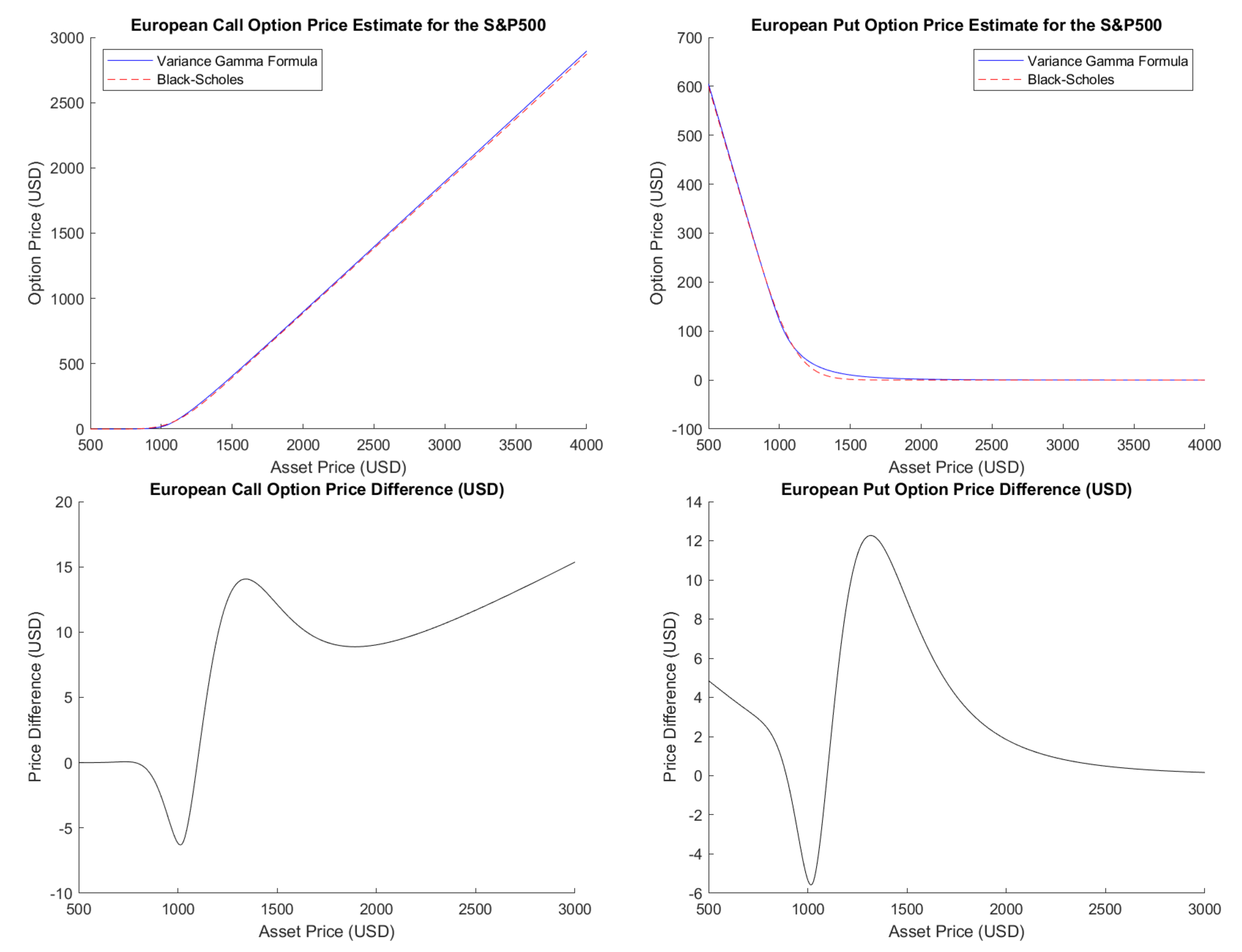
4.1. Variance Gamma Formula Values and Behavior

For the aforementioned comparison, we will use the values of European call options with the S&P500 as the underlying asset, bought at the close of the market on 18 April 2002. According to [23], at the close of the market on 18 April 2002, we had a risk-free rate of return $r=1.9\%$, a dividend rate of $q=1.2\%$, and the stock price closed at $S_0=1124.47$, with a volatility parameter, for the Black–Scholes model, of $\sigma =0.1812$ and risk neutral parameters $C=1.3574$, $G=5.8704$, and $M=14.2699$ for the Variance Gamma model.

We will take advantage of 75 actual recorded values that are presented in Table 1, and make an error estimation for each model, by calculating their respective root mean square error, which is given by the formula $RMSE=\sqrt{{\sum }_{i=1}^n{(\mathrm{market}{\mathrm{price}}_i-\mathrm{model}{\mathrm{price}}_i)}^2/n}$. Under this metric, Table 2 presents the deviations from the observed results.

Table 1. Table containing the values for the Variance Gamma Formula (49) for $n=22$, $m=27$, and $k=7$, denoted by “F”, the Monte Carlo method with 10000 simulated trajectories, denoted by “MC”, and the observed market values are denoted by “Real”.

	Time of Maturity
Strike	May			June			September			December			March			June			December
Price	2002			2002			2002			2002			2003			2003			2003
	F	MC	Real	F	MC	Real	F	MC	Real	F	MC	Real	F	MC	Real	F	MC	Real	F	MC	Real
975	152.76	151.72	-	156.80	156.19	-	166.83	168.05	161.60	176.13	176.13	173.30	184.76	183.79	-	192.81	194.67	-	207.41	206.05	-
995	133.42	132.40	-	138.17	137.60	-	149.64	150.82	144.80	159.98	160.09	157.00	169.40	168.42	-	178.07	179.85	182.10	193.65	192.31	-
1025	104.69	103.73	-	110.74	110.27	-	124.65	125.79	120.10	136.64	136.93	133.10	147.27	146.28	146.50	156.88	158.52	-	173.84	172.57	-
1050	81.09	80.20	-	88.49	88.16	84.50	104.71	105.81	100.70	118.12	118.59	114.80	129.75	128.65	-	140.10	141.69	143.00	158.15	156.92	171.40
1075	57.95	57.12	-	67.00	66.78	64.30	85.75	86.78	82.50	100.59	101.29	97.60	113.15	111.92	-	124.20	125.73	-	143.24	142.10	-
1090	44.39	43.58	43.10	54.58	54.41	-	74.92	75.90	-	90.59	91.42	-	103.68	102.36	-	115.11	116.57	-	134.67	133.62	-
1100	35.53	34.74	35.60	46.56	46.42	-	67.97	68.91	65.50	84.15	85.08	81.20	97.57	96.19	96.20	109.23	110.66	111.30	129.13	128.15	140.40
1110	26.88	26.12	-	38.79	38.69	39.50	61.25	62.16	-	77.92	78.92	-	91.65	90.18	-	103.52	104.91	-	123.71	122.81	-
1120	18.50	17.81	22.90	31.33	31.25	33.50	54.79	55.68	-	71.91	72.96	-	85.90	84.37	-	97.97	99.33	-	118.43	117.61	-
1125	14.47	13.82	20.20	27.74	27.69	30.70	51.66	52.54	51.00	68.98	70.07	66.90	83.10	81.54	81.70	95.25	96.61	97.00	115.84	115.07	-
1130	10.60	10.00	-	24.26	24.25	28.00	48.60	49.50	-	66.11	67.23	-	80.34	78.76	-	92.58	93.91	-	113.29	112.55	-
1135	7.09	6.53	-	20.93	20.93	25.60	45.63	46.45	45.50	63.30	64.45	-	77.63	76.04	-	89.94	91.26	-	110.76	110.07	-
1140	5.99	5.49	13.30	17.77	17.79	23.20	42.73	43.52	-	60.55	61.73	58.90	74.97	73.36	-	87.35	88.66	-	108.28	107.62	-
1150	4.66	4.26	-	12.55	12.60	19.10	37.20	37.92	38.10	55.23	56.44	53.90	69.81	68.17	68.30	82.30	83.58	83.30	103.40	102.81	112.80
1160	3.75	3.44	-	10.02	10.09	15.30	32.06	32.72	-	50.17	51.39	-	64.84	63.20	-	77.43	78.65	-	98.67	98.13	-
1170	3.08	2.82	-	8.24	8.32	12.10	27.37	27.96	-	45.38	46.59	-	60.09	58.46	-	72.72	73.88	-	94.07	93.58	-
1175	2.81	2.57	-	7.52	7.61	10.90	25.23	25.78	27.70	43.09	44.28	42.50	57.79	56.18	56.60	70.44	71.56	-	91.82	91.36	99.80
1200	1.82	1.68	-	4.93	5.06	-	17.15	17.54	19.60	32.79	33.78	33.00	47.14	45.62	46.10	59.70	60.65	60.90	81.11	80.74	-
1225	1.22	1.15	-	3.35	3.55	-	12.16	12.50	13.20	24.61	25.46	24.90	37.91	36.50	36.90	50.10	50.90	49.80	71.28	70.97	-
1250	0.84	0.80	-	2.34	2.53	-	8.79	9.12	-	18.59	19.29	18.30	30.17	28.88	29.30	41.67	42.34	41.20	62.30	62.03	66.90
1275	0.59	0.57	-	1.67	1.84	-	6.45	6.76	-	14.14	14.76	13.20	23.92	22.71	22.50	34.40	34.92	-	54.19	53.94	-
1300	0.42	0.41	-	1.20	1.34	-	4.79	5.08	-	10.84	11.40	-	18.96	17.90	17.20	28.24	28.59	27.10	46.90	46.63	49.50
1325	0.31	0.30	-	0.88	0.98	-	3.59	3.82	-	8.35	8.85	-	15.06	14.15	12.80	23.12	23.33	-	40.42	40.09	-
1350	0.23	0.22	-	0.65	0.71	-	2.71	2.92	-	6.47	6.88	-	11.99	11.23	-	18.92	19.01	17.10	34.71	34.31	35.70
1400	0.12	0.13	-	0.36	0.41	-	1.58	1.72	-	3.95	4.16	-	7.66	7.16	-	12.67	12.67	10.10	25.37	24.87	25.20
1450	0.07	0.09	-	0.21	0.24	-	0.95	1.03	-	2.45	2.55	-	4.95	4.62	-	8.51	8.46	-	18.42	17.69	17.00
1500	0.04	0.06	-	0.13	0.14	-	0.58	0.67	-	1.55	1.61	-	3.23	3.03	-	5.76	5.66	-	13.33	12.48	12.20

Table 2. Root Mean Square Error.

RMSE
Black–Scholes	6.6692
Variance Gamma Monte Carlo	3.9979
Variance Gamma Formula	3.7373

Therefore, not only is the Formula (49) more expedient due to much lower computational time, but it also outperforms the Monte-Carlo method (and, consequently, the Black–Scholes by a wide margin). From Figure 1, one can also observe that the formulas for the European options under the Variance Gamma (49) and (84) present typical behavior. For example, a change in the initial asset price influences the price formula as one would expect, yet with some substantial differences from the Black–Scholes model.

Figure 1. European Options prices under the Black–Scholes and Variance Gamma models and their differences, for $K=1100$, $\tau =35\times 7/365$ and different values of $S_0$.

Let us note that, in [23], the author estimates the model parameters and calculates the option prices for the same option data and the same Variance Gamma model while using the Fast Fourier transform method of [7], and it obtains a RMSE value of $3.56$, which is a little smaller than the one we obtained. We have also calculated the RMSE by the same numerical method and we obtained a RMSE of $3.74$. These small discrepancies are perhaps a result of small differences in the precise computation of the maturities of some options.

More importantly the Formula (49) also displays the volatility smile typically present in most assets, with values relatively close to the empirical observed on present asset, as can be seen from Figure 2.

Figure 2. Implied Volatility for the empirical data and Black–Scholes and Variance Gamma models, where $S_0=1124.47$, $K=1100$, and $\tau =35\times 7/365$.

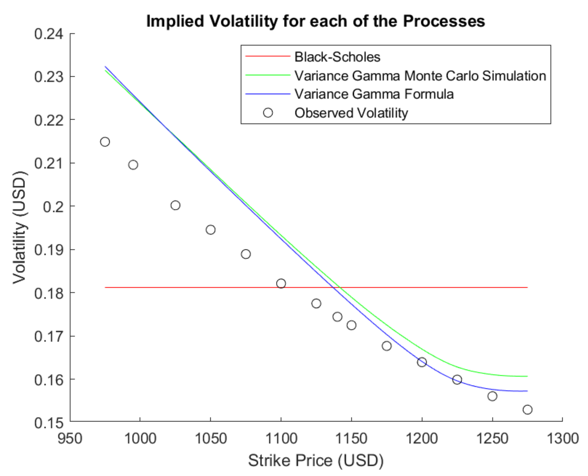
4.2. Convergence of the Variance Gamma Formula

In order to study the numerical convergence and precision of the new formula, we must first realize that observing the value of each isolated term in the triple sum (49) is fallacious, since an unit increase of, for instance, parameter n will lead to the sum of an extra $m\times k$ terms, which may lead to an error of substantially higher magnitude than each individual term. Let us denote each term of the sum (49) by $C_{VG}(n,m,k)$. Given this notation, we can write $C_{VG}={\sum }_{n=0}^{\infty }{\sum }_{m=0}^{\infty }{\sum }_{k=0}^{\infty }{C}_{VG}(n,m,k)$. To determine the values $n_{\max }$, $m_{\max }$, and $k_{\max }$, for which the sum $C_{VG}$ converges, for all values K and $\tau$ of Table 1, we will apply the Euclidean norm to the 189 resulting values from the three possible double sum series: the series computed by summing the terms of $C_{VG}$ for a fixed n and $0\le m,k\le n$, i.e., $C_{VG}^{\mathrm{n}\mathrm{const}}\left(n\right)={\sum }_{m=0}^n{\sum }_{k=0}^n{C}_{VG}(n,m,k)$, the series computed by summing the terms of $C_{VG}$ for a fixed m and $0\le n,k\le m$, i.e., $C_{VG}^{\mathrm{m}\mathrm{const}}\left(m\right)={\sum }_{n=0}^m{\sum }_{k=0}^m{C}_{VG}(n,m,k)$, and the series computed by summing the terms of $C_{VG}$ for a fixed k and $0\le n,m\le k$, i.e., $C_{VG}^{\mathrm{k}\mathrm{const}}\left(k\right)={\sum }_{n=0}^k{\sum }_{m=0}^k{C}_{VG}(n,m,k)$.

From the values shown in Table 3, for any K and $\tau$ of Table 1, we can assure convergence with a two-decimal precision, when the sum of the three double sum series has a result lower than 0.005, for instance, $n=22$, $m=27$, and $k=7$.

Table 3. Convergence of the three double series.

	Double Series Sum				Double Series Sum
	${\mathit{C}}_{\mathit{VG}}^{\mathit{n}\mathbf{const}}$ (n)	${\mathit{C}}_{\mathit{VG}}^{\mathit{m}\mathbf{const}}$ (m)	${\mathit{C}}_{\mathit{VG}}^{\mathit{k}\mathbf{const}}$ (k)		${\mathit{C}}_{\mathit{VG}}^{\mathit{n}\mathbf{const}}$ (n)	${\mathit{C}}_{\mathit{VG}}^{\mathit{m}\mathbf{const}}$ (m)	${\mathit{C}}_{\mathit{VG}}^{\mathit{k}\mathbf{const}}$ (k)
0	1573.462	1573.462	1573.462	14	3.451	5.456	0.000
1	942.085	1624.942	93.249	15	1.263	2.653	0.000
2	1473.360	2138.478	14.602	16	0.430	1.277	0.000
3	396.878	2185.591	0.656	17	0.137	0.609	0.000
4	530.501	1834.503	0.121	18	0.041	0.288	0.000
5	350.999	1328.181	0.008	19	0.011	0.135	0.000
6	358.913	862.780	0.001	20	0.003	0.063	0.000
7	287.068	518.316	0.000	21	0.001	0.029	0.000
8	214.182	294.406	0.000	22	0.000	0.013	0.000
9	139.772	160.554	0.000	23	0.000	0.006	0.000
10	81.751	84.932	0.000	24	0.000	0.003	0.000
11	42.733	43.875	0.000	25	0.000	0.001	0.000
12	20.221	22.236	0.000	26	0.000	0.001	0.000
13	8.716	11.090	0.000	27	0.000	0.000	0.000

Let us note that, in [20,22], the authors studied the convergence of their double series for the option price with a ${10}^{-3}$ precision, while considering the price of a single European call option (with fixed maturity and strike) under the fractional diffusion process and the finite moment Lévy stable process. They have concluded that is enough to sum the terms in the series up to $n=6$ and $m=6$. The results are quite different, because, in their models the call option price is given by a double series (not a triple series), the convergence was estimated for a single option (we calculate the convergence for options of all maturities and strikes in our data set), and their underlying model is not the Variance Gamma model.

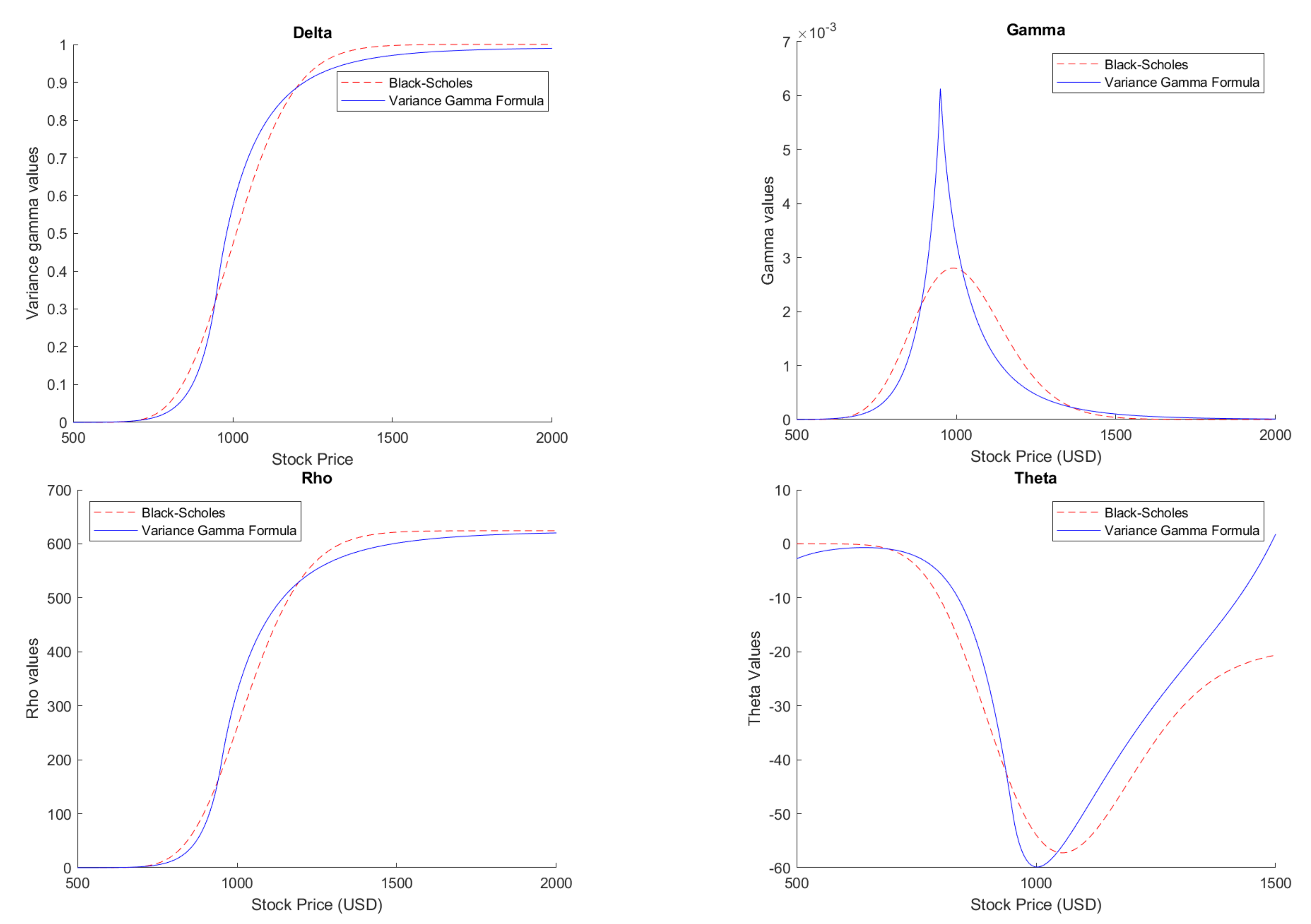
4.3. The Greek Formulas Behavior

We terminate this section by visualizing and contrasting the behavior of Greek functions under the two models. The Greek functions for the Variance Gamma model seem similar enough to the ones of the Black–Scholes model, yet they exhibit enough discrepancies to be worthy of note, primarily in the behavior of the Gamma and Theta functions, as can be seen in Figure 3. These discrepancies can have important consequences in establishing hedging strategies and the associated expected profit and loss. We refer to [22] for a detailed discussion of this subject in the case of the finite moment log-stable model.

Figure 3. Greek functions under the Black–Scholes and Variance Gamma models, for $K=1100$ and $\tau =35\times 7/365$.

Furthermore, while some greek functions properties, such as ${\Delta }_C,{\mathrm{\Gamma }}_C,{\rho }_C,-{\Theta }_C>0$, can be difficult to prove analytically from the Formulas (85), (89), (93), and (94), one can easily observe their validity, by generating the graphs of Figure 3 for a variety of different values of S, K, r, q and $\tau$.

5. Conclusions

We have derived a triple Mellin–Barnes integral representation for the price of a European call option in a market model where a Variance Gamma process drives the price of the underlying asset. Subsequently, we applied the multidimensional residue calculus to the aforementioned integral and computed a triple sum series for the European call option price (49). Triple sum series for the delta, gamma, rho, and theta Greeks were also found by direct differentiation. When numerically tested, Formula (49) exhibited the behavior that was typically observed in the market for European options, and it outperformed the Monte-Carlo simulation method in both accuracy and computational time. The Greeks also displayed their usual behavior.

For practical applications, the simplicity of the aforementioned formulas (such as the lack of necessity of simulations for pricing European options, or of complex numerical schemes to compute the Greeks), coupled with their higher rates of precision and much lower computation time, makes them ideal for financial practitioners. For example, Formulas (85) and (89) can be used directly to generate a portfolio with optimal delta and gamma hedge strategies.

In terms of future research, the most obvious course of action would be to compare the performance of Formula (49), in terms of accuracy and computational time, to other semi-closed formulas such as the Bessel functions representation formula or the Fast Fourier Transform method for the price of a European call option under the Variance Gamma model (as discussed in [6,7]).

In terms of generalization of the theoretical results, the more pressing question will be the ability to use a similar reasoning to that presented in Section 3 to arrive at a sum series for the more general CGMY process and Generalized Tempered Stable process, even if this necessitates a higher dimensional Mellin–Barnes integral. One also might inquire further into the pricing of more complex financial instruments, like American or Barrier options, and especially instruments like Asian options, where the integral that is involved in their definition seems to make them a prime candidate for residue calculus.

References

- Black, F.; Scholes, M. The pricing of options and Corporate Liabilities. J. Political Econ. 1973, 81, 637–654. [Google Scholar] [CrossRef]
- Merton, R.C. The Theory of Rational Option Pricing. Bell J. Econ. Manag. Sci. 1973, 4, 141–183. [Google Scholar] [CrossRef]
- Fama, E.F. The Behavior of Stock-Market Prices. J. Bus. 1965, 38, 34–105. [Google Scholar] [CrossRef]
- Madan, D.B.; Seneta, E. The Variance Gamma (V.G.) Model for Share Market Returns. J. Bus. 1990, 63, 511–524. [Google Scholar] [CrossRef]
- Mandelbrot, B. The Variation of Certain Speculative Prices. J. Bus. 1963, 36, 394–419. [Google Scholar] [CrossRef]
- Madan, D.B.; Carr, P.P.; Chang, E.C. The Variance Gamma Process and Option Pricing. Rev. Financ. 1998, 2, 79–105. [Google Scholar] [CrossRef]
- Carr, P.; Madan, D.B.; Stanley, M. Option valuation using the Fast Fourier Transform. J. Comput. Financ. 1999, 2, 61–73. [Google Scholar] [CrossRef]
- Fang, F.; Oosterlee, C.W. A Novel Pricing Method for European Options Based on Fourier-Cosine Series Expansions. SIAM J. Sci. Comput. 2008, 31, 826–848. [Google Scholar] [CrossRef]
- Cont, R.; Voltchkova, E. A Finite Difference Scheme for Option Pricing in Jump Diffusion and Exponential Lévy Models. SIAM J. Numer. Anal. 2005, 43, 1596–1626. [Google Scholar] [CrossRef]
- Cantarutti, N.; Guerra, J. Multinomial method for option pricing under Variance Gamma. Int. J. Comput. Math. 2019, 96, 1087–1106. [Google Scholar] [CrossRef]
- Sato, K.I. Lévy Processes and Infinitely Divisible Distributions; Cambridge University Press: Cambridge, UK, 1999. [Google Scholar]
- Carr, P.; Wu, L. The finite moment log stable process and option pricing. J. Financ. 2003, 58, 753–777. [Google Scholar] [CrossRef]
- Mainardi, F.; Luchko, Y.; Pagnini, G. The Fundamental Solution of the Space-Time Fractional Diffusion Equation. 2007. Available online: https://arxiv.org/abs/cond-mat/0702419 (accessed on 25 March 2021).
- Gorenflo, R.; Luchko, Y.; Mainardi, F. Analytical Properties and Applications of the Wright Function. 2007. Available online: https://arxiv.org/abs/math-ph/0701069v1 (accessed on 25 March 2021).
- Mainardi, F. Fractional Calculus: Some Basic Problems in Continuum and Statistical Mechanics. In Fractals and Fractional Calculus in Continuum Mechanics; International Centre for Mechanical Sciences (Courses and Lectures); Carpinteri, A., Mainardi, F., Eds.; Springer: Vienna, Austria, 1997; pp. 291–348. [Google Scholar] [CrossRef]
- Gorenflo, R.; Mainardi, F.; Raberto, M.; Scalas, E. Fractional diffusion in finance: Basic theory. In Proceedings of the MDEF2000-Workshop ‘Modelli Dinamici in Economia e Finanza’, Urbino, Italy, 28–30 September 2000. [Google Scholar]
- Passare, M.; Tsikh, A.; Zhdanov, O. A multidimensional Jordan residue lemma with an application to Mellin-Barnes integrals. In Contributions to Complex Analysis and Analytic Geometry; Skoda, H., Trépreau, J.M., Eds.; Vieweg+Teubner Verlag: Wiesbaden, Germany, 1994. [Google Scholar]
- Passare, M.; Tsikh, A.; Cheshel, A. Multiple Mellin-Barnes integrals as periods of Calabi-Yau manifolds with several moduli. Theor. Math. Phys. 1996, 109, 1544–1555. [Google Scholar] [CrossRef]
- Zhdanov, O.; Tsikh, A. Studying the multiple Mellin-Barnes integrals by means of multidimensional residues. Sib. Math. J. 1998, 39, 245–260. [Google Scholar] [CrossRef]
- Aguilar, J.P.; Coste, C.; Korbel, J. Series representation of the pricing formula for the European option driven by space-time fractional diffusion. Fract. Calc. Appl. Anal. 2018, 21, 981–1004. [Google Scholar] [CrossRef]
- Aguilar, J.P.; Korbel, J. Option pricing models driven by the space-time fractional diffusion: Series representation and applications. Fractal Fract. 2018, 2, 15. [Google Scholar] [CrossRef]
- Aguilar, J.P.; Korbel, J. Simple formulas for pricing and hedging European options in the finite moment log-stable model. Risks 2019, 7, 36. [Google Scholar] [CrossRef]
- Schoutens, W. Lévy Processes in Finance: Pricing Financial Derivatives; Wiley: Hoboken, NJ, USA, 2003. [Google Scholar] [CrossRef]
- Griffiths, P.; Harris, J. Principles of Algebraic Geometry; Wiley Online Library: Hoboken, NJ, USA, 1978. [Google Scholar] [CrossRef]
- Begehr, H.G.; Dzhuraev, A.; Begher, H. An Introduction to Several Complex Variables and Partial Differential Equations; Addison-Wesley Longman: Harlow, UK, 1997. [Google Scholar]
- Titchmarsh, E.C. Introduction to the Theory of Fourier Integrals; The Clarendon Press: Oxford, UK, 1937. [Google Scholar]
- Abramowitz, M.; Stegun, I.A. Handbook of Mathematical Functions with Formulas, Graphs, and Mathematical Tables, 9th dover printing, 10th gpo printing ed.; Dover: New York, NY, USA, 1964. [Google Scholar]
- Cont, R.; Tankov, P. Financial Modelling with Jump Processes; Chapman and Hall/CRC Financial Mathematics Series; CRC Press: Boca Raton, FL, USA, 2003. [Google Scholar] [CrossRef]
Publisher’s Note: MDPI stays neutral with regard to jurisdictional claims in published maps and institutional affiliations. |
© 2021 by the authors. Licensee MDPI, Basel, Switzerland. This article is an open access article distributed under the terms and conditions of the Creative Commons Attribution (CC BY) license (https://creativecommons.org/licenses/by/4.0/).