Nonlinear-Observer-Based Design Approach for Adaptive Event-Driven Tracking of Uncertain Underactuated Underwater Vehicles

Abstract

A nonlinear-observer-based design methodology is proposed for an adaptive event-driven output-feedback tracking problem with guaranteed performance of uncertain underactuated underwater vehicles (UUVs) in six-degrees-of-freedom (6-DOF). A nonlinear observer using adaptive neural networks is presented to estimate the velocity information in the presence of unknown nonlinearities in the dynamics of 6-DOF UUVs where a state transformation approach using a time-varying scaling factor is introduced. Then, an output-feedback tracker using a nonlinear error function and estimated states is recursively designed to overcome the underactuated problem of the system dynamics and to guarantee preselected control performance in three-dimensional space. It is shown that the tracking error of the nonlinear-observer-based output-feedback control system exponentially converges a small neighbourhood around the zero. Efficiency of the resulting output-feedback strategy is verified through a simulation.

1. Introduction

Over the past few decades, the development of advanced control strategies has stimulated interest in the control field of autonomous underwater vehicles [1]. The design and control techniques of autonomous underwater vehicles were surveyed in [2]. Several study results have been presented for various control problems of autonomous underwater vehicles such as subsea cable tracking using magnetic sensing guidance [3], control in remote and hostile environments [4], chemical plume tracing [5], path following using Lagrange multipliers [6], and survey, inspection and intervention of Girona 500 [7]. Initial research has focused on the two-dimensional horizontal or vertical tracking control problems of autonomous underwater vehicles. In [8], an adaptive nonlinear controller was designed for depth control of autonomous underwater vehicles on the vertical plane. In [9], a combined problem of trajectory planning and tracking control was addressed for underactuated underwater vehicles (UUVs) on the horizontal plane. A terminal sliding mode control approach was proposed for the trajectory tracking of UUVs on the horizontal plane [10]. In [11], a Lyapunov-based model predictive control design was developed for fully-actuated underwater vehicles on the horizontal plane. A robust backstepping controller using the time delay estimation was proposed for fully-actuated underwater vehicles [12]. These results [8,9,10,11,12] are only available for the two-dimensional tracking control of autonomous underwater vehicles.

To deal with more practical underwater environments, the control problems in three-dimensional underwater space were addressed for autonomous underwater vehicles. In [13], a three-dimensional path following a control problem was addressed for 5-degrees-of-freedom (5-DOF) UUVs in the presence of ocean current. In [14], an ocean current observer design was presented for three-dimensional trajectory tracking of 5-DOF UUVs. Function approximation methods using neural networks have been applied to design adaptive trackers of 5-DOF UUVs. A command filtered backstepping control approach using neural networks was developed for uncertain 5-DOF UUVs [15]. In [16], a neural-network-based target tracking problem was investigated for uncertain 5-DOF UUVs. The tracking control problems of uncertain 6-DOF underwater vehicles have been addressed using several control approaches such as neural-network-based adaptive control [17], hierarchical robust nonlinear control [18], and hybrid tracking control [19]. Furthermore, predefined performance control designs have recently been developed for uncertain 6-DOF underwater vehicles. In [20], a tracking controller using performance functions was presented for uncertain 6-DOF UUVs. A neural-network-based target tracking control problem with a prescribed performance was considered for uncertain 6-DOF UUVs [21]. In [22], an adaptive region tracking control problem with prescribed transient performance was addressed fully-actuated 6-DOF underwater vehicles with thruster fault. An event-triggered neural network tracking control design with predefined performance was developed for uncertain 6-DOF UUVs [23]. Despite these successful results, full state measurements are required in the aforementioned tracking designs, that is, all positions and velocities of underwater vehicles should be measured online. Owing to the economic cost and other limitations, underwater vehicles may not be equipped with velocity sensors, or the velocity measurements can be easily corrupted by sensor noises.

To design the controller independent of the velocity sensors, some output-feedback control designs have been developed of underwater vehicles. Due to the existence of rotational matrices for linear and angular velocities in the kinematics, the observer design problem to estimate velocity information has been regarded as a challenging problem in the output-feedback tracking field of 5-DOF or 6-DOF underwater vehicles. In [24], an output-feedback controller using nonlinear Luenberger observers was designed for 5-DOF slender-body underwater vehicles. In [25], an output-feedback control law for 5-DOF UUVs without model uncertainties was designed by using sliding mode observer and backstepping technique. A linear-observer-based adaptive control strategy was suggested for fully-actuated 6-DOF underwater vehicles [26]. In [27], a neural-network-based robust tracker using a prescribed performance technique and a high-gain observer was designed for fully-actuated 6-DOF underwater vehicles. However, the aforementioned works [24,25,26,27] did not consider the model of 6-DOF UUVs for the design of the output-feedback tracking controllers. Besides, the continuously updated tracking laws reported in [24,25,26,27] cannot be efficiently operated in the network-based underwater environment with low propagation speed, capacity-limited bandwidth and high energy consumption. To manage the transmission signal data economically, some limited studies have tried to deal with the event-triggered full state-feedback design problems for the depth control of underwater vehicles [28] and the prescribed performance control of 6-DOF UUVs [23]. Although these results [23,28] provide some remedies on the event-triggered tracking problems of underwater vehicles, they require the measurement of all state variables of underwater vehicles. To the best of our observations, there is no systematic solution available for the output-feedback event-triggered tracking of uncertain 6-DOF UUVs. The adaptive velocity observer design problem of uncertain 6-DOF UUVs especially still remains unaddressed in the control field of underwater vehicles.

In this work, we present an adaptive-nonlinear-observer-based design methodology for event-driven output-feedback tracking with guaranteed performance of uncertain 6-DOF UUVs in three-dimensional space. Specifically, the term ‘output-feedback event-triggered tracking’ means that the position information of the UUV is only measured to design the controller of the UUV, which is intermittently updated when an event-triggering condition is satisfied. Thus, the term ‘adaptive velocity observer design’ indicates that the velocity observer using the adaptive neural network approximator is designed to estimate the unmeasurable velocity information of the UUV. Our design consists of the following steps. Firstly, to estimate velocity information in the presence of unknown nonlinear functions in the dynamics of UUVs, an adaptive velocity observer using state transformation and neural networks is developed by deriving adaptive tuning laws based on a scaling function. Secondly, by employing the error transformation technique using a rotation matrix, a guaranteed-performance-based event-triggered output-feedback control scheme and its triggering law are constructed to operate uncertain 6-DOF UUVs stably within the pre-designated error region. Furthermore, the dynamics of auxiliary variables are introduced to overcome the underactuated property of underwater vehicles in the tracker design and stability analysis. Finally, simulation results are provided to verify the effectiveness of the proposed theoretical result.

Compared with the related results in the literature, the proposed novelties are two-fold.

(i)

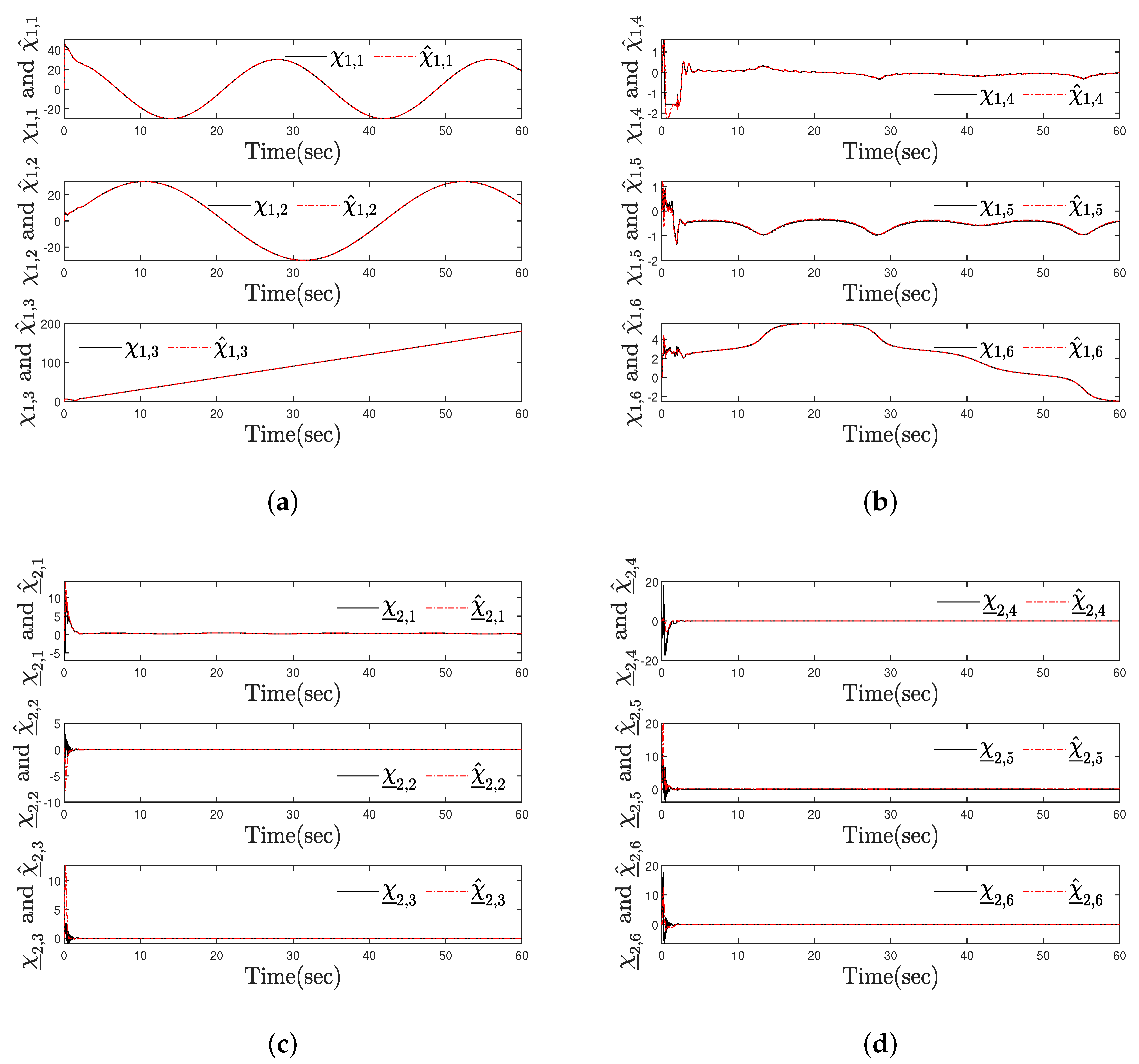
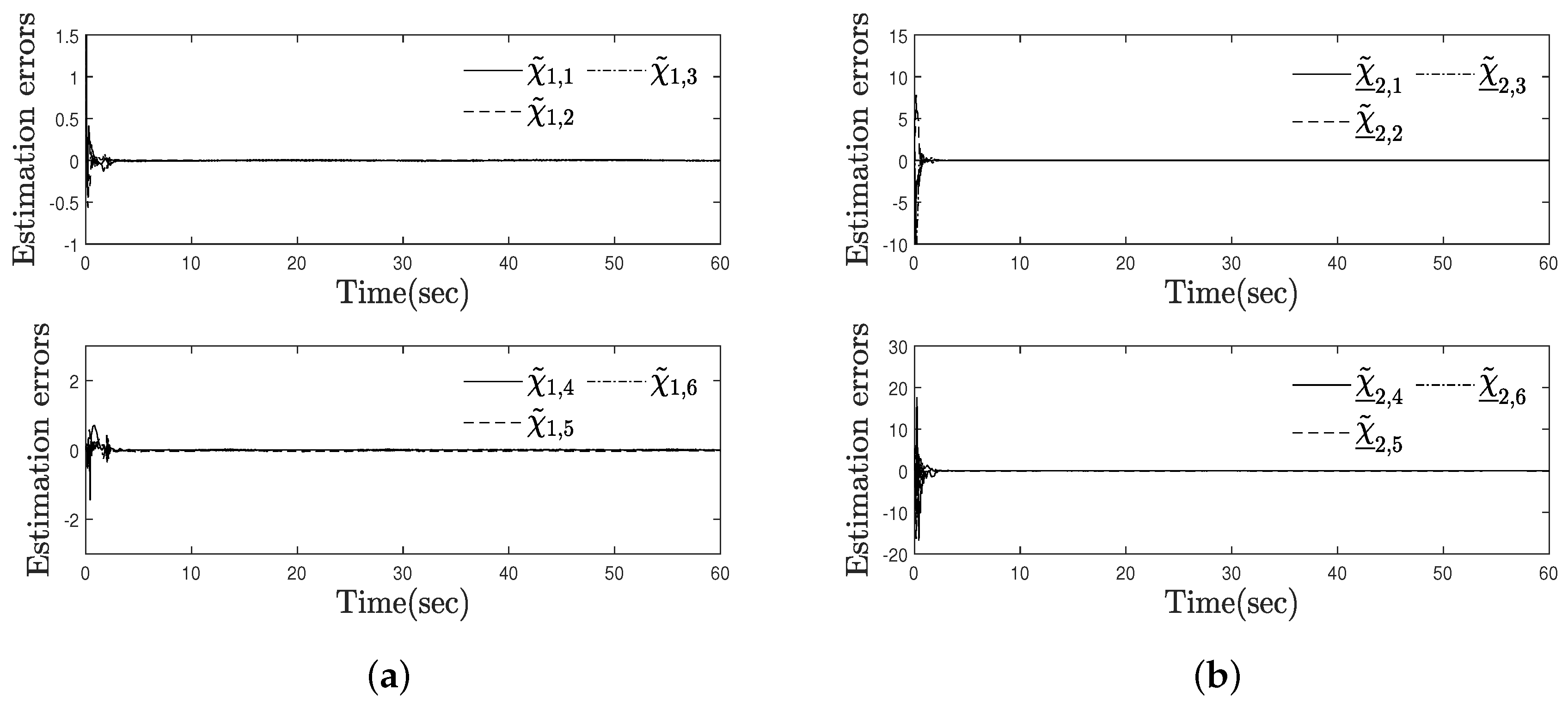
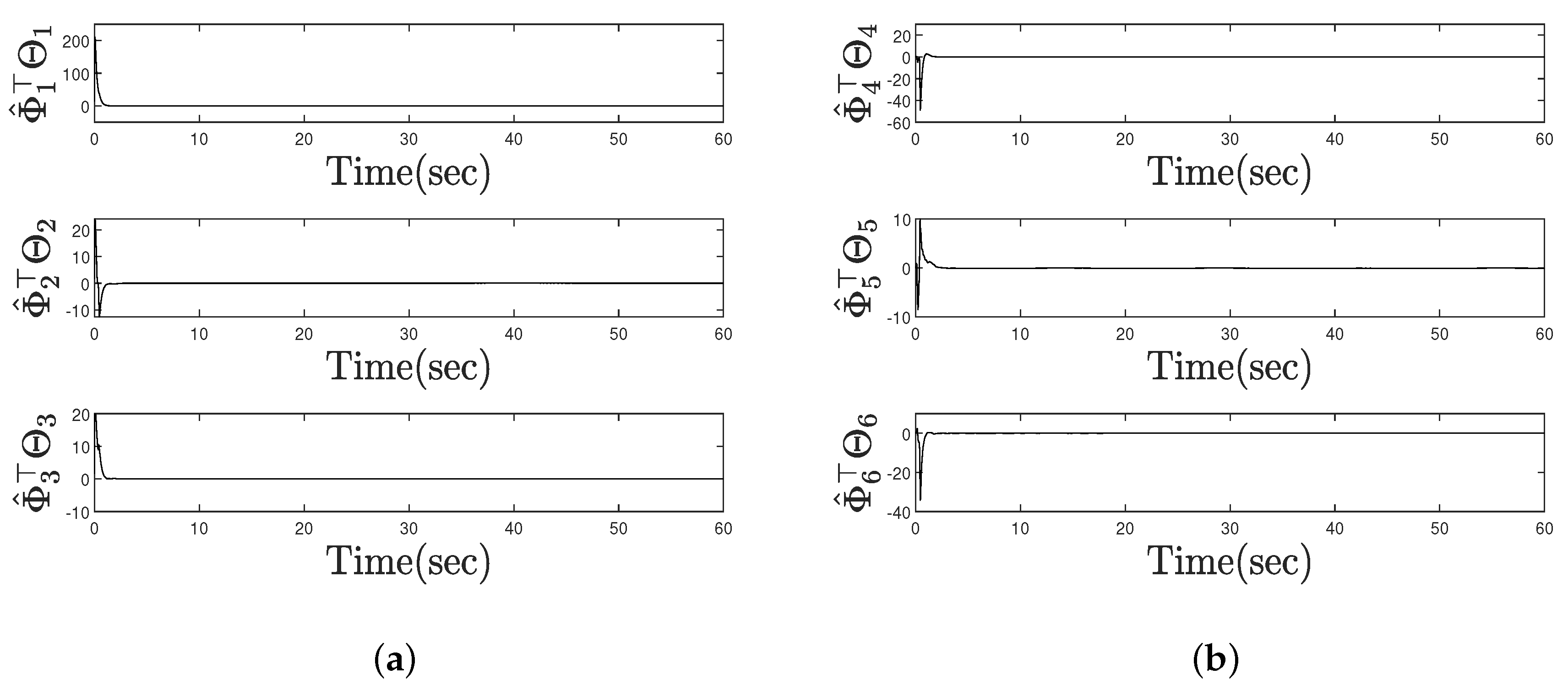
Contrary to the existing output-feedback tracking methods for 5-DOF or 6-DOF underwater vehicles [24,25,26,27], this study considers unknown system nonlinearities of the 6-DOF UUV dynamics. Thus, an adaptive velocity observer design strategy using state transformation and neural networks is proposed to estimate the velocity information of UUVs while compensating for the unknown system nonlinearities, where adaptive laws based on a scaling function are derived to learn weights of neural networks.

(ii)

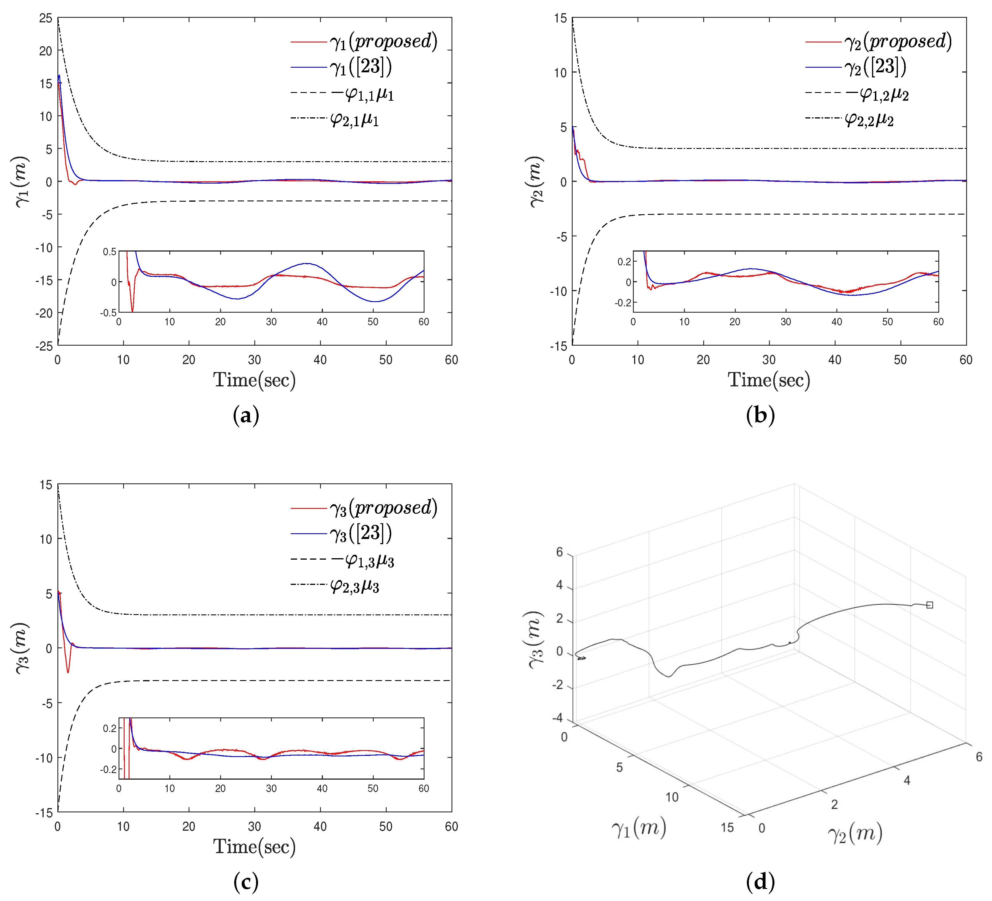
Compared with the existing event-triggered control results for three-dimensional tracking [23,28], this study establishes the design methodology of the guaranteed-performance-based adaptive tracker and its event-triggering condition depending on only the position measurement of 6-DOF UUVs. Then, the stability of the proposed output-feedback event-triggered tracking system is analyzed in the Lyapunov sense.

The remaining part of this paper is structured as follows: The event-driven output-feedback tracking problem is formulated in Section 2. In Section 3, the adaptive-nonlinear-observer-based design methodology for event-driven output-feedback tracking with guaranteed performance and stability analysis is presented. In Section 4, simulation results are provided. Finally, a conclusion is drawn in Section 5.

2. Problem Formulation

We consider the kinematic and dynamic equations of a 6-DOF UUV represented by

$$\begin{array}{cc}\hfill & \begin{array}{c}\dot{\beta }=R_1\left(\zeta \right)\upsilon \hfill \\ \dot{\zeta }=R_2\left(\zeta \right)\omega \hfill \end{array}\hfill \end{array}$$

(1)

$$\begin{array}{cc}\hfill & M\left[\begin{array}{c}\dot{\upsilon }\\ \dot{\omega }\end{array}\right]=D(\upsilon ,\omega )+B\left(\zeta \right)+\eta ,\hfill \end{array}$$

(2)

where $\beta ={[x,y,z]}^{\top }$ and $\zeta ={[\varphi ,\theta ,\psi ]}^{\top }$; (x, y, z) and ($\varphi$, $\theta$, $\psi$) denote the positions (i.e., surge, sway and heave displacements) and orientations (i.e., roll, pitch, and yaw angles) of the UUV, respectively, $\upsilon ={[u,v,w]}^{\top }$ and $\omega ={[p,q,r]}^{\top }$; (u, v, w) and (p, q, r) are the position velocities (i.e., surge, sway, and heave velocities) and orientation velocities (i.e., roll, pitch, and yaw angular velocities) of the UUV, respectively, $R_1\left(\zeta \right)$ and $R_2\left(\zeta \right)$ are the rotation matrix for the linear velocity and the transformation matrix for the angular velocity, respectively, defined as

$$\begin{array}{cc}\hfill & R_1\left(\zeta \right)=\left[\begin{array}{ccc}{c}_{\theta }{c}_{\psi }& s_{\theta }{c}_{\psi }{s}_{\varphi }-s_{\psi }{c}_{\varphi }& s_{\theta }{c}_{\psi }{c}_{\varphi }+s_{\psi }{s}_{\varphi }\\ c_{\theta }{s}_{\psi }& s_{\theta }{s}_{\psi }{s}_{\varphi }+c_{\psi }{c}_{\varphi }& s_{\theta }{s}_{\psi }{c}_{\varphi }-c_{\psi }{s}_{\varphi }\\ -s_{\theta }& c_{\theta }{s}_{\varphi }& c_{\theta }{c}_{\varphi }\end{array}\right],\hfill \\ \hfill & R_2\left(\zeta \right)=\left[\begin{array}{ccc}1& t_{\theta }{s}_{\varphi }& t_{\theta }{c}_{\varphi }\\ 0& c_{\varphi }& -s_{\varphi }\\ 0& s_{\varphi }/c_{\theta }& c_{\varphi }/c_{\theta }\end{array}\right],\hfill \end{array}$$

with $s_{(·)}\triangleq sin(·)$, $c_{(·)}\triangleq cos(·)$, and $t_{(·)}\triangleq tan(·)$, M denotes the mass and inertial matrix, $D(\upsilon ,\omega )\in {\mathbb{R}}^6$ is a vector related to the Coriolis and damping matrices, $B\left(\zeta \right)\in {\mathbb{R}}^6$ is a hydrostatic vector of the UUV, and from the moving property of the torpedo-shaped UUV [29], $\eta$ is defined as the underacutated torque vector $\eta =[{\eta }_X,0,0,0,{\eta }_M,{\eta }_N]$. In this work, the underacutated control vector $\eta$ is intermittently updated according to the triggering law to be derived later. The nonlinearities M, D, and B in the dynamics of the UUV are taken from the definitions reported in [23,30,31]. The structure of the neutrally buoyant UUV concerned in this study is depicted in Figure 1.

Assumption 1.

In three-dimensional space, the desired trajectory ${\beta }_d\in {\mathbb{R}}^3$ and its time derivatives ${\dot{\beta }}_d\in {\mathbb{R}}^3$ and ${\ddot{\beta }}_d\in {\mathbb{R}}^3$ are bounded.

Assumption 2.

The system nonlinearities $D(\upsilon ,\omega )$ and $B\left(\zeta \right)$ are assumed to be unknown.

Assumption 3.

The positions β and orientations ζ are only measurable. That is, the velocity vectors υ and ω are unmeasurable.

The primary objective of this paper is to design an adaptive-observer-based event-driven output-feedback tracking law $\eta$ without velocity measurements for the uncertain 6-DOF nonlinear UUV (i.e., (1) and (2)) while guaranteeing predesignated tracking performance in three-dimensional space.

3. Nonlinear-Observer-Based Design Approach for Event-Driven Output- Feedback Control

3.1. Adaptive Nonlinear Observer Design Using Neural Networks

In this section, the neural-network-based adaptive observer with state transformation is developed to estimate the velocity information in the presence of unknown nonlinear functions of the UUV dynamics. For our adaptive observer design, a state transformation is presented as

$$\begin{array}{c}\hfill {\underline{\chi }}_2=\Omega {\chi }_2,\end{array}$$

(3)

where ${\underline{\chi }}_2={[{\underline{\chi }}_{2,1},\dots ,{\underline{\chi }}_{2,6}]}^{\top }$, ${\chi }_2={[{\chi }_{2,1},\dots ,{\chi }_{2,6}]}^{\top }={[{\upsilon }^{\top },{\omega }^{\top }]}^{\top }$ and a time-varying scaling signal $\Omega \in \mathbb{R}$ is provided by the differential equation $\dot{\Omega }=-(L_2+\parallel R^{\top }{\parallel }^2/4)\Omega +L_3$ with $\Omega \left(0\right)>0$, constants $L_2>0$ and $L_3>0$, and $R=\mathrm{diag}[R_1,R_2]$. By using (3), the kinematics (1) and the dynamics (2) of the UUV are transformed as

$$\begin{array}{cc}\hfill {\dot{\chi }}_1=& {\Omega }^{-1}R{\underline{\chi }}_2\hfill \\ \hfill {\dot{\underline{\chi }}}_2=& -\left(L_2+\frac{\parallel R^{\top }{\parallel }^2}{4}\right){\underline{\chi }}_2+R^{\top }F({\chi }_1,{\underline{\chi }}_2)+\Omega M^{-1}\eta \hfill \end{array}$$

(4)

where ${\chi }_1={[{\chi }_{1,1},\dots ,{\chi }_{1,6}]}^{\top }={[{\beta }^{\top },{\zeta }^{\top }]}^{\top }$ and $F={\left(R^{\top }\right)}^{-1}[L_3{\Omega }^{-1}{\underline{\chi }}_2+\Omega M^{-1}(D\left({\Omega }^{-1}{\underline{\chi }}_2\right)+B\left({\chi }_1\right))]$.

By employing a universal function approximation technique using neural networks, the unknown continuous function F can be approximated by radial basis function neural networks as follows [32]:

$$F\left(\overline{x}\right)={\mathsf{\Phi }}^{\top }\Theta \left(\overline{x}\right)+\epsilon \left(\overline{x}\right),$$

(5)

where $\overline{x}={[{\chi }_1^{\top },{\underline{\chi }}_2^{\top }]}^{\top }\in \Xi \subset {\mathbb{R}}^{12}$ denotes the input vector, $\mathsf{\Phi }=\mathrm{diag}[{\mathsf{\Phi }}_1,\dots ,{\mathsf{\Phi }}_6]$ is the optimal weighting matrix satisfying ${\parallel \mathsf{\Phi }\parallel }_F\le \overline{\mathsf{\Phi }}$ with an unknown positive constant $\overline{\mathsf{\Phi }}$, ${\mathsf{\Phi }}_j={[{\mathsf{\Phi }}_{j,1},\dots ,{\mathsf{\Phi }}_{j,n}]}^{\top }$ with $j=1,\dots ,6$, the Frobenius norm is defined as ${\parallel ·\parallel }_F$, $\Theta$ is the vector of the Gaussian function $\Theta ={[{\Theta }_1^{\top },\dots ,{\Theta }_6^{\top }]}^{\top }$; ${\Theta }_j={[{\Theta }_{j,1},\dots ,{\Theta }_{j,n}]}^{\top }$ with $j=1,\dots ,6$, and $\epsilon \in {\mathbb{R}}^6$ is a reconstruction error vector bounded as $\parallel \epsilon \parallel \le \overline{\epsilon }$ with an unknown positive constant $\overline{\epsilon }$.

Lemma 1.

[33] For the Gaussian function vector Θ, there exists a constant $\overline{\Theta }>0$ such that $\parallel \Theta \parallel \le \overline{\Theta }$.

The adaptive observer using radial basis function neural networks is designed as

$$\begin{array}{cc}\hfill {\dot{\widehat{\chi }}}_1=& {\Omega }^{-1}R{\underline{\widehat{\chi }}}_2+L_1{\tilde{\chi }}_1\hfill \\ \hfill {\dot{\widehat{\underline{\chi }}}}_2=& -\left(L_2+\frac{\parallel R^{\top }{\parallel }^2}{4}\right){\widehat{\underline{\chi }}}_2+R^{\top }{\widehat{\mathsf{\Phi }}}^{\top }\Theta \left(\widehat{\overline{x}}\right)+{\Omega }^{-1}{R}^{\top }{\tilde{\chi }}_1+\varpi +\Omega M^{-1}\eta ,\hfill \end{array}$$

(6)

where ${\widehat{\chi }}_1$ and ${\widehat{\underline{\chi }}}_2$ are the estimates of ${\chi }_1$ and ${\underline{\chi }}_2$, respectively, $\widehat{\overline{x}}={[{\widehat{\chi }}_1^{\top },{\widehat{\underline{\chi }}}_2^{\top }]}^{\top }$, ${\tilde{\chi }}_1={\chi }_1-{\widehat{\chi }}_1$, $L_1$ is the positive constant denoting the observer gain, $\varpi$ is an auxiliary term to be determined in the controller design procedure, and $\widehat{\mathsf{\Phi }}$ is the estimate of $\mathsf{\Phi }$ and is tuned by the following adaptation law:

$$\begin{array}{cc}\hfill {\widehat{\mathsf{\Phi }}}_j=& {\delta }_j(\Omega {\Theta }_j\left(\widehat{\overline{x}}\right){\tilde{\chi }}_1^{\top }+\Gamma )\hfill \\ \hfill \dot{\Gamma }=& -\Omega {\dot{\Theta }}_j\left(\widehat{\overline{x}}\right){{\tilde{\chi }}_1}^{\top }-\dot{\Omega }{\Theta }_j\left(\widehat{\overline{x}}\right){{\tilde{\chi }}_1}^{\top }+\Omega L_1{\Theta }_j\left(\widehat{\overline{x}}\right){{\tilde{\chi }}_1}^{\top }-{\sigma }_j{\widehat{\mathsf{\Phi }}}_j,\hfill \end{array}$$

(7)

where $j=1,\dots ,6$, ${\delta }_j=\mathrm{diag}[{\delta }_{j,1},\dots ,{\delta }_{j,n}]>0$; ${\delta }_{j,l}>0$, $l=1,\dots ,n$, is a constant, and $0<{\sigma }_j<2$ is a constant for $\sigma$-modification.

The observer error dynamics along (4)–(6) is obtained as

$$\begin{array}{cc}\hfill {\dot{\tilde{\chi }}}_1=& {\Omega }^{-1}R{\underline{\tilde{\chi }}}_2-L_1{\tilde{\chi }}_1\hfill \\ \hfill {\dot{\tilde{\underline{\chi }}}}_2=& -\left(L_2+\frac{\parallel R^{\top }{\parallel }^2}{4}\right){\tilde{\underline{\chi }}}_2+R^{\top }({\mathsf{\Phi }}^{\top }\Theta \left(\overline{x}\right)-{\widehat{\mathsf{\Phi }}}^{\top }\Theta \left(\widehat{\overline{x}}\right)+\epsilon )-{\Omega }^{-1}{R}^{\top }{\tilde{\chi }}_1-\varpi ,\hfill \end{array}$$

(8)

where ${\tilde{\underline{\chi }}}_2={\underline{\chi }}_2-{\widehat{\underline{\chi }}}_2$.

For the adaptive observer, we define a Lyapunov function candidate as

$$\begin{array}{cc}\hfill V_o& =\frac{1}{2}[{{\tilde{\chi }}_1}^{\top }{\tilde{\chi }}_1+{{\tilde{\underline{\chi }}}_2}^{\top }{\tilde{\underline{\chi }}}_2+tr\left({\tilde{\mathsf{\Phi }}}^{\top }{\delta }^{-1}\tilde{\mathsf{\Phi }}\right)],\hfill \end{array}$$

(9)

where $V_o$ is a positive definite function and $\tilde{\mathsf{\Phi }}=\mathsf{\Phi }-\widehat{\mathsf{\Phi }}$.

In (8), we have that

$$\begin{array}{c}\hfill {\mathsf{\Phi }}^{\top }\Theta \left(\overline{x}\right)-{\widehat{\mathsf{\Phi }}}^{\top }\Theta \left(\widehat{\overline{x}}\right)={\tilde{\mathsf{\Phi }}}^{\top }\Theta \left(\widehat{\overline{x}}\right)+{\mathsf{\Phi }}^{\top }(\Theta \left(\overline{x}\right)-\Theta \left(\widehat{\overline{x}}\right)).\end{array}$$

(10)

By substituting (8) into ${\dot{V}}_o$ and using (7) and (10), ${\dot{V}}_o$ becomes

$$\begin{array}{cc}\hfill {\dot{V}}_o=& -L_1{{\tilde{\chi }}_1}^{\top }{\tilde{\chi }}_1-\left(L_2+\frac{\parallel R^{\top }{\parallel }^2}{4}\right){{\tilde{\underline{\chi }}}_2}^{\top }{\tilde{\underline{\chi }}}_2+{{\tilde{\underline{\chi }}}_2}^{\top }{R}^{\top }\{{\mathsf{\Phi }}^{\top }(\Theta \left(\overline{x}\right)-\Theta \left(\widehat{\overline{x}}\right))+\epsilon \}\hfill \\ \hfill & -{{\tilde{\underline{\chi }}}_2}^{\top }\varpi +{\sigma }_{j}tr\left({\tilde{\mathsf{\Phi }}}^{\top }\widehat{\mathsf{\Phi }}\right)\hfill \\ \hfill \le & -L_1{{\tilde{\chi }}_1}^{\top }{\tilde{\chi }}_1-\left(L_2+\frac{\parallel R^{\top }{\parallel }^2}{4}\right){{\tilde{\underline{\chi }}}_2}^{\top }{\tilde{\underline{\chi }}}_2-{{\tilde{\underline{\chi }}}_2}^{\top }\varpi +{\sigma }_{j}tr\left({\tilde{\mathsf{\Phi }}}^{\top }\widehat{\mathsf{\Phi }}\right)+\frac{\parallel {\tilde{\underline{\chi }}}_2{\parallel }^2{\parallel R^{\top }\parallel }^2}{4}\hfill \\ \hfill & +\parallel {\mathsf{\Phi }}^{\top }(\Theta \left(\overline{x}\right)-\Theta \left(\widehat{\overline{x}}\right)){+\epsilon \parallel }^2.\hfill \end{array}$$

(11)

From Lemma 1, we have $\parallel {\mathsf{\Phi }}^{\top }(\Theta \left(\overline{x}\right)-\Theta \left(\widehat{\overline{x}}\right))\parallel <2\overline{\mathsf{\Phi }}\overline{\Theta }$. Then, owing to $\parallel \epsilon \parallel \le \overline{\epsilon }$, there exists a constant $\iota$ such that $\parallel {\mathsf{\Phi }}^{\top }(\Theta \left(\overline{x}\right)-\Theta \left(\widehat{\overline{x}}\right)){+\epsilon \parallel }^2\le \iota$.

In addition, the term ${\sigma }_{j}tr\left({\tilde{\mathsf{\Phi }}}^{\top }\widehat{\mathsf{\Phi }}\right)$ in (11) becomes

$$\begin{array}{cc}\hfill {\sigma }_{j}tr\left({\tilde{\mathsf{\Phi }}}^{\top }\widehat{\mathsf{\Phi }}\right)=& {\sigma }_{j}tr\left({\tilde{\mathsf{\Phi }}}^{\top }(\mathsf{\Phi }-\tilde{\mathsf{\Phi }})\right)\hfill \\ \hfill \le & -{\sigma }_{j}tr\left({\tilde{\mathsf{\Phi }}}^{\top }\tilde{\mathsf{\Phi }}\right)+\frac{{\sigma }_j^2}{2}{\parallel \tilde{\mathsf{\Phi }}\parallel }_F^2+\frac{{\overline{\mathsf{\Phi }}}^2}{2}\hfill \\ \hfill \le & -\overline{{\sigma }_j}{\parallel \tilde{\mathsf{\Phi }}\parallel }_F^2+\frac{{\overline{\mathsf{\Phi }}}^2}{2},\hfill \end{array}$$

(12)

where $\overline{{\sigma }_j}={\sigma }_j(1-{\sigma }_j/2)$ is strictly positive because of $0<{\sigma }_j<2$.

Substituting (12) into (11) gives

$$\begin{array}{cc}\hfill {\dot{V}}_o\le & -L_1{{\tilde{\chi }}_1}^{\top }{\tilde{\chi }}_1-L_2{{\tilde{\underline{\chi }}}_2}^{\top }{\tilde{\underline{\chi }}}_2-{{\tilde{\underline{\chi }}}_2}^{\top }\varpi -\overline{{\sigma }_j}{\parallel \tilde{\mathsf{\Phi }}\parallel }_F+\frac{{\overline{\mathsf{\Phi }}}^2}{2}+{\iota }^2.\hfill \end{array}$$

(13)

Remark 1.

Compared with the existing works [23,24,25,26,27,28], we design the neural-network-based adaptive observer (6) to estimate the unmeasurable velocities of the UUV. To this end, the transformed velocity variable (3) is presented to derive the adaptive laws (7) dependent on the position error ${\tilde{\chi }}_1$ in the presence of unknown nonlinearities of the dynamics. In addition, the term ϖ in (6) is designed to deal with the coupling term between the error dynamics of the observer and controller in the Lyapunov-based stability analysis.

3.2. Output-Feedback Event-Driven Controller Design and Stability Analysis

Based on the estimated velocity information, a guaranteed-performance-based output-feedback event-driven control methodology is established via a nonlinear error function with a time-varying bounding function and some auxiliary signals. The dynamic surface design technique [34] is employed for the recursive output-feedback control design. The controller design is based on the Lyapunov stability theorem.

Step 1: The position error vector is defined as $\gamma ={[{\gamma }_1,{\gamma }_2,{\gamma }_3]}^{\top }=\beta -{\beta }_d$. To achieve the guaranteed performance of the position error vector, a nonlinear error function ${\mathsf{{\rm Y}}}_1={[{\mathsf{{\rm Y}}}_{1,1},{\mathsf{{\rm Y}}}_{1,2},{\mathsf{{\rm Y}}}_{1,3}]}^{\top }$ is presented as

$$\begin{array}{c}\hfill {\mathsf{{\rm Y}}}_1=R_1^{-1}\left(\zeta \right)\Lambda -\mu ,\end{array}$$

(14)

where $\mu ={[{\mu }_1,0,0]}^{\top }$ is a design constant denoting an acceptable radius of the error surface and $\Lambda ={[{\Lambda }_1,{\Lambda }_2,{\Lambda }_3]}^{\top }$; the nonlinear functions ${\Lambda }_i$, $i=1,2,3$, are defined as

$$\begin{array}{c}\hfill {\Lambda }_i\left(\frac{{\gamma }_i}{{\rho }_i}\right)=ln\left(\frac{{\phi }_{1,i}{\phi }_{2,i}+{\phi }_{2,i}({\gamma }_i/{\rho }_i)}{{\phi }_{1,i}{\phi }_{2,i}-{\phi }_{1,i}({\gamma }_i/{\rho }_i)}\right),\end{array}$$

(15)

where ${\rho }_i\left(t\right)=({\rho }_{i,0}-{\rho }_{i,\infty })e^{-g_{i}t}+{\rho }_{i,\infty }$; $g_i$, ${\rho }_{i,0}$, and ${\rho }_{i,\infty }$ are positive design parameters satisfying ${\rho }_{i,0}>{\rho }_{i,\infty }$ and $-{\phi }_{1,i}{\rho }_i\left(0\right)<{\gamma }_i\left(0\right)<{\phi }_{2,i}{\rho }_i\left(0\right)$, and ${\phi }_{1,i}$ and ${\phi }_{2,i}$ are design constants such that $0<{\phi }_{1,i},{\phi }_{2,i}\le 1$.

Lemma 2.

[23] It is satisfied that $-{\phi }_{1,i}{\rho }_i\left(t\right)<{\gamma }_i\left(t\right)<{\phi }_{2,i}{\rho }_i\left(t\right)$, $\forall t>0$ provided that ${\mathsf{{\rm Y}}}_{1,i}\in {\mathcal{L}}_{\infty }$ where $i=1,2,3$.

Remark 2.

The nonlinear error transformation (14) using the rotation matrix $R_1^{-1}\left(\zeta \right)$ and the design constant is employed to guarantee that the three-dimensional trajectory error γ remains within the predesignated time-varying bounds. Namely, the guaranteed performance of the proposed output-feedback event-driven tracking system (i.e., $-{\phi }_{1,i}{\rho }_i\left(t\right)<{\gamma }_i\left(t\right)<{\phi }_{2,i}{\rho }_i\left(t\right)$, $\forall t\ge 0$) is obtained in three-dimensional space. Lemma 2 shows that the boundedness of the nonlinear error function $Y_1$ implies the guaranteed performance. To achieve our control objective, we design the estimated-states-based underactuated control vector η to guarantee the boundedness of ${\mathsf{{\rm Y}}}_{1,i}$.

From (14) and $\dot{\beta }=R_{1}v$, differentiating ${\mathsf{{\rm Y}}}_1$ with respect to time yields

$$\begin{array}{cc}\hfill {\dot{\mathsf{{\rm Y}}}}_1=& -N({\mathsf{{\rm Y}}}_1+\mu )+R_1^{-1}H(R_{1}v-{\dot{\beta }}_d-\dot{\rho }{\rho }^{-1}\gamma ),\hfill \end{array}$$

(16)

where $H=\mathrm{diag}[H_1,H_2,H_3]$ with $H_i=(1/\left({\gamma }_i+{\phi }_{1,i}{\rho }_i\right))-(1/\left({\gamma }_i-{\phi }_{2,i}{\rho }_i\right))$, $i=1,2,3$, $\rho =\mathrm{diag}[{\rho }_1,{\rho }_2,{\rho }_3]$, $\mathrm{diag}[·]$ indicates the diagonal matrix, and

$$\begin{array}{c}\hfill N=-{\dot{R}}_1^{-1}{R}_1=\left[\begin{array}{ccc}0& -r& q\\ r& 0& -p\\ -q& p& 0.\end{array}\right].\end{array}$$

(17)

By defining $Q=R_1^{-1}H{R}_1$ and using (17) and the definition ${[{\chi }_{2,1},\dots ,{\chi }_{2,6}]}^{\top }={[{\upsilon }^{\top },{\omega }^{\top }]}^{\top }$, ${\dot{\mathsf{{\rm Y}}}}_1$ becomes

$$\begin{array}{cc}\hfill {\dot{\mathsf{{\rm Y}}}}_1& =-N{\mathsf{{\rm Y}}}_1-\left[\begin{array}{ccc}0& -{\chi }_{2,6}& {\chi }_{2,5}\\ {\chi }_{2,6}& 0& -{\chi }_{2,4}\\ -{\chi }_{2,5}& {\chi }_{2,4}& 0\end{array}\right]\left[\begin{array}{c}{\mu }_1\\ 0\\ 0\end{array}\right]+Q\left[\begin{array}{c}{\chi }_{2,1}\\ {\chi }_{2,2}\\ {\chi }_{2,3}\end{array}\right]-R_1^{-1}H({\dot{\beta }}_d+\dot{\rho }{\rho }^{-1}\gamma )\hfill \\ \hfill & =-N{\mathsf{{\rm Y}}}_1+K\left[\begin{array}{c}{\chi }_{2,1}\\ {\chi }_{2,5}\\ {\chi }_{2,6}\end{array}\right]+Q\left[\begin{array}{c}0\\ {\chi }_{2,2}\\ {\chi }_{2,3}\end{array}\right]-R_1^{-1}H({\dot{\beta }}_d+\dot{\rho }{\rho }^{-1}\gamma ),\hfill \end{array}$$

(18)

where

$$\begin{array}{c}\hfill K=\left[\begin{array}{ccc}{Q}_{1,1}& 0& 0\\ Q_{2,1}& 0& -{\mu }_1\\ Q_{3,1}& {\mu }_1& 0.\end{array}\right].\end{array}$$

Here, $Q_{1,1}$, $Q_{2,1}$, and $Q_{3,1}$ are the (1,1), (2,1), and (3,1) components of Q.

Applying the state transformation (3) and the observer errors ${\tilde{\underline{\chi }}}_{2,i}={\underline{\chi }}_{2,i}-{\widehat{\underline{\chi }}}_{2,i}$, $i=1,\dots ,6$ to (18) gives

$$\begin{array}{cc}\hfill {\dot{\mathsf{{\rm Y}}}}_1=& -N{\mathsf{{\rm Y}}}_1+K_{\Omega }\left(\left[\begin{array}{c}{\widehat{\underline{\chi }}}_{2,1}\\ {\widehat{\underline{\chi }}}_{2,5}\\ {\widehat{\underline{\chi }}}_{2,6}\end{array}\right]+\left[\begin{array}{c}{\tilde{\underline{\chi }}}_{2,1}\\ {\tilde{\underline{\chi }}}_{2,5}\\ {\tilde{\underline{\chi }}}_{2,6}\end{array}\right]\right)+Q_{\Omega }\left(\left[\begin{array}{c}0\\ {\widehat{\underline{\chi }}}_{2,2}\\ {\widehat{\underline{\chi }}}_{2,3}\end{array}\right]+\left[\begin{array}{c}0\\ {\tilde{\underline{\chi }}}_{2,2}\\ {\tilde{\underline{\chi }}}_{2,3}\end{array}\right]\right)\hfill \\ \hfill & -R_1^{-1}H({\dot{\beta }}_d+\dot{\rho }{\rho }^{-1}\gamma ),\hfill \end{array}$$

(19)

where $K_{\Omega }={\Omega }^{-1}K$ and $Q_{\Omega }={\Omega }^{-1}Q$.

Then, the error surface s is defined as $s={[s_u,s_q,s_r]}^{\top }$ where $s_u={\widehat{\underline{\chi }}}_{2,1}-{\overline{\varsigma }}_u$, $s_q={\widehat{\underline{\chi }}}_{2,5}-{\overline{\varsigma }}_q$, and $s_r={\widehat{\underline{\chi }}}_{2,6}-{\overline{\varsigma }}_r$. Here, ${\overline{\varsigma }}_u$, ${\overline{\varsigma }}_q$, and ${\overline{\varsigma }}_r$ are the filtered signals of the virtual control laws ${\varsigma }_u$, ${\varsigma }_q$, and ${\varsigma }_r$, respectively, and are provided by the following first-order low-pass filter

$$\begin{array}{c}\alpha \dot{\overline{\varsigma }}+\overline{\varsigma }=\varsigma ,\overline{\varsigma }\left(0\right)=\varsigma \left(0\right),\hfill \end{array}$$

(20)

where $\overline{\varsigma }={[{\overline{\varsigma }}_u,{\overline{\varsigma }}_q,{\overline{\varsigma }}_r]}^{\top }$, $\varsigma ={[{\varsigma }_u,{\varsigma }_q,{\varsigma }_r]}^{\top }$, and $\alpha >0$ is the small positive constant. Then, the boundary layer error vector is defined as $c=[c_1,c_2,c_3]=\overline{\varsigma }-\varsigma$.

By applying the error vectors s and c to (19), ${\dot{\mathsf{{\rm Y}}}}_1$ is represented by

$$\begin{array}{cc}\hfill {\dot{\mathsf{{\rm Y}}}}_1=& -N{\mathsf{{\rm Y}}}_1+K_{\Omega }\left(\left[\begin{array}{c}{\tilde{\underline{\chi }}}_{2,1}\\ {\tilde{\underline{\chi }}}_{2,5}\\ {\tilde{\underline{\chi }}}_{2,6}\end{array}\right]+s+\varsigma +c\right)+Q_{\Omega }\left(\left[\begin{array}{c}0\\ {\widehat{\underline{\chi }}}_{2,2}\\ {\widehat{\underline{\chi }}}_{2,3}\end{array}\right]+\left[\begin{array}{c}0\\ {\tilde{\underline{\chi }}}_{2,2}\\ {\tilde{\underline{\chi }}}_{2,3}\end{array}\right]\right)\hfill \end{array}$$

$$\begin{array}{c}\hfill -R_1^{-1}H({\dot{\beta }}_d+\dot{\rho }{\rho }^{-1}\gamma ).\end{array}$$

(21)

We design the virtual control vector $\varsigma$ as

$$\begin{array}{c}\hfill \varsigma =K_{\Omega }^{-1}\left(-{\kappa }_1{\mathsf{{\rm Y}}}_1-Q_{\Omega }\left[\begin{array}{c}0\\ {\widehat{\underline{\chi }}}_{2,2}\\ {\widehat{\underline{\chi }}}_{2,3}\end{array}\right]+R_1^{-1}H({\dot{\beta }}_d+\dot{\rho }{\rho }^{-1}\gamma )\right),\end{array}$$

(22)

where ${\kappa }_1=\mathrm{diag}\left[{\kappa }_{1,1}{\kappa }_{1,2}{\kappa }_{1,3}\right]$ with constants ${\kappa }_{1,i}>0$, $i=1,2,3$.

The Lyapunov function is considered as $V_{c,1}={\mathsf{{\rm Y}}}_1^{\top }{\mathsf{{\rm Y}}}_1/2$ where $V_{c,1}$ is a positive definite function. Using (22), ${\dot{V}}_{c,1}$ is obtained as

$$\begin{array}{cc}\hfill {\dot{V}}_{c,1}& =-{\mathsf{{\rm Y}}}_1^{\top }{\kappa }_1{\mathsf{{\rm Y}}}_1+{\mathsf{{\rm Y}}}_1^{\top }{K}_{\Omega }({[{\tilde{\underline{\chi }}}_{2,1},{\tilde{\underline{\chi }}}_{2,5},{\tilde{\underline{\chi }}}_{2,6}]}^{\top }+s+c)+{\mathsf{{\rm Y}}}_1^{\top }{Q}_{\Omega }{[0,{\tilde{\underline{\chi }}}_{2,2},{\tilde{\underline{\chi }}}_{2,3}]}^{\top },\hfill \end{array}$$

(23)

where the skew symmetric property of the matrix N is used for ${\mathsf{{\rm Y}}}_1^{\top }N{\mathsf{{\rm Y}}}_1=0$.

Step 2: In this step, the event-driven underactuated control law $\eta =[{\eta }_X,0,0,0,{\eta }_M,{\eta }_N]$ is designed to stabilize the error surface vector ${\mathsf{{\rm Y}}}_2={[{\mathsf{{\rm Y}}}_{2,1},\dots ,{\mathsf{{\rm Y}}}_{2,6}]}^{\top }={\widehat{\underline{\chi }}}_2-U$ where $U={[{\overline{\varsigma }}_u,{\tau }_1,{\tau }_2,{\tau }_3,{\overline{\varsigma }}_q,{\overline{\varsigma }}_r]}^{\top }$. Here, ${\tau }_1$, ${\tau }_2$, and ${\tau }_3$ denote the auxiliary variables to deal with the underactuated property of $\eta$.

From (6), ${\dot{\mathsf{{\rm Y}}}}_2$ is represented by

$$\begin{array}{cc}\hfill {\dot{\mathsf{{\rm Y}}}}_2& =\varrho +\Omega M^{-1}\eta -\dot{U},\hfill \end{array}$$

(24)

where $\varrho =-(L_2+(\parallel R^{\top }{\parallel }^2/4\left)\right){\widehat{\underline{\chi }}}_2+R^{\top }{\widehat{\mathsf{\Phi }}}^{\top }\Theta \left(\widehat{\overline{x}}\right)+{\Omega }^{-1}{R}^{\top }{\tilde{\chi }}_1+\varpi$. An adaptive output-feedback event-driven tracker $\eta \left(t\right)$ is designed as

$$\begin{array}{cc}\hfill \eta \left(t\right)=& \breve{\eta }\left(t_a\right),\forall t\in [t_a,t_{a+1})\hfill \end{array}$$

(25)

$$\begin{array}{cc}\hfill t_{a+1}=& \inf \{t>t_a|\parallel E_{\eta }\left(t\right)\parallel \ge A_1\parallel s\left(t\right)\parallel +A_2\},\hfill \end{array}$$

(26)

where $E_{\eta }\left(t\right)=\Omega (\breve{\eta }\left(t\right)-\eta \left(t\right))$, $a\in {\mathbb{Z}}^{+}$, $t_a$ means the ath event time of the tracking law $\eta$, and $A_1>0$ and $A_2>0$ are design constants. According to the triggering law (26), the control law $\eta$ is updated and set to $\breve{\eta }={[{\breve{\eta }}_1,0,0,0,{\breve{\eta }}_5,{\breve{\eta }}_6]}^{\top }$. Here, ${\breve{\eta }}_1$, ${\breve{\eta }}_5$, and ${\breve{\eta }}_6$ are selected as

$$\begin{array}{cc}\hfill \left[\begin{array}{c}{\breve{\eta }}_1\\ {\breve{\eta }}_5\\ {\breve{\eta }}_6\end{array}\right]=& \frac{1}{\Omega }\left(-{\overline{\kappa }}_{2,1}s-\left[\begin{array}{c}{\left(M\varrho \right)}_1\\ {\left(M\varrho \right)}_5\\ {\left(M\varrho \right)}_6\end{array}\right]+\left[\begin{array}{c}{\left(M\dot{U}\right)}_1\\ {\left(M\dot{U}\right)}_5\\ {\left(M\dot{U}\right)}_6\end{array}\right]-K_{\Omega }^{\top }{\mathsf{{\rm Y}}}_1-A_1\left[\begin{array}{c}{\mathsf{{\rm Y}}}_{2,1}\\ {\mathsf{{\rm Y}}}_{2,5}\\ {\mathsf{{\rm Y}}}_{2,6}\end{array}\right]-A_{2}tanh\left(\frac{s}{\vartheta }\right)\right),\hfill \end{array}$$

(27)

where ${\overline{\kappa }}_{2,1}=\mathrm{diag}[{\kappa }_{2,1},{\kappa }_{2,5},{\kappa }_{2,6}]$ with design constants ${\kappa }_{2,1}>0$, ${\kappa }_{2,5}>0$, and ${\kappa }_{2,6}>0$, ${(·)}_l$ is the lth row of $(·)$, $tanh(s/\vartheta )={[tanh({\mathsf{{\rm Y}}}_{2,1}/\vartheta ),tanh({\mathsf{{\rm Y}}}_{2,5}/\vartheta ),tanh({\mathsf{{\rm Y}}}_{2,6}/\vartheta )]}^{\top }$ with a positive constant $\vartheta$, and $\dot{U}={[({\varsigma }_u-{\overline{\varsigma }}_u)/\alpha ,{\dot{\tau }}_1,{\dot{\tau }}_2,{\dot{\tau }}_3,({\varsigma }_q-{\overline{\varsigma }}_q)/\alpha ,({\varsigma }_r-{\overline{\varsigma }}_r)/\alpha ]}^{\top }$. Here, ${\tau }_1$, ${\tau }_2$, and ${\tau }_3$ are obtained by

$$\begin{array}{cc}\hfill \left[\begin{array}{c}{\dot{\tau }}_1\\ {\dot{\tau }}_2\\ {\dot{\tau }}_3\end{array}\right]=& {\overline{M}}_2^{-1}\left({\overline{\kappa }}_{2,2}\left[\begin{array}{c}{\mathsf{{\rm Y}}}_{2,2}\\ {\mathsf{{\rm Y}}}_{2,3}\\ {\mathsf{{\rm Y}}}_{2,4}\end{array}\right]-{\overline{M}}_1\left[\begin{array}{c}({\varsigma }_u-{\overline{\varsigma }}_u)/\alpha \\ ({\varsigma }_q-{\overline{\varsigma }}_q)/\alpha \\ ({\varsigma }_r-{\overline{\varsigma }}_r)/\alpha \end{array}\right]+\left[\begin{array}{c}{\left(M\varrho \right)}_2\\ {\left(M\varrho \right)}_3\\ {\left(M\varrho \right)}_4\end{array}\right]\right),\hfill \end{array}$$

(28)

where ${\overline{\kappa }}_{2,2}=\mathrm{diag}[{\kappa }_{2,2},{\kappa }_{2,3},{\kappa }_{2,4}]$ with design constants ${\kappa }_{2,2}>0$, ${\kappa }_{2,3}>0$, and ${\kappa }_{2,4}>0$ and

$$\begin{array}{cc}\hfill {\overline{M}}_1& =\left[\begin{array}{ccc}0& 0& m{x}_g-Y_{\dot{r}}\\ 0& -m{x}_g-z_{\dot{q}}& 0\\ 0& 0& 0\end{array}\right]\hfill \\ \hfill {\overline{M}}_2& =\left[\begin{array}{ccc}m-Y_{\dot{v}}& 0& -m{z}_g\\ 0& m-Z_{\dot{w}}& m{y}_g\\ -m{z}_g& m{y}_g& I_{xx}-K_{\dot{p}}.\end{array}\right].\hfill \end{array}$$

The parameters in ${\overline{M}}_1$ and ${\overline{M}}_2$ are defined in the definition of M reported in [23].

The Lyapunov function candidate $V_{c,2}$ is selected as $V_{c,2}={\mathsf{{\rm Y}}}_2^{\top }M{\mathsf{{\rm Y}}}_2/2$ where $V_{c,2}$ is a positive definite function. Then, the time derivative of $V_{c,2}$ along (24) and the definition of $E_{\eta }$ is given by

$$\begin{array}{cc}\hfill {\dot{V}}_{c,2}& ={\mathsf{{\rm Y}}}_2^{\top }(M\varrho +\Omega \breve{\eta }-E_{\eta })-{\mathsf{{\rm Y}}}_2^{\top }M\dot{U}.\hfill \end{array}$$

(29)

By defining ${\overline{E}}_{\eta }={[{\breve{\eta }}_1-{\eta }_X,{\breve{\eta }}_5-{\eta }_M,{\breve{\eta }}_6-{\eta }_N]}^{\top }$, we have ${\mathsf{{\rm Y}}}_2^{\top }{E}_{\eta }=s^{\top }{\overline{E}}_{\eta }$ owing to $\parallel E_{\eta }\parallel =\parallel {\overline{E}}_{\eta }\parallel$. In addition, ${\mathsf{{\rm Y}}}_2^{\top }M\dot{U}$ is expressed by

$$\begin{array}{c}\hfill {\mathsf{{\rm Y}}}_2^{\top }M\dot{U}={\mathsf{{\rm Y}}}_2^{\top }\left[\begin{array}{c}{\left(M\dot{U}\right)}_1\\ 0\\ 0\\ 0\\ {\left(M\dot{U}\right)}_5\\ {\left(M\dot{U}\right)}_6\end{array}\right]+{\mathsf{{\rm Y}}}_2^{\top }\left[\begin{array}{c}0\\ {\overline{M}}_1\left[\begin{array}{c}({\varsigma }_u-{\overline{\varsigma }}_u)/\alpha \\ ({\varsigma }_q-{\overline{\varsigma }}_q)/\alpha \\ ({\varsigma }_r-{\overline{\varsigma }}_r)/\alpha \end{array}\right]+{\overline{M}}_2\left[\begin{array}{c}{\dot{\tau }}_1\\ {\dot{\tau }}_2\\ {\dot{\tau }}_3\end{array}\right]\\ 0\\ 0\end{array}\right].\end{array}$$

(30)

From the property $E_{\eta }\left(t_a\right)=0$ for $a\in {\mathbb{Z}}^{+}$ and the condition (26) for input triggering, $-{\mathsf{{\rm Y}}}_2^{\top }{E}_{\eta }\le \parallel s\parallel (A_1\parallel s\parallel +A_2)$ is satisfied. Then, using (27) and (28) yields

$$\begin{array}{cc}\hfill {\dot{V}}_{c,2}\le & -{\mathsf{{\rm Y}}}_2^{\top }{\kappa }_2{\mathsf{{\rm Y}}}_2+\parallel s\parallel A_2-A_2{s}^{\top }tanh\left(\frac{s}{\vartheta }\right)-s^{\top }{K}_{\Omega }^{\top }{\mathsf{{\rm Y}}}_1,\hfill \end{array}$$

(31)

where ${\kappa }_2=\mathrm{diag}[{\kappa }_{2,1},\dots ,{\kappa }_{2,6}]$. Using the inequality $0\le \parallel s\parallel -s^{\top }tanh(s/\vartheta )\le 0.8355\vartheta$, ${\dot{V}}_{c,2}$ is obtained as

$$\begin{array}{cc}\hfill {\dot{V}}_{c,2}\le & -{\mathsf{{\rm Y}}}_2^{\top }{\kappa }_2{\mathsf{{\rm Y}}}_2-s^{\top }{K}_{\Omega }^{\top }{\mathsf{{\rm Y}}}_1+0.8355A_2\vartheta .\hfill \end{array}$$

(32)

Differentiating the boundary layer error c with respect to time yields

$$\begin{array}{c}\hfill \dot{c}=-\frac{1}{\alpha }c+O({\mathsf{{\rm Y}}}_1,{\mathsf{{\rm Y}}}_2,c,\widehat{\mathsf{\Phi }},{\beta }_0),\end{array}$$

(33)

where ${\beta }_0={[{\beta }_d^{\top },{\dot{\beta }}_d^{\top },{\ddot{\beta }}_d^{\top }]}^{\top }$ and $$\begin{gathered} O={\dot{K}}_{\Omega }^{-1}\{-{\kappa }_1{\mathsf{{\rm Y}}}_1-Q_{\Omega }{[0,{\widehat{\underline{\chi }}}_{2,2},{\widehat{\underline{\chi }}}_{2,3}]}^{\top }+R_1^{-1}H({\dot{\beta }}_d+{\rho }^{-1}\dot{\rho }{\gamma }_1)\}+K_{\Omega }^{-1} \\ \{-{\kappa }_1\dot{\mathsf{{\rm Y}}}-Q_{\Omega }{[0,{\dot{\widehat{\underline{\chi }}}}_{2,2},{\dot{\widehat{\underline{\chi }}}}_{2,2}]}^{\top }-{\dot{Q}}_{\Omega }{[0,{\widehat{\underline{\chi }}}_{2,2},{\widehat{\underline{\chi }}}_{2,3}]}^{\top }+{\dot{R}}_1^{-1}H({\dot{\beta }}_d+{\rho }^{-1}\dot{\rho }{\gamma }_1) \\ +R_1^{-1}\dot{H}({\dot{\beta }}_d+{\rho }^{-1}\dot{\rho }{\gamma }_1)+R_1^{-1}H({\ddot{\beta }}_d+{\rho }^{-1}\dot{\rho }{\dot{\gamma }}_1+{\dot{\rho }}^{-1}\dot{\rho }{\gamma }_1+{\rho }^{-1}\ddot{\rho }{\gamma }_1)\}. \end{gathered}$$

The comprehensive Lyapunov function is defined as

$$\begin{array}{c}\hfill V=V_o+V_{c,1}+V_{c,2}+\left(c^{\top }c\right)/2,\end{array}$$

(34)

where V is a positive definite function and there exist initial conditions such that $V\left(0\right)\le \mathsf{\Psi }$ with any constant $\mathsf{\Psi }>0$. Then, the time derivative of V along (13), (23), (31), and (33) is obtained as

$$\begin{array}{cc}\hfill \dot{V}\le & -L_1{{\tilde{\chi }}_1}^{\top }{\tilde{\chi }}_1-L_2{{\tilde{\underline{\chi }}}_2}^{\top }{\tilde{\underline{\chi }}}_2-{{\tilde{\underline{\chi }}}_2}^{\top }\varpi -\overline{{\sigma }_j}{\parallel {\tilde{\mathsf{\Phi }}}^{\top }\parallel }_F+\frac{{\overline{\mathsf{\Phi }}}^2}{2}+{\iota }^2\hfill \\ \hfill & -{\mathsf{{\rm Y}}}_1^{\top }{\kappa }_1{\mathsf{{\rm Y}}}_1-{\mathsf{{\rm Y}}}_2^{\top }{\kappa }_2{\mathsf{{\rm Y}}}_2-\frac{1}{\alpha }{c}^{\top }c+c^{\top }\overline{O}+{\mathsf{{\rm Y}}}_1^{\top }{K}_{\Omega }{[{\tilde{\underline{\chi }}}_{2,1},{\tilde{\underline{\chi }}}_{2,5},{\tilde{\underline{\chi }}}_{2,6}]}^{\top }\hfill \\ \hfill & +{\mathsf{{\rm Y}}}_1^{\top }{Q}_{\Omega }{[0,{\tilde{\underline{\chi }}}_{2,2},{\tilde{\underline{\chi }}}_{2,3}]}^{\top }+0.8355A_2\vartheta ,\hfill \end{array}$$

(35)

where $\overline{O}=O+K_{\Omega }^{\top }{\mathsf{{\rm Y}}}_1$ is a continuous function.

By designing $\varpi =W^{\top }{\mathsf{{\rm Y}}}_1$, we have

$$\begin{array}{c}\hfill -{{\tilde{\underline{\chi }}}_2}^{\top }\varpi +{\mathsf{{\rm Y}}}_1^{\top }{K}_{\Omega }{[{\tilde{\underline{\chi }}}_{2,1},{\tilde{\underline{\chi }}}_{2,5},{\tilde{\underline{\chi }}}_{2,6}]}^{\top }+{\mathsf{{\rm Y}}}_1^{\top }{Q}_{\Omega }{[0,{\tilde{\underline{\chi }}}_{2,2},{\tilde{\underline{\chi }}}_{2,3}]}^{\top }=0,\end{array}$$

(36)

where

$$\begin{array}{c}\hfill W=\left[\begin{array}{cccccc}{K_{\Omega }}_{1,1}& {Q_{\Omega }}_{1,2}& {Q_{\Omega }}_{1,3}& 0& {K_{\Omega }}_{1,2}& {K_{\Omega }}_{1,3}\\ {K_{\Omega }}_{2,1}& {Q_{\Omega }}_{2,2}& {Q_{\Omega }}_{2,3}& 0& {K_{\Omega }}_{2,2}& {K_{\Omega }}_{2,3}\\ {K_{\Omega }}_{3,1}& {Q_{\Omega }}_{3,2}& {Q_{\Omega }}_{3,3}& 0& {K_{\Omega }}_{3,2}& {K_{\Omega }}_{3,3}\end{array}\right].\end{array}$$

Here, $K_{{\Omega }_{m,n}}$ and $Q_{{\Omega }_{m,n}}$ are the $(m,n)$ element of the matrices $K_{\Omega }$ and $Q_{\Omega }$, respectively.

By applying $c^{\top }\overline{O}\le \parallel \overline{O}{\parallel }^2{\parallel c\parallel }^2$$/\left(2\xi \right)+\xi /2$ with a positive constant $\xi$ and (36) to (35), we obtain

$$\begin{array}{cc}\hfill \dot{V}\le & -L_1{{\tilde{\chi }}_1}^{\top }{\tilde{\chi }}_1-L_2{{\tilde{\underline{\chi }}}_2}^{\top }{\tilde{\underline{\chi }}}_2-\overline{{\sigma }_j}\parallel {\tilde{\mathsf{\Phi }}}^{\top }\parallel \hfill \\ \hfill & -{\mathsf{{\rm Y}}}_1^{\top }{\kappa }_1{\mathsf{{\rm Y}}}_1-{\mathsf{{\rm Y}}}_2^{\top }{\kappa }_2{\mathsf{{\rm Y}}}_2-\frac{{\parallel c\parallel }^2}{\alpha }+\frac{{\parallel c\parallel }^2{\parallel \overline{O}\parallel }^2}{2\xi }+C,\hfill \end{array}$$

(37)

where $C=\xi /2+0.8355A_2\vartheta +{\overline{\mathsf{\Phi }}}^2/2+{\iota }^2$.

We define compact sets $\Pi =\{{{\tilde{\chi }}_1}^{\top }{\tilde{\chi }}_1+{{\tilde{\underline{\chi }}}_2}^{\top }{\tilde{\underline{\chi }}}_2+tr\left({\tilde{\mathsf{\Phi }}}^{\top }{\delta }^{-1}\tilde{\mathsf{\Phi }}\right)+{\mathsf{{\rm Y}}}_1^{\top }{\mathsf{{\rm Y}}}_1+{\mathsf{{\rm Y}}}_2^{\top }M{\mathsf{{\rm Y}}}_2+c^{\top }c\le 2\mathsf{\Psi }\}$ and $\Xi =\{{\beta }_d^{\top }{\beta }_d+{\dot{\beta }}_d^{\top }{\dot{\beta }}_d+{\ddot{\beta }}_d^{\top }{\ddot{\beta }}_d\le {\overline{\beta }}_0\}$ with a positive constant ${\overline{\beta }}_0$. Then, there is a constant $O^{*}$ satisfying $\parallel \overline{O}\parallel \le O^{*}$ on $\Pi \times \Xi$. Choosing $1/\alpha ={\alpha }^{*}+{\left(O^{*}\right)}^2/\left(2\xi \right)+1$ with a positive constant ${\alpha }^{*}$, $\dot{V}$ becomes

$$\begin{array}{c}\hfill \dot{V}\le -\Delta V-\left(1-\frac{\parallel \overline{O}{\parallel }^2}{{\left(O^{*}\right)}^2}\right)\frac{{\parallel c\parallel }^2{\left(O^{*}\right)}^2}{2\xi }+C,\end{array}$$

(38)

where $\Delta =\min [2L_1,2L_2,{\overline{\sigma }}_j{\delta }_m,2{\kappa }_{1,m},2{\kappa }_{2,m},2{\alpha }^{*}]$; ${\delta }_m$, ${\kappa }_{1,m}$, and ${\kappa }_{2,m}$ denote the minimum eigenvalues of $\delta$, ${\kappa }_1$, and ${\kappa }_2$, respectively. It holds that $\parallel \overline{O}\parallel \le O^{*}$ on $V=\mathsf{\Psi }$. Thus, we have $\dot{V}\le -\Delta V+C$ on $V=\mathsf{\Psi }$. This means that $\dot{V}<0$ on $V=\mathsf{\Psi }$ if $\Delta >C/\mathsf{\Psi }$, namely, the semi-global uniform ultimate boundedness of all closed-loop signals is shown. From the boundedness of ${\mathsf{{\rm Y}}}_1$ and Lemma 2, it is satisfied that $-{\phi }_{1,i}{\rho }_i\left(t\right)<{\gamma }_i\left(t\right)<{\phi }_{2,i}{\rho }_i\left(t\right)$, $i=1,2,3$, for all $t\ge 0$.

Then, we check that the Zeno behavior does not occur (i.e., there exists the minimum inter-event time $\breve{t}$ such that $|t_{a+1}-t_a|\ge \breve{t}$ for $a\in {\mathbb{Z}}^{+}$). For all $t\in [t_a,t_{a+1})$, we consider

$$\begin{array}{c}\hfill \frac{d}{dt}\parallel E_{\eta }\parallel =\frac{E_{\eta }^{\top }{\dot{E}}_{\eta }}{\parallel E_{\eta }\parallel }\le \parallel \frac{d}{dt}(\Omega \breve{\eta })\parallel ,\end{array}$$

(39)

where $\frac{d}{dt}(\Omega \breve{\eta })={[\frac{d}{dt}(\Omega {\breve{\eta }}_1),0,0,0,\frac{d}{dt}(\Omega {\breve{\eta }}_5),\frac{d}{dt}(\Omega {\breve{\eta }}_6)]}^{\top }$. From the fact that all closed-loop signals are semi-globally uniformly ultimately bounded, $\frac{d}{dt}(\Omega {\breve{\eta }}_1)$, $\frac{d}{dt}(\Omega {\breve{\eta }}_5)$, and $\frac{d}{dt}(\Omega {\breve{\eta }}_6)$ are also bounded. Therefore, it holds that $\parallel \frac{d}{dt}(\Omega \breve{\eta })\parallel \le d$ with a positive constant d, which leads to $\frac{d}{dt}\parallel E_{\eta }\parallel \le d$. By applying the triggering law (26), the integral of $\frac{d}{dt}\parallel E_{\eta }\parallel \le d$ during $t\in [t_a,t_{a+1})$ results in $|t_{a+1}-t_a|\ge (A_1\parallel s\left(t\right)\parallel +A_2)/d\ge A_2/d$. Thus, there exists the minimum inter-event time $\breve{t}=A_2/d$.

Remark 3.

In the above analysis, we prove that all closed-loop signals are semi-globally uniformly ultimately bounded for all initial conditions such that $V\left(0\right)\le \mathsf{\Psi }$ with any constant $\mathsf{\Psi }>0$. Thus, the nonlinear error function ${\mathsf{{\rm Y}}}_1$ is bounded. Then, from Lemma 2, we can see that the three-dimensional tracking error ${\gamma }_1$ remains within the predefined performance bound (i.e., $-{\phi }_{1,1}{\rho }_1\left(t\right)<{\gamma }_1\left(t\right)<{\phi }_{2,1}{\rho }_1\left(t\right)$), which can be adjusted by selecting the exponential decaying function ${\rho }_1\left(t\right)$ and design constants ${\phi }_{1,1}$ and ${\phi }_{2,1}$ a priori. Here, $V\left(0\right)$ denotes the initial errors of the closed-loop system and Ψ, which can increase or decrease by arbitrarily choosing the initial conditions, denotes the bound of the initial errors of the closed-loop system. That is, the condition $V\left(0\right)\le \mathsf{\Psi }$, meaning the boundedness of initial errors of the closed-loop system, causes the ‘semi-global’ concept. That is, the stability analysis of the proposed control system is based on the semi-global, practical stability.

Based on the aforementioned design steps and analyses, the main result of this study is summarized in the following theorem.

Theorem 1.

Let us consider the models (1) and (2) of the 6-DOF UUV controlled by the proposed output-feedback event-driven tracking scheme (6), (7), and (27). Given initial conditions satisfying $V\left(0\right)\le \mathsf{\Psi }$ with any constant $\mathsf{\Psi }>0$, it is ensured that the three-dimensional tracking error satisfies $-{\phi }_{1,i}{\rho }_i\left(t\right)<{\gamma }_i\left(t\right)<{\phi }_{2,i}{\rho }_i\left(t\right)$, $\forall t\ge 0$ and the Zeno behavior is excluded while all the closed-loop signals are semi-globally uniformly ultimately bounded.

Proof. 

From the aforementioned design steps and analyses, the desired results can be easily obtained. □

4. Simulation Examples

In this section, we simulate the proposed adaptive output-feedback event-driven tracking strategy of the 6-DOF UUV in three-dimensional space. The values of system parameters of the UUV are adopted from [30]. To show the effectiveness of the proposed output-feedback event-driven tracking strategy, we compare our approach with the state-feedback event-driven tracking strategy reported in [23]. Furthermore, we consider three scenarios with various working conditions, as shown in

Table 1. Conditions of desired trajectory, initial positions and velocities of the UUVs.

Scenario 1	initial conditions: $\beta \left(0\right)={[45,5,5]}^{\top }$, $\zeta \left(0\right)={[0,0,0]}^{\mathit{\top }}$, $\upsilon \left(0\right)={[5,5,5]}^{\top }$, $\omega \left(0\right)={[5,5,5]}^{\top }$,
	desired trajectory: ${\beta }_d\left(t\right)={[30cos\left(0.225t\right),30sin\left(0.15t\right),3t]}^{\top }$,
Scenario 2	initial conditions: $\beta \left(0\right)={[35,4,4]}^{\top }$, $\zeta \left(0\right)={[0,0,0]}^{\top }$, $\upsilon \left(0\right)={[4,4,4]}^{\top }$, $\omega \left(0\right)={[5,5,5]}^{\top }$,
	desired trajectory: ${\beta }_d\left(t\right)={[20cos\left(0.2t\right),20sin\left(0.2t\right),3t]}^{\top }$,
Scenario 3	initial conditions: $\beta \left(0\right)={[40,10,10]}^{\top }$, $\zeta \left(0\right)={[0,0,0]}^{\top }$, $\upsilon \left(0\right)={[5,5,5]}^{\top }$, $\omega \left(0\right)={[4,4,4]}^{\top }$,
	desired trajectory: ${\beta }_d\left(t\right)={[30cos\left(0.255t\right),20sin(-0.15t),t+5]}^{\top }$,

. In Table 1, the three-dimensional desired trajectory and the initial positions and velocities of the UUV are presented for each scenario. For all scenarios, the initial conditions of the neural-network-based adaptive observer are set to ${\widehat{\chi }}_1\left(0\right)={[0,0,0,0,0,0]}^{\top }$ and ${\widehat{\underline{\chi }}}_2\left(0\right)={[0,0,0,0,0,0]}^{\top }$. The design parameters that are common for all scenarios are assigned as ${\kappa }_1=\mathrm{diag}[0.5,0.05,0.05]$, ${\kappa }_2=\mathrm{diag}[50,20,10,10,20,20]$, $L_1=35$, $L_2=1.70$, $L_3=0.1$, ${\delta }_{j,l}=10$, $\vartheta =0.8$, ${\sigma }_j=0.5$, $\alpha =0.005$, ${\mu }_1=-0.1$, $A_1=10$, and $A_2=10$ where $l=1,\dots ,n$ and $j=1,\dots ,6$. The parameters for the performance functions are chosen as ${\phi }_{1,i}={\phi }_{2,i}=1$, $g_1=0.35$, $g_2=g_3=0.5$, ${\rho }_{1,0}=25$, ${\rho }_{2,0}={\rho }_{3,0}=15$, and ${\rho }_{i,\infty }=3$ for Scenario 1, ${\phi }_{1,i}={\phi }_{2,i}=1$, $g_1=0.35$, $g_2=g_3=0.5$, ${\rho }_{1,0}=25$, ${\rho }_{2,0}={\rho }_{3,0}=10$, ${\rho }_{1,\infty }=3$, and ${\rho }_{2,\infty }={\rho }_{3,\infty }=2$ for Scenario 2, and ${\phi }_{1,i}={\phi }_{2,i}=1$, $g_i=0.5$, ${\rho }_{1,0}=25$, ${\rho }_{2,0}=15$, ${\rho }_{3,0}=10$, ${\rho }_{1,\infty }=3$, and ${\rho }_{2,\infty }={\rho }_{3,\infty }=2.5$ for Scenario 3 where $i=1,2,3$. For the simulation, we use Matlab using a fourth-order Runge–Kutta integration method with 10-ms time step. Thus, the event-triggering condition for the event-driven output-feedback control vector is checked every 10-ms.

In Figure 2 and Figure 3, the trajectory tracking results and errors of the proposed approach and the previous approach [23] are compared for Scenario 1. The phase portrait of the position errors of the proposed approach is shown in Figure 3d, where the square marker represents the starting point and the position errors converge to nearly zero in three-dimensional space. The mean square errors of the position tracking at the steady-state response are compared in

Table 2. Mean square errors of ${\gamma }_1\left(t\right)$, ${\gamma }_2$(t), and ${\gamma }_3\left(t\right)$ at the steady-state response.

		Proposed			[23]
Scenario	${\mathbf{\gamma }}_{\mathbf{1}}$	${\mathbf{\gamma }}_{\mathbf{2}}$	${\mathbf{\gamma }}_{\mathbf{3}}$	${\mathbf{\gamma }}_{\mathbf{1}}$	${\mathbf{\gamma }}_{\mathbf{2}}$	${\mathbf{\gamma }}_{\mathbf{3}}$
Scenario 1	$0.0048$	$0.003$	$0.0025$	$0.0326$	$0.0059$	$0.0039$
Scenario 2	$0.0043$	$0.0021$	$0.0020$	$0.0296$	$0.0098$	$0.0024$
Scenario 3	$0.0072$	$0.0019$	$4.13\times {10}^{-4}$	$0.0262$	$0.0038$	$0.0023$

, where the position errors for $t\ge 10$ s are defined for the steady-state response. Although the proposed approach does not require the velocity measurements of the UUV, the tracking performance of the proposed approach with guaranteed performance is similar to that of the full-state-measurements-based tracking approach [23]. The state estimation results and errors of the proposed approach for Scenario 1 are displayed in Figure 4 and Figure 5, respectively. The mean square errors for the velocity estimation at the steady-state response are presented in

Table 3. Mean square errors of velocity estimates of the proposed approach at the steady-state response.

Scenario	${\widetilde{\underline{\mathit{\chi }}}}_{2,1}$	${\widetilde{\underline{\mathit{\chi }}}}_{2,2}$	${\widetilde{\underline{\mathit{\chi }}}}_{2,3}$	${\widetilde{\underline{\mathit{\chi }}}}_{2,4}$	${\widetilde{\underline{\mathit{\chi }}}}_{2,5}$	${\widetilde{\underline{\mathit{\chi }}}}_{2,6}$
Scenario 1	$5.18\times {10}^{-5}$	$5.26\times {10}^{-7}$	$3.97\times {10}^{-5}$	$3.06\times {10}^{-5}$	$0.0019$	$1.07\times {10}^{-4}$
Scenario 2	$1.17\times {10}^{-4}$	$4.26\times {10}^{-6}$	$1.87\times {10}^{-5}$	$7.87\times {10}^{-5}$	$0.0013$	$5.67\times {10}^{-5}$
Scenario 3	$6.49\times {10}^{-5}$	$2.14\times {10}^{-6}$	$6.32\times {10}^{-5}$	$1.01\times {10}^{-4}$	$0.0041$	$1.14\times {10}^{-4}$

where the velocity estimation performance of the proposed nonlinear observer is satisfactory. In Figure 6, the compensation results of unknown nonlinearities of the proposed approach for Scenario 1 are shown by the output signals of the radial basis neural networks. The event-driven underactuated control inputs of the proposed approach for Scenario 1 are presented in Figure 7a–c where the control inputs are intermittently updated using the proposed event-triggered technique. In Figure 7d, the inter-event times and the cumulative number of events are shown. Among the total sampled data 6000 during 60 s, the triggering number of the designed event-driven control law is 1275 of the total data for Scenario 1. Therefore, the proposed output-feedback control law is implemented using only $21.3\%$ for Scenario 1.

Figure 8 and Figure 9 compare the trajectory tracking results and errors of the proposed approach and the previous approach [23] for Scenario 2, respectively. We can see that the position errors of the proposed approach converge to nearly zero in three-dimensional space and remain within the guaranteed performance bounds, as shown in Figure 9. The mean square errors of the position tracking errors are compared in Table 2. Figure 10 and Figure 11 display the state estimation results and errors of the proposed approach for Scenario 2, respectively. The velocity estimation errors at the steady-state response are shown in Table 3. The outputs of the radial basis neural networks are shown in Figure 12. Figure 13 shows the event-driven control inputs, inter-event times, and cumulative number of events of the proposed approach for Scenario 2. The triggering number of the control law is 1462 for Scenario 2. Thus, the proposed control law is implemented using only $24.4\%$ of the total data for Scenario 2.

For Scenario 3, the tracking results are shown in Figure 14, Figure 15, Figure 16, Figure 17, Figure 18 and Figure 19. From Figure 14 and Figure 15, we can see that the time responses of the position errors along with the predesignated performance bounds $-{\phi }_{1,i}{\rho }_i$ and ${\phi }_{2,i}{\rho }_i$ are displayed for Scenario 3. Figure 16 and Figure 17 show state estimation results and errors, respectively, where the state observer errors rapidly converge to nearly zero. The mean square errors of the position tracking errors and the velocity estimation errors for Scenario 3 are presented in Table 2 and Table 3, respectively. The outputs of the radial basis neural networks are shown in Figure 18. Figure 19 shows the event-driven control inputs, inter-event times, and cumulative number of events of the proposed approach for Scenario 3. The triggering number of the control law is 1288 for Scenario 3. Thus, the proposed control law is implemented using only $21.5\%$ of the total data for Scenario 3. As analyzed in the theoretical design, the adaptive output-feedback three-dimensional tracking under guaranteed performance and estimated states is achieved regardless of unmeasurable velocities and unknown nonlinearities of the UUV dynamics.

5. Conclusions

This paper has proposed a nonlinear-observer design approach for the adaptive output-feedback event-driven tracking of uncertain nonlinear 6-DOF UUVs with unmeasurable velocities. Our primary contribution lies in the development of the state-transformation-based neural network observer to estimate unmeasurable velocities of 6-DOF UUVs. Based on the neural-network-based adaptive observer and the predesignated performance bounds, we have designed an output-feedback event-driven tracker with guaranteed tracking performance in three-dimensional space. Some auxiliary variables have been presented for dealing with the coupling term between the error dynamics of the observer and controller and the underactuated property of the control vector of UUVs. The stability of the proposed output-feedback event-driven tracking scheme has been analyzed using Lyapunov stability theorem. Finally, a simulation result has successfully verified the proposed theoretical design approach. Further extensions to the output-feedback motion control problem using deterministic artificial intelligence reported in [35] can be investigated as a recommendation for future research.

References

1. Sahoo, A.; Dwivedy, S.K.; Robi, P. Advancements in the field of autonomous underwater vehicle. Ocean Eng. 2019, 181, 145–160. [Google Scholar] [CrossRef]
2. Yuh, J. Design and control of autonomous underwater robots: A survey. Auton. Robot. 2000, 8, 7–24. [Google Scholar] [CrossRef]
3. Xiang, X.; Yu, C.; Niu, Z.; Zhang, Q. Subsea cable tracking by autonomous underwater vehicle with magnetic sensing guidance. Sensors 2016, 16, 1335. [Google Scholar] [CrossRef] [Green Version]
4. Bellingham, J.G.; Rajan, K. Robotics in remote and hostile environments. Science 2007, 318, 1098–1102. [Google Scholar] [CrossRef] [PubMed] [Green Version]
5. Farrell, J.A.; Li, W.; Pang, S.; Arrieta, R. Chemical plume tracing experimental results with REMUS AUV. Oceans 2003, 2, 962–968. [Google Scholar]
6. Peymani, E.; Fossen, T.I. Path following of underwater robots using lagrange multipliers. Robot. Auton. Syst. 2015, 67, 44–52. [Google Scholar] [CrossRef]
7. Ribas, D.; Palomeras, N.; Ridao, P.; Carreras, M.; Mallios, A. Girona 500 auv: From survey to intervention. IEEE/ASME Trans. Mechatron. 2012, 17, 46–53. [Google Scholar] [CrossRef]
8. Li, J.H.; Lee, P.M. Design of an adaptive nonlinear controller for depth control of an autonomous underwater vehicle. Ocean Eng. 2005, 32, 2165–2181. [Google Scholar] [CrossRef]
9. Repoulias, F.; Papadopoulos, E. Planar trajectory planning and tracking control design for underactuated AUVs. Ocean Eng. 2007, 34, 1650–1667. [Google Scholar] [CrossRef]
10. Taha, E.; Mohamed, Z.; Kamal, Y. Terminal sliding mode control for the trajectory tracking of underactuated Autonomous Underwater Vehicles. Ocean Eng. 2017, 129, 613–625. [Google Scholar]
11. Shen, C.; Shi, Y.; Buckham, B. Trajectory tracking control of an autonomous underwater vehicle using lyapunov-based model predictive control. IEEE Trans. Indust. Elect. 2018, 65, 5796–5805. [Google Scholar] [CrossRef]
12. Cho, G.R.; Li, J.H.; Park, D.; Jung, J.H. Robust trajectory tracking of autonomous underwater vehicles using back-stepping control and time delay estimation. Ocean Eng. 2020, 201, 107131. [Google Scholar] [CrossRef]
13. Liang, X.; Qu, X.; Hou, Y.; Zhang, J. Three-dimensional path following control of underactuated autonomous underwater vehicle based on damping backstepping. Int. J. Adv. Robot. Syst. 2017, 14, 1729881417724179. [Google Scholar] [CrossRef] [Green Version]
14. Liang, X.; Qu, X.; Hou, Y.; Ma, Q. Three-dimensional trajectory tracking control of an underactuated autonomous underwater vehicle based on ocean current observer. Int. J. Adv. Robot. Syst. 2018, 15, 1729881418806811. [Google Scholar] [CrossRef]
15. Wang, J.; Wang, C.; Wei, Y.; Zhang, C. Three-dimensional path following of an underactuated AUV based on neuro-adaptive command filtered backstepping control. IEEE Access 2018, 6, 74355–74365. [Google Scholar] [CrossRef]
16. Shojaei, K. Three-dimensional neural network tracking control of a moving target by underactuated autonomous underwater vehicles. Neural Comput. Appl. 2019, 31, 509–521. [Google Scholar] [CrossRef]
17. Rezazadegan, F.; Shojaei, K.; Sheikholeslam, F.; Chatraei, A. A novel approach to 6-DOF adaptive trajectory tracking control of an AUV in the presence of parameter uncertainties. Ocean Eng. 2015, 107, 246–258. [Google Scholar] [CrossRef]
18. Karkoub, M.; Wu, H.M.; Hwang, C.L. Nonlinear trajectory-tracking control of an autonomous underwater vehicle. Ocean Eng. 2017, 145, 188–198. [Google Scholar] [CrossRef]
19. Kumar, N.; Rani, M. An efficient hybrid approach for trajectory tracking control of autonomous underwater vehicles. Appl. Ocean Res. 2020, 95, 3627–3635. [Google Scholar] [CrossRef]
20. Bechlioulis, C.P.; Karras, G.C.; Heshmati-Alamdari, S.; Kyriakopoulos, K.J. Trajectory tracking with prescribed performance for underactuated underwater vehicles under model uncertainties and external disturbances. IEEE Trans. Contr. Syst. Technol. 2017, 25, 429–440. [Google Scholar] [CrossRef]
21. Elhaki, O.; Shojaei, K. Neural network-based target tracking control of underactuated autonomous underwater vehicles with a prescribed performance. Ocena Eng. 2018, 167, 239–256. [Google Scholar] [CrossRef]
22. Liu, X.; Zhang, M.; Wang, S. Adaptive region tracking control with prescribed transient performance for autonomous underwater vehicle with thruster fault. Ocena Eng. 2020, 196, 106804. [Google Scholar] [CrossRef]
23. Kim, J.H.; Yoo, S.J. Adaptive event-triggered control strategy for ensuring predefined three-dimensional tracking performance of uncertain nonlinear underactuated underwater vehicles. Mathematics 2021, 9, 137. [Google Scholar] [CrossRef]
24. Refsnes, J.E.; Sørensen, A.J.; Pettersen, K.Y. Model-based output feedback control of slender-body underactuated AUVs: Theory and experiments. IEEE Trans. Control Syst. Technol. 2008, 16, 930–946. [Google Scholar] [CrossRef]
25. Yu, H.; Guo, C.; Shen, Z.; Yan, Z. Output feedback spatial trajectory tracking control of underactuated unmanned undersea vehicles. IEEE Access 2020, 8, 42924–42936. [Google Scholar] [CrossRef]
26. Zhang, L.J.; Qi, X.; Pang, Y.J. Adaptive output feedback control based on DRFNN for AUV. Ocean Eng. 2009, 36, 716–722. [Google Scholar] [CrossRef]
27. Elhaki, O.; Shojaei, K. A robust neural network approximation-based prescribed performance output-feedback controller for autonomous underwater vehicles with actuators saturation. Eng. Appl. Artif. Int. 2020, 88, 103382. [Google Scholar] [CrossRef]
28. Batmani, Y.; Najafi, S. Event-triggered H depth control of remotely operated underwater vehicles. IEEE Trans. Syst. Man Cybern. Syst. 2021, 51, 1224–1232. [Google Scholar] [CrossRef]
29. Bian, J.; Xiang, J. Three-dimensional coordination control for multiple autonomous underwater vehicles. IEEE Access 2019, 7, 63913–63920. [Google Scholar] [CrossRef]
30. Prestero, T. Verification of a Six-Degree of Freedom Simulation Model for the REMUS Autonomous Underwater Vehicles. Ph.D. Thesis, Department of Mechanical Engineering at Massachusetts Institute of Technology, Cambridge, MA, USA, 2001. [Google Scholar]
31. Fossen, T. Handbook of Marine Craft Hydrodynamics and Motion Control; John Wiley and Sons Ltd.: Chichester, UK, 2011. [Google Scholar]
32. Polycarpou, M.M. Stable adaptive neural control scheme for nonlinear systems. IEEE Trans. Autom. Control 1996, 41, 447–451. [Google Scholar] [CrossRef]
33. Wang, C.; Hill, D.J.; Ge, S.S.; Ghen, G. An ISS-modular approach for adaptive neural control of pure-feedback sytems. Automatica 2006, 42, 723–731. [Google Scholar] [CrossRef]
34. Swaroop, D.; Hedrick, J.; Yip, P.P.; Gerdes, J. Dynamic surface control for a class of nonlinear systems. IEEE Trans. Autom. Control 2000, 45, 1893–1899. [Google Scholar] [CrossRef] [Green Version]
35. Sands, T. Development of deterministic artificial intelligence for unmanned underwater vehicles (UUV). Mar. Sci. Eng. 2020, 8, 578. [Google Scholar] [CrossRef]
Figure 1. The UUV system.
Mathematics 09 01144 g001
Figure 2. Comparison of tracking results of the proposed approach and the previous approach [23] in three-dimensional space for Scenario 1.
Mathematics 09 01144 g002
Figure 3. Tracking errors and error phase portraits of the proposed approach for Scenario 1 (a) comparison of γ 1 of the proposed approach and the previous approach [23] (b) comparison of γ 2 of the proposed approach and the previous approach [23] (c) comparison of γ 3 of the proposed approach and the previous approach [23] (d) phase portrait of γ 1 , γ 2 , and γ 3 of the proposed approach.
Mathematics 09 01144 g003
Figure 4. State estimation results of the proposed approach for Scenario 1 (a) χ 1 , 1 , χ ^ 1 , 1 , χ 1 , 2 , χ ^ 1 , 2 , χ 1 , 3 and χ ^ 1 , 3 (b) χ 1 , 4 , χ ^ 1 , 4 , χ 1 , 5 , χ ^ 1 , 5 , χ 1 , 6 and χ ^ 1 , 6 (c) χ 2 , 1 , χ ^ 2 , 1 , χ 2 , 2 , χ ^ 2 , 2 , χ 2 , 3 and χ ^ 2 , 3 (d) χ 2 , 4 , χ ^ 2 , 4 , χ 2 , 5 , χ ^ 2 , 5 , χ 2 , 6 and χ ^ 2 , 6 .
Mathematics 09 01144 g004
Figure 5. State estimation errors of the proposed approach for Scenario 1 (a) χ ˜ 1 , 1 , χ ˜ 1 , 2 , χ ˜ 1 , 3 , χ ˜ 1 , 4 , χ ˜ 1 , 5 , and χ ˜ 1 , 6 (b) χ ̲ ˜ 2 , 1 , χ ̲ ˜ 2 , 2 , χ ̲ ˜ 2 , 3 , χ ̲ ˜ 2 , 4 , χ ̲ ˜ 2 , 5 , and χ ̲ ˜ 2 , 6 .
Mathematics 09 01144 g005
Figure 6. Outputs of radial basis function neural networks of the proposed approach for Scenario 1 (a) Φ 1 Θ 1 , Φ 2 Θ 2 , and Φ 3 Θ 3 (b) Φ 4 Θ 4 , Φ 5 Θ 5 , and Φ 6 Θ 6 .
Mathematics 09 01144 g006
Figure 7. Event-driven control laws, inter-event times, and the cumulative number of events of the proposed approach for Scenario 1 (a) η X (b) η M (c) η N (d) inter-event times and the cumulative number of events.
Mathematics 09 01144 g007
Figure 8. Comparison of tracking results of the proposed approach and the previous approach [23] in three-dimensional space for Scenario 2.
Mathematics 09 01144 g008
Figure 9. Tracking errors and error phase portraits of the proposed approach for Scenario 2 (a) comparison of γ 1 of the proposed approach and the previous approach [23] (b) comparison of γ 2 of the proposed approach and the previous approach [23] (c) comparison of γ 3 of the proposed approach and the previous approach [23] (d) phase portrait of γ 1 , γ 2 , and γ 3 of the proposed approach.
Mathematics 09 01144 g009
Figure 10. State estimation results of the proposed approach for Scenario 2 (a) χ 1 , 1 , χ ^ 1 , 1 , χ 1 , 2 , χ ^ 1 , 2 , χ 1 , 3 and χ ^ 1 , 3 (b) χ 1 , 4 , χ ^ 1 , 4 , χ 1 , 5 , χ ^ 1 , 5 , χ 1 , 6 and χ ^ 1 , 6 (c) χ 2 , 1 , χ ^ 2 , 1 , χ 2 , 2 , χ ^ 2 , 2 , χ 2 , 3 and χ ^ 2 , 3 (d) χ 2 , 4 , χ ^ 2 , 4 , χ 2 , 5 , χ ^ 2 , 5 , χ 2 , 6 and χ ^ 2 , 6 .
Mathematics 09 01144 g010
Figure 11. State estimation errors for Scenario 2 (a) χ ˜ 1 , 1 , χ ˜ 1 , 2 , χ ˜ 1 , 3 , χ ˜ 1 , 4 , χ ˜ 1 , 5 , and χ ˜ 1 , 6 (b) χ ̲ ˜ 2 , 1 , χ ̲ ˜ 2 , 2 , χ ̲ ˜ 2 , 3 , χ ̲ ˜ 2 , 4 , χ ̲ ˜ 2 , 5 , and χ ̲ ˜ 2 , 6 .
Mathematics 09 01144 g011
Figure 12. Outputs of radial basis function neural networks for Scenario 2 (a) Φ 1 Θ 1 , Φ 2 Θ 2 , and Φ 3 Θ 3 (b) Φ 4 Θ 4 , Φ 5 Θ 5 , and Φ 6 Θ 6 .
Mathematics 09 01144 g012
Figure 13. Event-driven control laws, inter-event times, and the cumulative number of events of the proposed approach for Scenario 2 (a) η X (b) η M (c) η N (d) inter-event times and the cumulative number of events.
Mathematics 09 01144 g013
Figure 14. Comparison of tracking results of the proposed approach and the previous approach [23] in three-dimensional space for Scenario 3.
Mathematics 09 01144 g014
Figure 15. Tracking errors and error phase portraits of the proposed approach for Scenario 3 (a) comparison of γ 1 of the proposed approach and the previous approach [23] (b) comparison of γ 2 of the proposed approach and the previous approach [23] (c) comparison of γ 3 of the proposed approach and the previous approach [23] (d) phase portrait of γ 1 , γ 2 , and γ 3 of the proposed approach.
Mathematics 09 01144 g015
Figure 16. State estimation results of the proposed approach for Scenario 3 (a) χ 1 , 1 , χ ^ 1 , 1 , χ 1 , 2 , χ ^ 1 , 2 , χ 1 , 3 and χ ^ 1 , 3 (b) χ 1 , 4 , χ ^ 1 , 4 , χ 1 , 5 , χ ^ 1 , 5 , χ 1 , 6 and χ ^ 1 , 6 (c) χ 2 , 1 , χ ^ 2 , 1 , χ 2 , 2 , χ ^ 2 , 2 , χ 2 , 3 and χ ^ 2 , 3 (d) χ 2 , 4 , χ ^ 2 , 4 , χ 2 , 5 , χ ^ 2 , 5 , χ 2 , 6 and χ ^ 2 , 6 .
Mathematics 09 01144 g016
Figure 17. State estimation errors for Scenario 3 (a) χ ˜ 1 , 1 , χ ˜ 1 , 2 , χ ˜ 1 , 3 , χ ˜ 1 , 4 , χ ˜ 1 , 5 , and χ ˜ 1 , 6 (b) χ ̲ ˜ 2 , 1 , χ ̲ ˜ 2 , 2 , χ ̲ ˜ 2 , 3 , χ ̲ ˜ 2 , 4 , χ ̲ ˜ 2 , 5 , and χ ̲ ˜ 2 , 6 .
Mathematics 09 01144 g017
Figure 18. Outputs of radial basis function neural networks for Scenario 3 (a) Φ 1 Θ 1 , Φ 2 Θ 2 , and Φ 3 Θ 3 (b) Φ 4 Θ 4 , Φ 5 Θ 5 , and Φ 6 Θ 6 .
Mathematics 09 01144 g018
Figure 19. Event-driven control laws, inter-event times, and the cumulative number of events of the proposed approach for Scenario 3 (a) η X (b) η M (c) η N (d) inter-event times and the cumulative number of events.
Mathematics 09 01144 g019