Self-Management Portfolio System with Adaptive Association Mining: A Practical Application on Taiwan Stock Market

Abstract

A well-established financial trading system should well perform in resource allocation, risk management, and sustainability. In this paper, we propose a self-management portfolio system with adaptive association mining for practical applications. The system allocates funds into independent units for risk management, and utilizes association mining and adaptive closing mechanism for resource allocation and sustainability, and adopts a self-management module for monitoring positions. The proposed system boosts the annual return and Sharpe ratio to 9.1% and 0.578 (increased to 2.28 and 2.48 times), and reduces the drawdown risk to 34.6% (decreased to almost half). Furthermore, the system rapidly closes the stock positions to avoid drawdown risk in the bear markets, and gradually increases the stock positions when the market turns into bull. Compared with benchmarks, proposed system outperforms all benchmarks in all measurements and on randomly sampled dataset.

1. Introduction

When it comes to financial trading systems, a well-established system should well perform in resource allocation, risk management, and sustainability. The essence of trading is to allocate scarce resources (funds) to the most potential and profitable commodities (stocks). The quality of resource allocation directly and critically affects the performance of the portfolio management [1] and trading system. However, when pursuing outstanding profits, trading risk will be simultaneously raised, and makes obstacles for risk management [2]. Trading risk has always been a nightmare for investors, and the balance between profitability and risk is a crucial issue in investment [3]. Moreover, investors have different risk appetites (aversion or preference), which the trading system should customized adjust according to. Since the financial environment is time-variant, sustainability is a vital issue that the trading system should face [4]. Periodically diagnosing performance and adaptively adjusting system are indispensable processes to ensure the sustainability of the system as the changing financial market.

With the dramatically growth of information and computing power, researchers pay close attention to the topics of big data and data mining, which have been widely-used in various fields, including business [5,6], finance [7], and engineering [8], and Internet of Things (IoT) [9,10]. Data mining, especially association mining, is an efficient, intuitive and interpretable tool to mine interesting patterns within large dataset. Association mining is widely-used as a decision support system, and is also an ideal algorithm for financial decision-making. Lu et al. [11] proposed an N-dimensional inter-transaction association rule, which can mine the time-series correlation for the stock trend prediction. Liao et al. [12] provided a case study of the Taiwan stock market, which mined and clustered the stock sectors. Paranjape-Voditel and Umesh [13] proposed a stock recommender system based on association mining, which ranked a basket of stocks by correlation of cross-sectors and intra-sector. Recent literatures mainly focus on methodology and case studies, but lack the design of practical trading system. There is still a huge gap between theoretical methods and practical systems, and between case studies and tradable systems. Furthermore, literatures often ignore the essential spirit of investment, resource allocation, and risk management.

In this paper, we propose a self-management portfolio system with adaptive association mining for practical applications on the Taiwan stock market. The system utilizes association mining as a resource allocation and decision-making module, which mines valuable rules through designed datasets and constraints. To well manage the trading risks, the proposed system only holds long positions (buy first, then sell), and allocates funds into independent units. In addition, we design an adaptive closing mechanism to achieve higher sustainability, which adaptively selects the suitable closing mechanism for each stock in each time. Finally, a self-management module is designed to automatically and continuously monitor the holding positions.

Experimental results show that the trading performance improves as more modules are adopted in the system, especially the dynamic lift module. The proposed system finally boosts the annual return and Sharpe ratio to 9.1% and 0.578, which are 2.28 and 2.48 times that of original system, respectively. At the same time, final system dramatically reduces the drawdown risk to 34.6%, which is almost half of that of original one. Encouragingly, in the severe bear markets (downward market trends), the proposed system rapidly closes the stock positions to avoid drawdown risk and gradually increases the stock positions to pursue growing profits when the market turns into bull market (upward market trend). Compared with benchmarks, proposed system outperforms all benchmarks in all aspects (profitability and risk measurements), where randomly sampled datasets are also included.

We organize this paper as follows. Section 2 reviews the literatures on association mining and financial trading. Section 3 presents the proposed system, including detailed introduction of each module. Section 4 first states the trading performance of the system, and then compared with the state-of-art trading system based on association mining. Section 5 discusses the findings and summarizes the results of the developed system.

2. Literature Review

In this section, we first introduce the definition of association mining (Section 2.1), and then survey the literatures of association mining-based trading (Section 2.2), which are the related works and benchmarks of the proposed system. Finally, several performance indicators are introduced to evaluate the trading performance (Section 2.3).

2.1. Association Mining

Association mining aims to discover interesting relationships between items in large datasets, and is first known for discovering the regularity between products in supermarkets [14]. Association mining is useful for product promotion and recommendation systems [15]. Let $I=\{i_1,i_2,\dots ,i_n\}$ be a set of n binary attributes called items, and let $D=\{t_1,t_2,\dots ,t_m\}$ be a set of m transactions called database. By the definition [14], an association rule is:

$$X\Rightarrow Y,$$

where X and Y are two disjoint subsets of I ($X,Y\subset I,X\cap Y=\varnothing$). The X is the antecedent, also called the left-hand side (LHS). The Y is the consequent, also called the right-hand side (RHS).

When mining for interesting rules, some constraints are developed, including syntactic, support, confidence and lift constraints. Syntactic constraint restricts items that appear in the rule. For example, it may restrict the RHS to only include a specific item that we are interested in.

Support constraint restricts the minimum number of transactions that support the rule. The support level of the rule ($X\Rightarrow Y$) is defined as:

$$\frac{\#\{(X\cup Y)\subseteq t_i|i=1,\dots m\}}{m},$$

where m is the number of the transactions and $\#\{·\}$ denotes the number of elements in a set. Therefore, the support level is the ratio of transactions that obtain all items in X and Y.

Confidence is the probability that the rule is true in the datasets D. The confidence level of the rule ($X\Rightarrow Y$) is defined as:

$$\frac{\#\{(X\cup Y)\subseteq t_i|i=1,\dots m\}}{\#\{X\subseteq t_i|i=1,\dots m\}},$$

which is the number of transactions that obtain both X and Y divided by the number of transactions that obtain X. The confidence level is also the conditional probability $P\left(Y\right|X)$.

The lift level is the probability increasing rate of $P\left(Y\right|X)$ to $P\left(Y\right)$, which indicates the significance of the X leading to the Y. The lift level of the rule ($X\Rightarrow Y$) is defined as:

$$\frac{\#\{(X\cup Y)\subseteq t_i\}/m}{\#\{X\subseteq t_i\}/m\#\{Y\subseteq t_i\}/m}.$$

The interesting rules are restricted to at least a certain degree of support, confidence and lift level, called minimum support, confidence and lift. The rules that satisfy all constraints are valuable, and that users are interested in.

2.2. Association Mining for Financial Trading (Related Work and Benchmarks)

Association mining is often used in the financial trading to investigate the correlation between commodities and generate trading signals. Lu et al. [11] proposed an N-dimensional inter-transaction association rule, which can mine the time-series correlation (stock trend prediction). Liao et al. [12] mined and clustered the Taiwan stock market. They provided a case study of the Taiwan stock market, and also described and analyzed the correlation between the industry sectors and the global markets. Lu’s and Liao’s works mainly focused on methodology and case studies, but lacked the design of trading application.

Na and Sohn [16] forecasted the changes of Korea stock index by the association rule. They build transactions by concatenating the previous changes of (others) indexes and the subsequent change of the target index. They also provided case studies, and illustrated the unique formation and competition of Korean stock index.

Paranjape-Voditel and Umesh [13] proposed a stock recommender system based on association mining, which ranked a basket of stocks by correlation of cross-sectors and intra-sector. The recommendation system first ranked (selected) among the sectors, and then ranked within the sectors. Its performance exceeds the top-five mutual funds in India, which is also used as a benchmark for the proposed system.

2.3. Performance Indicators for Financial Trading

When it comes to performance indicators of financial trading, profitability and risk are two main consideration [17]. Several widely-used indicators include annual return, maximum drawdown, and Sharpe ratio. Annual return refers to the annualized return rate [18], and indicates the geometric mean of the return rate. In this paper, the definition of annual income is:

$${\frac{\mathrm{Final}\mathrm{Asset}}{\mathrm{Initial}\mathrm{Asset}}}^{\frac{1}{TY}}-1,$$

where the Final Asset and the Initial Asset are the values of the asset at the final and initial stages, and $TY$ is the number of trading years. The annual return is defined as (Final Asset/Initial Asset) to the root of $TY$ (to the power of $\frac{1}{TY}$) subtracts 1 (to obtain the return rate).

Maximum drawdown (MDD) indicates the maximum drop from a peak and a trough (before reaching a new peak) [19], which indicates the maximum loss that could be incurred. The MDD is defined as:

$$\underset{i,j,i<j}{max}\frac{A_i-A_j}{A_i},$$

where $A_i$ is the asset value of day i. A smaller MDD indicates a lower risk performance.

Sharpe ratio is a well-known indicator to measure the trade-off between profitability and risk [20,21]. Sharpe ratio is the excessed annual return divided by the annual volatility; i.e., how much profit can be earned under a unit of risk (volatility), defined as:

$$\mathrm{Sharpe}\mathrm{Ratio}=\frac{\mathrm{Annual}\mathrm{return}-r_f}{\sigma \times \sqrt{250}}\approx \frac{\mathrm{Annual}\mathrm{return}}{\sigma \times \sqrt{250}},$$

where $r_f$ is the risk-free return rate, and $(\mathrm{Annual}\mathrm{return}-r_f)$ is the excessed annual return. The $\sigma$ is the standard deviation of the daily profits, and $\sqrt{250}$ aims to annualize the volatility, where 250 is the average trading days in a year. The $r_f$ is generally ignored, and the Sharpe ratio is approximately $\mathrm{Annual}\mathrm{return}/(\sigma \times \sqrt{250})$.

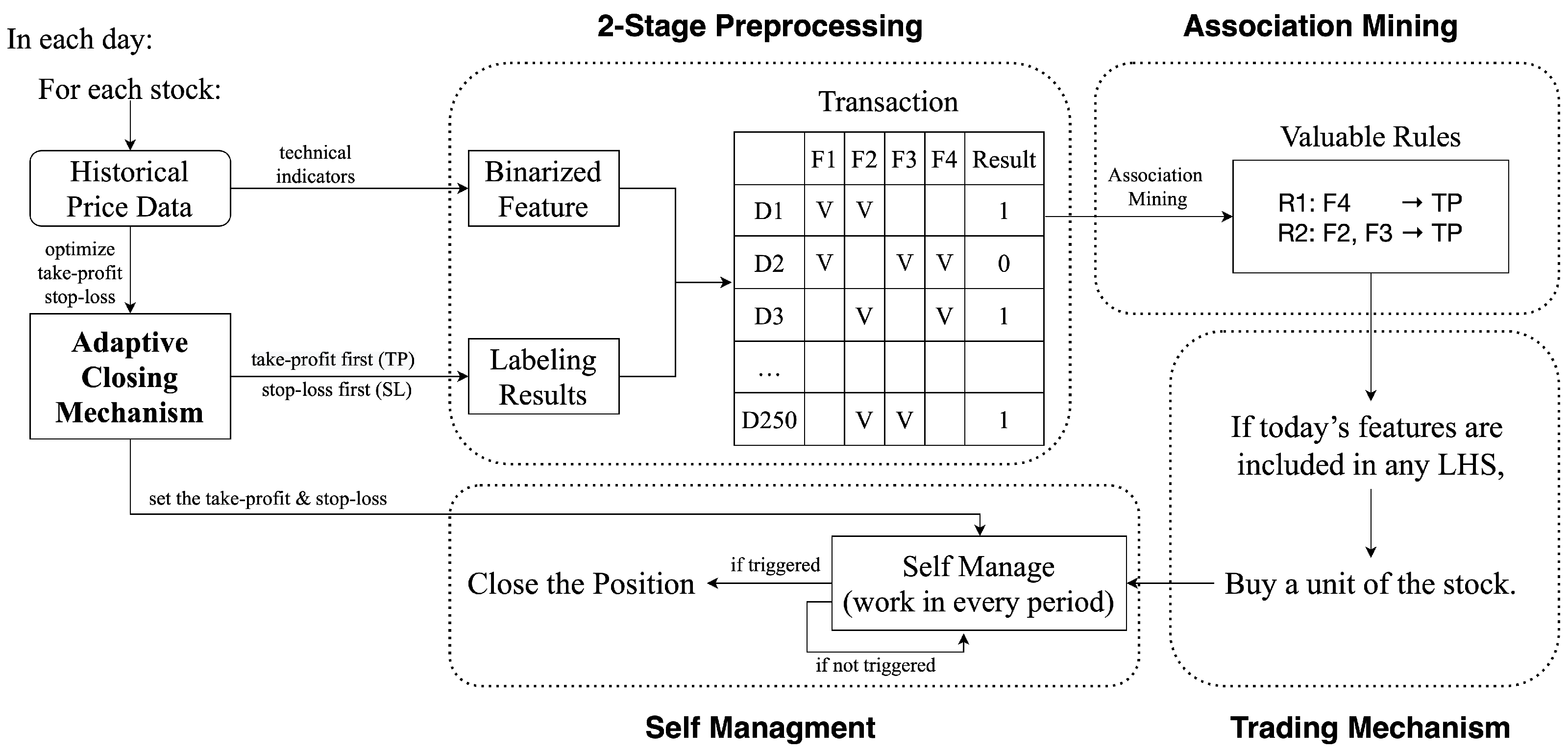
3. Proposed Self-Management Portfolio System

In this section, we demonstrate the proposed system, including five modules: trading mechanism, adaptive closing mechanism, self-management, two-stage preprocessing, and association mining modules. We first introduce the designed trading mechanism in Section 3.1, which is responsible for resource allocation. An adaptive closing mechanism is then presented to handle risk management (Section 3.2). Then, a self-management module is implemented to automatically manage trading positions, risks and resources (Section 3.3). After determining the trading and closing mechanism, a two-step preprocessing is performed to obtain the mining dataset (Section 3.4). Finally, an association mining module is presented in Section 3.5, which generates trading signals and acts as a decision-making module in the system.

Figure 1 shows the flowchart of the proposed system, and the designed modules are described in detail in the following subsections. In addition, an illustrative example as described in Section 3.6.

3.1. Trading Mechanism

3.1.1. Distributed Fund Unit

The trading mechanism is designed to only take the long position (buy first, then sell) and to be distributed and signal-driven. We divide the initial funds into M equal units, and detect the buying signals in each day (generated by association mining module in Section 3.5). For each buying signal, one fund unit is used to buy the stock that generated the signal. The distributed funds are designed to facilitate resource allocation and risk management (diversification).

Assuming that the initial capital (F) is divided into equal M units, then one fund unit (U) is:

$$\frac{F}{M}.$$

After the position is closed, the profits or losses are called the realized return, which will affect the number of fund units. In other words, if the system gets a positive cumulative realized return (generating profits), the system will have more fund units; vice versa, if the system gets a negative cumulative realized return (generating losses), the system will have fewer fund units. Let the cumulative realized return of day t be $CR{R}_t$, and let the number of total fund units of day t be $T{U}_t$. We then have:

$$T{U}_t=M+\lfloor \frac{CR{R}_t}{U}\rfloor ,$$

where $T{U}_t$ is a non-negative integer. Note that the cumulative realized return will not affect the size of a fund unit. As the number of total fund units increase, the system will have more units and more distributed investment (as a risk management).

Let the number of occupied fund units of day t be $O{U}_t$ (a positive integer), which means there are $O{U}_t$ units of funds in use (be used to buy stocks) of day t. If the $O{U}_t<T{U}_t$, the system still has free funds to trade of day t. Conversely, if $O{U}_t=T{U}_t$, the system has no free fund, and the system will turn into a sleep mode until the resource (funds) is released.

3.1.2. Details of Trading

Let $P_t$ be the stock price per share on day t, the rate of buying fee be $BFee$, and the rate of selling fee be $SFee$ (the fee includes commission, tax, and other cost). Suppose a stock generates a trading signal in day t, and the system has free fund unit to buy the stock. The system will buy one fund unit of the stock, and will obtain S shares, where the S is:

$$\lfloor \frac{U}{P_t\times (1+BFee)}\rfloor .$$

Suppose that the system decides to sell the stock on day $t^{\prime }$, the system can obtain:

$$S\times P_{t^{\prime }}\times (1-SFee).$$

Then, the realized return is:

$$S\times P_{t^{\prime }}\times (1-SFee)-S\times P_t\times (1+BFee).$$

The return rate of the trading is:

$$\frac{\mathrm{Realized}\mathrm{Return}}{S\times P_t\times (1+BFee)}=\frac{P_{t^{\prime }}\times (1-SFee)-P_t\times (1+BFee)}{P_t\times (1+BFee)}.$$

3.2. Adaptive Closing Mechanism

In the proposed system, we design an adaptive closing (selling) mechanism to handle the risk management and also discretize trading results (as items in the association mining). Two commonly-used closing mechanisms in financial trading are take-profit and stop-loss mechanisms [22,23].

3.2.1. Take-Profit and Stop-Loss Mechanisms

The take-profit mechanism indicates that once the unrealized return rate is higher than the take-profit threshold $TTP$ (a positive value), the position will be closed immediately. The stop-loss mechanism indicates that once the unrealized return rate is lower than the stop-loss threshold $TSL$ (a negative value), the position will be closed immediately. Assume a position is established (stock is bought) on day t at price $P_t$. If a take-profit mechanism with threshold of $TTP$ is implemented, the position will be closed on day $t+j$, where j is a positive integer satisfying:

$$\underset{j}{argmin}\frac{P_{t+j}\times (1-SFee)-P_t\times (1+BFee)}{P_t\times (1+BFee)}>TTP.$$

If a stop-loss mechanism with threshold of $TSL$ is implemented, the position will be closed on day $t+j$, where j is a positive integer satisfying:

$$\underset{j}{argmin}\frac{P_{t+j}\times (1-SFee)-P_t\times (1+BFee)}{P_t\times (1+BFee)}<TSL.$$

If a take-profit mechanism with $TTP$ and a stop-loss mechanism with $TSL$ are implemented at the same time, the position will be closed on day $t+j$, where j is a positive integer satisfying:

$$\begin{array}{cc}\hfill \underset{j}{argmin}& \hfill \frac{P_{t+j}\times (1-SFee)-P_t\times (1+BFee)}{P_t\times (1+BFee)}>TTP\vee \\ \hfill & \hfill \frac{P_{t+j}\times (1-SFee)-P_t\times (1+BFee)}{P_t\times (1+BFee)}<TSL.\end{array}$$

(1)

3.2.2. Adaptive Mechanisms

For each stock in each day, its characteristics may be different; therefore, the take-profit and stop-loss mechanism should adapt to its characteristics. The proposed adaptive closing mechanism dynamically adjusts $TTP$ and $TSL$ to adapt to the stock characteristics during each day. The mechanism utilizes historical data (the past 250 days, approximately the number of trading days in a year) to obtain the optimal take-profit and stop-loss thresholds, namely $OTTP$ and $OTSL$.

Let $R{R}_{t-j,t-1,TTP,TSL}$ be the return rate of stock bought on day $t-j$ with take-profit and stop-loss mechanisms (thresholds of $TTP$ and $TSL$), and closed at least on day $t-1$. Then, the optimal take-profit and stop-loss thresholds of the stock of day t, namely $OTT{P}_t$ and $OTS{L}_t$ are:

$$\underset{TTP,TSL}{argmax}\sum _{j=1}^{250}R{R}_{t-j,t-1,TTP,TSL},$$

(2)

where $TTP\in \{3\%,5\%,8\%,10\%,15\%,20\%\}$ and $TSL\in \{-3\%,-5\%,-8\%,-10\%\}$. Note that in the case of a smaller j, $t-j$ is close to $t-1$, which may cause the position bought on day $t-j$ haven’t been taken-profit or stopped-loss in day $t-1$. These positions should also be closed on day $t-1$, to avoid using the future information.

3.3. Self-Management

Association mining is the decision-making module in the proposed system, which generates trading (buying) signals. For each trading signal, the system will buy one fund unit of stock, and the position will be monitored by the self-management module, which monitors the adaptive closing mechanism and the existing time of the positions. For each position, both the take-profit and stop-loss mechanisms are applied with optimized thresholds. The self-management module will continuously monitor the stock price. Once the unrealized profits and losses are greater than the take-profit or stop-loss thresholds, the position will be closed immediately, as shown in Section 3.2.

Through preliminary experiments, we find that several positions occupy the funds for a long time, since the price fluctuates within a small range and does not reach the closing thresholds. Long-term occupied positions reduce the capital efficiency (opportunity cost, waste of other opportunities). Therefore, in order to better use of the resource, we design a timer to close the position if its existing time exceeds a threshold $Timer$. However, each position has different take-profit and stop-loss thresholds, and the $Timer$ for each position should be proportional to the distance of the threshold. For example, the timer of position with 10% take-profit and 10% stop-loss should be longer than the timer of position with 5% take-profit and 5% stop-loss, because the threshold distance is farther and must take longer time to be closed. We then design the timer $Timer$ to be:

$$Timer=round\left(\frac{(OTTP-OTSL)\times 400}{20}\right)\times 20,$$

where $round(·)$ denotes the nearest integer. In order to simplify the timer, we design the timer as multiples of 20 days (approximately the number of trading days in a month), and set the boundary of $Timer$ to $[20,120]$ to make it within a reasonable range (more than a month, less than a year), and $\in \{20,40,60,80,100,120\}$.

3.4. Two-Stage Preprocessing

To generate trading signals, the decision-making module in the proposed system is association mining, which searches for valuable associations (rules) between items. The rules ($X\Rightarrow Y$) can also be interpreted as features (X) guiding the interesting events (Y). In the financial trading, technical indicators are informative and representative features of stock market, and we use the indicators as items (features) for mining. We then define the interesting events as: when a stock is bought, the stock will take-profit first (before stop-loss) by the definition of adaptive closing mechanism in Section 3.2. Therefore, a two-stage preprocessing is designed; the first stage calculates technical indicators (features), and the second stage labels the interesting events.

In the first stage, we calculate several commonly-used technical indicators as the items (features) of association mining. We use relative strength index (RSI), stochastic oscillator (KD values), volume indicators, and also calculate the slope of closing price, average price, and volatility as additional features. RSI is a momentum indicator to measure the recent price changes [24]. KD values come from the stochastic oscillator to detect the overbought and oversold situation [25], where K-value (D-value) is for short-term (long-term) characteristic. In this paper, we utilize the K-value to obtain the long-term information. The volume indicator is defined as today’s trading volume divided by the average volume of previous 10 days. The slop features include the 10-day slop of the closing prices, average price, and price volatility. The average price and price volatility are the mean and variance of closing price in previous 10 days, which represent the trend of the price and volatility.

To simplify the calculation of feature and association mining, we discretize technical indicators into binary features. Since the RSI and K-value are continuous values in $[0,1]$, we discretize each value into four disjoint classes of $[0,0.25)$, $[0.25,0.50)$, $[0.50,0.75)$, and $[0.75,1)$. The volume indicator is also discretized into 4 disjoint classes of $[-\infty ,0.5)$, $[0.5,1)$, $[1,1.5)$, and $[1.5,\infty )$. For the slope features, we binarize the features by positive (include 0) and negative slopes. There are 18 $(=3\times 4+3\times 2)$ features in total. In the proposed system, users can replace technical indicators according to their own features, including news, trading volume, chip analysis and other information.

The second stage of preprocessing labels the interesting events. Since the adaptive closing mechanism applies different take-profit and stop-loss mechanisms in each day, we need to know whether the position is take-profit first or stop-loss first, as shown in Equation (1). In the case of take-profit first, the position generates profit, labeled as 1, and is the interesting event. In the case of stop-loss first, the position generates loss, labeled as −1. In the case that the position is forced to close on day $t-1$ (Equation (2)), the position may generate profit or loss, and is an uncertain situation, labeled as 0.

In order to improve the efficiency, lookup tables of features and labels can be established. Let Tab-Feature be the lookup table of stock features, where Tab-Feature($m,t$) is the features of m-th stock on t-th day, and is an 18-dimensional binary vector. Let Tab-Label be the lookup table of labels, where Tab-Label($m,t^{{}^{\prime }},t,OTT{P}_{m,t},OTS{L}_{m,t}$) is the label of the m-th stock bought on day $t^{{}^{\prime }}$ with take-profit and stop-loss mechanisms (thresholds of $OTT{P}_{m,t}$ and $OTS{L}_{m,t}$), and closed at least on day t, and is 1-dimensional with +1 for take-profit first, −1 for stop-loss first, and 0 for neither.

3.5. Association Mining

3.5.1. Transactions and Syntactic Constraint

When mine the rules of the m-th stock on the t-th day, let the optimized take-profit and stop-loss thresholds be $OTT{P}_{m,t}$ and $OTS{L}_{m,t}$, as defined in Section 3.2. To construct the transactions for mining, we concatenate the tables Tab-Feature($m,i$) and Tab-Label($m,i,t-1,OTT{P}_{m,t},OTS{L}_{m,t}$), where i is from $t-250$ to $t-1$, as defined in Section 3.4. The 250 transactions for the m-th stock on t-th day, called ${\mathbf{Tran}}_{m,t}$. Note that a Tab-Feature($m,i$) is a 18-dimensional Boolean vector, and a Tab-Label($m,i,t-1,OTT{P}_{m,t},OTS{L}_{m,t}$) is a label; therefore, a transaction is a 19-dimensional vector. An example for the transactions is shown in

Table 1. An example for the transactions.

F1	F2	F3	F4	⋯	F18	Label
1	0	1	1	⋯	1	+1
1	0	1	1	⋯	1	+1
1	1	0	0	⋯	1	−1
⋮	⋮	⋮	⋮	⋮	⋱	⋮
0	0	1	0	1	⋯	0

.

The designed association mining aims to find rules of features leading the +1 label. In the proposed system, the syntactic constraints are that the RHS only contains the +1 label and that the LHS only contains the features. For the m-th stock on t-th day, let the association mining find a rule of $X_{m,t}\Rightarrow +1$ through historical (250) transactions, where $X_{m,t}$ is a set of features that leads the +1 label. If the features of the m-th stock on $t-1$-th day (Tab-Feature($m,t$)) is a subset of $X_{m,t}$, the association module will generate a trading signal (buy the stock). Note that the association mining may find multiple rules, the trading signal will be triggered if any rules is fulfilled.

3.5.2. Confidence Constraint

For the confidence constraint, the system is only interested in profitable rules. A profitable rule should have sufficient confidence to make profitable decisions (positive expected return). Let the confidence level of a rule be $Conf$ and the optimized thresholds be $OTTP$ and $OTSL$, and let the total trading fee be $TFee$ (= $BFee+SFee$). The confidence is the true probability of the rule ($Conf$), which leads the +1 label, and obtains a return of $OTTP-TFee$. On the other hand, the false probability of the rule ($1-Conf$) does not lead the +1 label, and the worst case is obtaining a return of $OTSL-TFee$. Therefore, the expected return of the rule is:

$$Conf\times (OTTP-TFee)+(1-Conf)\times (OTSL-TFee).$$

We design a simple confidence constraint, which has at least a positive expected return (expected return $>0$), and the simple minimum confidence level is:

$$Conf>\frac{-OTSL+TFee}{OTTP-OTSL}.$$

(3)

We also design a strong confidence constraint to make the selected rules more profitable, which has at least a 3% expected return (expected return $>3$), and the strong minimum confidence level is:

$$Conf>\frac{3\%-OTSL+TFee}{OTTP-OTSL}.$$

(4)

3.5.3. Lift Constraint

The lift level is the conditional probability, $P\left(Y\right|X)$, divided by the probability $P\left(Y\right)$, as shown in Section 2.1. The lift constraint should be different to different stocks and days. For a stock with $P(Y=+1)$ of 0.1, it requires a large lift level to filter the large $P(Y=+1|X)$ (a representative rule). For stock with $P(Y=+1)$ of 0.9, it requires a small lift level to keep the rules. If the minimum lift is set to 1.2, the $P(Y=+1|X)$ should be larger than 1.8 ($0.9\times 2$), which is impossible and left no rule.

In order to dynamically adjust the lift, we utilize the historical data (validation set and rolling window are used) to select the lifts for each stock in each day, as shown in Figure 2.

To select the lift for the m-th stock on t-th day ($Lif{t}_{m,t}$), we utilize the ${\mathbf{Tran}}_{m,t-100}$ to ${\mathbf{Tran}}_{m,t-1}$ as the validation to select the lift. Let the optimized take-profit and stop-loss thresholds be $OTT{P}_{m,t}$ and $OTS{L}_{m,t}$. The $Lif{t}_{m,t}$ is defined to optimize the trading return on the day of $t-100$ to $t-1$ (validation set), and is defined as:

$$\underset{lift}{argmax}\sum _{j=1}^{100}ARe{t}_{t-j,t-1,OTT{P}_{m,t},OTS{L}_{m,t}}({\mathbf{Tran}}_{m,t-j},\mathbf{Tab}-\mathbf{Feature}(m,t-j),lift),$$

where $lift$ is in $\{1.0,1.5,2.0,3.0,4.0\}$. The $ARet$ is the return rate of the association rule trading (mine ${\mathbf{Tran}}_{m,t-j}$ with a lift constraint of $lift$, and buy the m-th stock on $(t-j)$-th day if $\mathbf{Tab}-\mathbf{Feature}(m,t-j)$ is a subset of any mined rules, as described in Section 3.5.1). Note that the position is with take-profit and stop-loss mechanisms, and the thresholds are constant to $OTT{P}_{m,t}$ and $OTS{L}_{m,t}$ (not change from $t-250$ to $t-1$, since the system aims to find the lift for the t-th day with that thresholds). Additionally, note that the position will force to close at least on day $t-1$ to prevent using future information.

3.6. Illustrative Example

We divide the funds into M units, and trade and manage each unit separately. In each trading day, for each stock, we use historical data to select optimized take-profit threshold, stop-loss threshold, and lift. Then, the features and labels of the previous 250 days are calculated to form the mining dataset. After mining valuable rules, if today’s features are a subset of any rules, buy a unit of stock. The self-management module will then monitor the stop-loss and take-profit mechanism and timer. Not that since we perform the system on daily opening, highest, lowest, closing price (OHLC) data (low frequency, is difficult to trade in real time), we buy the stock on next trading day (at closing price) and sell the stock on next trading day (at opening price) to increase the liquidity and scalability of the system and to make the system be tradable in the real-world market.

4. Experimental Results and Discussion

In this section, we first investigate the system performance with different modules, as shown in Section 4.1. A comparison between the system and benchmarks is then presented in Section 4.2.

In this paper, we implemented the proposed system on the Taiwan stock market from 30 June 2003 to 31 December 2019. The stock pool contained the constituent stocks of Taiwan-50 and Mid-Cap-100, which were the top 150 (=50 + 100) stocks that had the largest capital value on Taiwan stock market. For each trading signal, we bought stocks at tomorrow’s closing price and sold stocks at tomorrow’s opening price. Since the stocks had high liquidity, we assumed that there was no slippage in the tradings. The buying and selling fees ($BFee$ and $SFee$) were set to 0.001425 and 0.004425, which included all the fees and taxes charged by the Taiwan stock market.

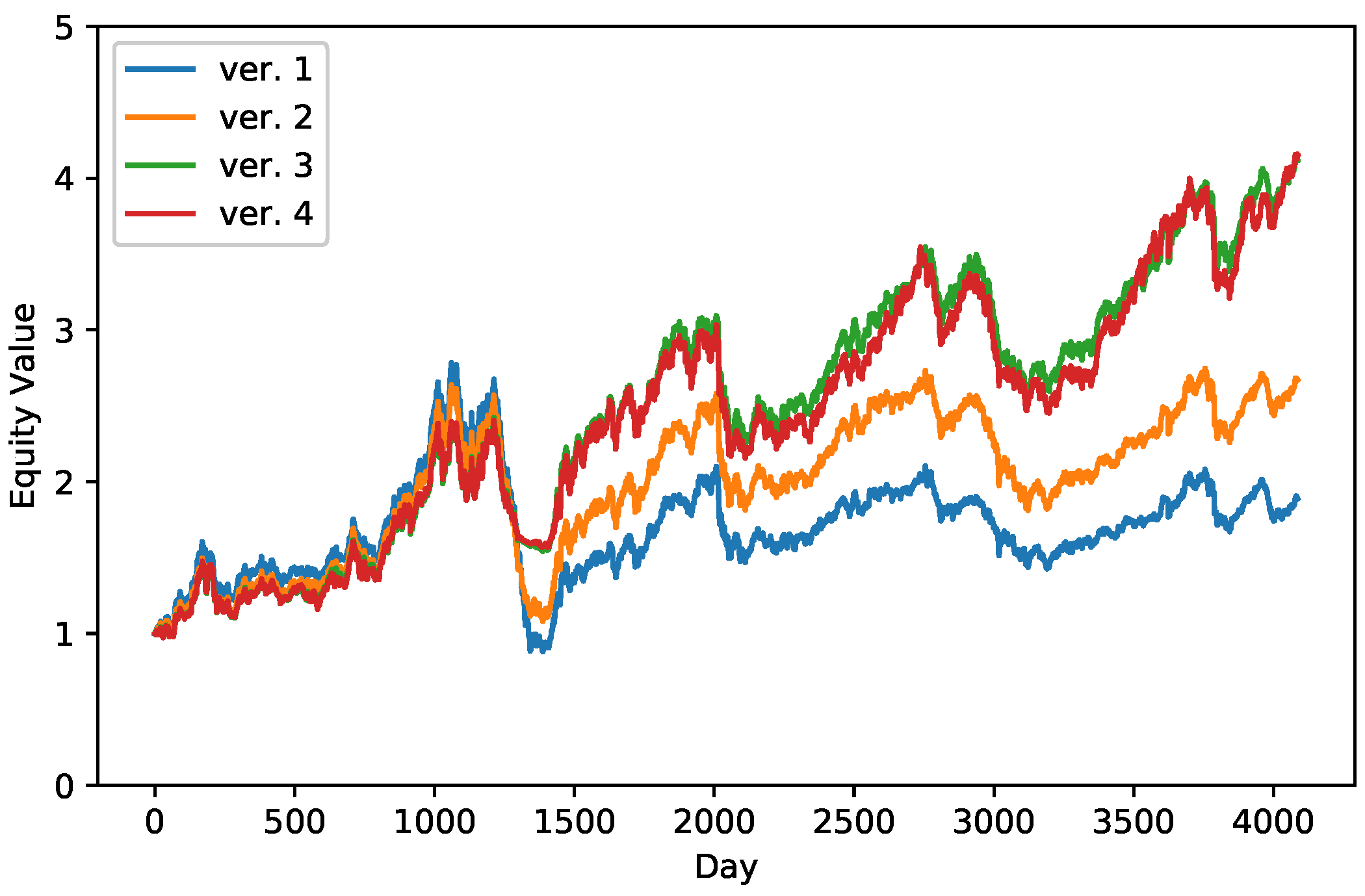
4.1. System Performance with Different Modules

In this section, we demonstrate the trading performance of systems with different modules, named them from ver. 1 to ver. 4. As the version number increased, more modules were stacked on, as shown in

Table 2. Performance indicators of the proposed systems.

Systems	ver. 1	ver. 2	ver. 3	ver. 4
Confidence	Simple	Strong	Strong	Strong
Lift	No	No	Dynamic	Dynamic
Timer	No	No	No	Dynamic
Annual Return	4.0%	6.2%	9.0%	9.1%
Sharpe Ratio	0.233	0.379	0.600	0.578
MDD	68.4%	59.0%	36.3%	34.6%

. The first system (ver. 1) was a pure system that only obtained simple confidence constraint, as defined in Equation (3) (no lift constraint and timer). The second system (ver. 2) enhanced the confidence level to the strong confidence constraint, as defined in Equation (4). The simple and strong confidence constraints are described in Section 3.5.2. The third system (ver. 3) added the dynamic lift constraint, as described in Section 3.5.3. The fourth system (ver. 4) added the timer in the self-management module, as shown in Section 3.3.

The trading results (performance indicators) of each system are listed in Table 2. It can be found that the trading performance improved as more modules were adopted in the system, especially the dynamic lift module. The module of dynamics lift (from ver. 2 to ver. 3) significantly improved the annual return rate and the Sharpe ratio (increased 2.8% and 0.221), and sharply reduced the drawdown risk (decreased 22.7%). The ver. 4 system finally boosted the annual return and Sharpe ratio to 9.1% and 0.578, which were 2.28 and 2.48 times that of ver. 1, respectively. At the same time, the ver. 4 system dramatically reduced the drawdown risk to 34.6%, which was almost half of that of ver. 1.

Figure 3 shows the equity curves of the proposed systems (ver. 1 to ver. 4). The x-axis is the index of day. The left and right y-axes are the equity and the stock values, where the equity value is the sum of the stock and cash values. The curves are the equity values, which corresponds to the left y-axis. The bars under the curves are the stock value at each time (corresponds to the right y-axis), and the bars are always below the curves since there was no negative cash value. In other words, the height from the top of the bar (stock value) to the curve (equity value) is the cash value (white area). The bars represent the capital utilization, and the higher bar represents higher capital utilization (more stock positions and less cash).

Encouragingly, in the severe bear markets (downward market trends), the proposed systems rapidly closed the stock positions to avoid drawdown risk and gradually increased the stock positions to pursue growing profits when the market turned into a bull market (upward market trend), especially the ver. 3 and ver. 4 in Figure 3c,d. This phenomenon could be observed in the periods of 1200–1400 days (financial crisis of 2007 to 2008) and 3700–4000 days (China–United States trade war from 2018), and showed the efficacy of risk management of the proposed system. We overlapped the equity curves of ver. 1 to ver. 4 in Figure 4. It can also be found that the trading performance improved as more modules were adopted in the system (from ver. 1 to ver. 4), and the cumulated equities were getting higher and higher.

4.2. Comparison between Benchmarks

In this paper, we used two competitive passive investment strategies and Paranjape-Voditel and Umesh’s system [13] (state-of-art trading system based on association mining) as benchmarks. Two passive investment strategies were equal-weight [26] (1/N portfolio) and value-weight [27] (portfolio weighted by market capitalization). We use Taiwan-50 exchange traded fund (ETF) as the value-weighted type benchmark, which is the largest and most popular ETF on the Taiwan stock market. For the Paranjape-Voditel and Umesh’s system, we reproduced their system without the fuzzy logic and time lags (which had better performance). We divided the 150 stocks into 10 sectors, and bought the top-three stocks in the top-two sectors with a 1-year rebalancing day, as the setting in [13].

Table 3. Performance indicators of the proposed system and benchmarks.

Systems	Annual Return	Sharpe Ratio	MDD
Proposed System-ver. 4	9.1%	0.578	34.6%
Proposed System-ver. 3	9.0%	0.600	36.3%
Equal Weight	6.8%	0.431	55.1%
Taiwan-50 ETF (0050.TW)	7.3%	0.369	59.0%
Paranjape-Voditel and Umesh [13]	5.5%	0.235	69.0%

lists the performance indicators of the proposed systems and benchmarks, and the values shown in bold are the best ones among all strategies. In the table, the proposed systems (ver. 3 and ver. 4) outperformed all benchmarks in all aspects (profitability and risk measurements). Figure 5 presents the net equity curves of the strategies. It could be found that the equity curve of the proposed system suppressed the curves of benchmarks after 1200-th day. Furthermore, the proposed system obtained relatively slight drawdown in the severe bear markets, including the financial crisis of 2007 to 2008 (1200–1400 days) and China–United States trade war from 2018 (3700–4000 days). Overall, the outstanding performance showed the well-managed resources and trading risks of the proposed system.

4.3. Robustness Analysis on Random Stock Pools

In order to analyze the robustness of the proposed system, we randomly sampled the stock pool of the system and evaluated the performance. We randomly selected 50 stocks from 150 stocks (Taiwan 50 and Mid-Cap 100) to form a stock pool and implement in the system. The sampling was repeated three times (named as RS1, RS2, and RS3), and the performance indicators of each stock pool are listed in

Table 4. Performance indicators of the proposed system on different stock pools.

Systems	Annual Return	Sharpe Ratio	MDD
All stocks-ver. 3	9.0%	0.600	36.3%
All stocks-ver. 4	9.1%	0.578	34.6%
RS1-ver. 3	8.3%	0.588	27.8%
RS1-ver. 4	8.1%	0.562	32.8%
RS2-ver. 3	8.9%	0.636	26.0%
RS2-ver. 4	8.5%	0.604	29.1%
RS3-ver. 3	9.5%	0.678	26.1%
RS3-ver. 4	8.7%	0.619	26.4%

.

The annual returns of RS1 to RS3 were slightly lower than that of all stocks, which may be due to fewer stocks to choose (reduced from 150 to 50). However, the Sharpe ratios still maintained high quality, even reaching a new high of 0.678. Surprisingly, the MDDs were further decreased to a new low of 26.0%. To sum up, the proposed systems still had outstanding performance on randomly sampled stock pools, which also outperformed the benchmarks and further reduce trading risks. The experiment showed the robustness and sustainability of the system.

5. Conclusions

A well-established financial trading system should well perform in resource allocation, risk management, and sustainability. The quality of resource allocation critically affects the performance; however, when pursuing outstanding profits, trading risk will be simultaneously raised. Therefore, risk management and sustainability are crucial issues for investment. With the rapid development of data mining, association mining, is an efficient, intuitive and interpretable tool, and is also an ideal algorithm for financial decision-making. In this paper, we propose a self-management portfolio system with adaptive association mining for practical applications. The system allocates funds into independent units to well manage the trading risks, and utilizes association mining as a resource allocation module, and adopts adaptive closing mechanism to achieve sustainability, and employs a self-management module to continuously monitor the holding positions. Experimental results show that proposed system boosts the annual return and Sharpe ratio to 9.1% and 0.578 (increased to 2.28 and 2.48 times), and reduces the drawdown risk to 34.6% (decreased to almost half). Furthermore, in the bear markets, the systems rapidly close the stock positions to avoid drawdown risk and gradually increase the stock positions to pursue growing profits when the market turns into bull market. Compared with benchmarks, proposed system outperforms all benchmarks in all measurements, where randomly sampled datasets are also included. For the future work, we will extend the system to other commodities that are not limited to stocks.

References

1. Wu, M.E.; Syu, J.H.; Lin, J.C.W.; Ho, J.M. Portfolio management system in equity market neutral using reinforcement learning. Appl. Intell. 2021, 1–13. [Google Scholar] [CrossRef]
2. Amit, R.; Livnat, J. Diversification and the risk-return trade-off. Acad. Manag. J. 1988, 31, 154–166. [Google Scholar] [CrossRef]
3. Chong, Y.Y. Investment Risk Management; John Wiley & Sons: Hoboken, NJ, USA, 2004. [Google Scholar]
4. Koellner, T.; Weber, O.; Fenchel, M.; Scholz, R. Principles for sustainability rating of investment funds. Bus. Strat. Environ. 2005, 14, 54–70. [Google Scholar] [CrossRef]
5. Giudici, P.; Figini, S. Applied Data Mining for Business and Industry; Wiley Online Library: Hoboken, NJ, USA, 2009. [Google Scholar]
6. Berry, M.J.; Linoff, G.S. Data Mining Techniques: For Marketing, Sales, and Customer Relationship Management; John Wiley & Sons: Hoboken, NJ, USA, 2004. [Google Scholar]
7. Kovalerchuk, B.; Vityaev, E. Data Mining in Finance: Advances in Relational and Hybrid Methods; Springer Science & Business Media: New York, NY, USA, 2006; Volume 547. [Google Scholar]
8. Grossman, R.L.; Kamath, C.; Kegelmeyer, P.; Kumar, V.; Namburu, R. Data Mining for Scientific and Engineering Applications; Springer Science & Business Media: New York, NY, USA, 2013; Volume 2. [Google Scholar]
9. Tsai, C.W.; Lai, C.F.; Chiang, M.C.; Yang, L.T. Data mining for internet of things: A survey. IEEE Commun. Surv. Tutor. 2013, 16, 77–97. [Google Scholar] [CrossRef]
10. Syu, J.H.; Wu, M.E.; Srivastava, G.; Chao, C.F.; Lin, J.C.W. An IoT-based Hedge System for Solar Power Generation. IEEE Int. Things J. 2021. [Google Scholar] [CrossRef]
11. Lu, H.; Han, J.; Feng, L. Stock movement prediction and n-dimensional inter-transaction association rules. In Proceedings of the 1998 ACM SIGMOD Workshop on Research Issues on Data Mining and Knowledge Discovery, Seattle, WA, USA, 5 June 1998; ACM: New York, NY, USA, 1998. [Google Scholar]
12. Liao, S.H.; Ho, H.H.; Lin, H.W. Mining stock category association and cluster on Taiwan stock market. Exp. Syst. Appl. 2008, 35, 19–29. [Google Scholar] [CrossRef]
13. Paranjape-Voditel, P.; Deshpande, U. A stock market portfolio recommender system based on association rule mining. Appl. Soft Comput. 2013, 13, 1055–1063. [Google Scholar] [CrossRef]
14. Agrawal, R.; Imieliński, T.; Swami, A. Mining association rules between sets of items in large databases. In Proceedings of the 1993 ACM SIGMOD International Conference on Management of Data, Washington, DC, USA, 26–28 May 1993; pp. 207–216. [Google Scholar]
15. Lin, W.; Alvarez, S.A.; Ruiz, C. Efficient adaptive-support association rule mining for recommender systems. Data Mining Knowl. Discov. 2002, 6, 83–105. [Google Scholar] [CrossRef]
16. Na, S.H.; Sohn, S.Y. Forecasting changes in Korea composite stock price index (KOSPI) using association rules. Exp. Syst. Appl. 2011, 38, 9046–9049. [Google Scholar] [CrossRef]
17. Uyemura, D.G.; Kantor, C.C.; Pettit, J.M. EVA® for banks: Value creation, risk management, and profitability measurement. J. Appl. Corp. Financ. 1996, 9, 94–109. [Google Scholar] [CrossRef]
18. Chen, J. Annual Return. 2019. Available online: http://investopedia.com/ (accessed on 15 April 2021).
19. Magdon-Ismail, M.; Atiya, A.F. Maximum drawdown. Risk Mag. 2004, 17, 99–102. [Google Scholar]
20. Sharpe, W.F. The Sharpe ratio. J. Portf. Manag. 1994, 21, 49–58. [Google Scholar] [CrossRef]
21. Bailey, D.H.; Prado, M.L.d. The Sharpe ratio efficient frontier. J. Risk 2012, 15, 13. [Google Scholar] [CrossRef] [Green Version]
22. Wu, M.E.; Syu, J.H.; Lin, J.C.W.; Ho, J.M. Evolutionary ORB-based model with protective closing strategies. Knowl. Based Syst. 2021, 216, 106769. [Google Scholar] [CrossRef]
23. Syu, J.H.; Wu, M.E. Modifying ORB trading strategies using particle swarm optimization and multi-objective optimization. J. Ambient Intell. Humaniz. Comput. 2021, 1–13. [Google Scholar] [CrossRef]
24. Taran Morosan, A. The relative strength index revisited. Afr. J. Bus. Manag. 2011, 5, 5855. [Google Scholar]
25. Stochastic Oscillator. Available online: https://school.stockcharts.com/doku.php?id=technical_indicators:stochastic_oscillator_fast_slow_and_full (accessed on 15 April 2021).
26. DeMiguel, V.; Garlappi, L.; Uppal, R. Optimal versus naive diversification: How inefficient is the 1/N portfolio strategy? Rev. Financ. Stud. 2009, 22, 1915–1953. [Google Scholar] [CrossRef] [Green Version]
27. Plyakha, Y.; Uppal, R.; Vilkov, G. Equal or value weighting? Implications for asset-pricing tests. Implic. Asset-Pricing Tests 2014. [Google Scholar] [CrossRef]
Figure 1. The flowchart of the proposed system.
Mathematics 09 01093 g001
Figure 2. The schematic diagram of dynamic lift.
Mathematics 09 01093 g002
Figure 3. Trading performance of the proposed systems.
Mathematics 09 01093 g003
Figure 4. Equity curves of the proposed systems.
Mathematics 09 01093 g004
Figure 5. Equity curves of the proposed system and benchmarks.
Mathematics 09 01093 g005