Article

An Improved Machine Learning-Based Employees Attrition Prediction Framework with Emphasis on Feature Selection

by
Saeed Najafi-Zangeneh
1,
Naser Shams-Gharneh
1,
Ali Arjomandi-Nezhad
2 and
Sarfaraz Hashemkhani Zolfani
3,*
1
Industrial Engineering Department, Amirkabir University of Technology, Tehran 15875-4413, Iran
2
Industrial Engineering and Productivity Research Center, Amirkabir University of Technology, Tehran 15875-4413, Iran
3
School of Engineering, Catholic University of the North, Larrondo 1281, 1780000 Coquimbo, Chile
*
Author to whom correspondence should be addressed.
Mathematics 2021, 9(11), 1226; https://doi.org/10.3390/math9111226
Submission received: 26 April 2021 / Revised: 26 May 2021 / Accepted: 26 May 2021 / Published: 27 May 2021
(This article belongs to the Special Issue Multi-Criteria Decision Making and Data Mining)

Abstract

:
Companies always seek ways to make their professional employees stay with them to reduce extra recruiting and training costs. Predicting whether a particular employee may leave or not will help the company to make preventive decisions. Unlike physical systems, human resource problems cannot be described by a scientific-analytical formula. Therefore, machine learning approaches are the best tools for this aim. This paper presents a three-stage (pre-processing, processing, post-processing) framework for attrition prediction. An IBM HR dataset is chosen as the case study. Since there are several features in the dataset, the “max-out” feature selection method is proposed for dimension reduction in the pre-processing stage. This method is implemented for the IBM HR dataset. The coefficient of each feature in the logistic regression model shows the importance of the feature in attrition prediction. The results show improvement in the F1-score performance measure due to the “max-out” feature selection method. Finally, the validity of parameters is checked by training the model for multiple bootstrap datasets. Then, the average and standard deviation of parameters are analyzed to check the confidence value of the model’s parameters and their stability. The small standard deviation of parameters indicates that the model is stable and is more likely to generalize well.

1. Introduction

Human resource is the initial source and the most critical essence of each company. Managers spend a considerable amount of time recruiting capable employees. Furthermore, they regularly spend additional resources on training staff. Every employee attrition, quitting the job without replacement, imposes a cost on the company for recruiting and training a new employee. To illustrate the definition of attrition, consider two cases (a) and (b). In case (a), which is not attrition, the employer decides to replace an employee with another more skilled person. In case (b), which is attrition, an employee leaves the company. Obviously, in the second case, the employer faces delays in its project schedule, due to recruiting and training the replacement employee. Predicting attrition makes it easier for decision-makers to take proper preventive actions. Several factors, such as age, salary, distance from home, education level, etc., contribute to whether an employee decides to leave a company or not. Since there is no deterministic analytical relation between employee attrition and these influential factors, machine learning approaches, which are computational methods that use experience to improve performance or make accurate predictions [1], can be utilized.
Several works in the literature aim at building a classifier to predict if a particular employee leaves. Mohbey and Kumar in [2] trained Random Forest, Naïve Bayes, Logistic Regression, SVM, and Decision Tree classifiers for this task. The precision, recall, and F1-score values reveal that Logistic Regression performed well in the attrition prediction task, and some indicators of this model are higher than those of other classifiers. A Logistic Regression classifier is employed in [3] for the IBM HR database employee attrition prediction. However, this paper did not select influential features. The database consists of a number of features. Only eight employees from 70 predicted attritions really quit their jobs. The other 62 samples were wrongly predicted as attritions. Reference [4] trained Logistic Regression, Random Forest, and K-Nearest Neighbor (KNN) models for attrition prediction. This paper used Principal Component Analysis (PCA) to reduce the feature space’s dimensionality.
Nevertheless, many features in attrition databases are binary variables for which the PCA algorithm does not work well. Besides, PCA reduces the dimension based on the linear relationship between features. It does not investigate the potential relation between candidate features and output. The authors of [5] first eliminated those variables which weakly correlate with other variables. Then, a feature selection based on random forest was performed. At last, a Logistic Regression model for attrition prediction was trained.
Papers [3,4,5] did not evaluate recall and precision measures, which are necessary for performance analysis in case of significant dataset imbalance. On the other hand, many papers computed these measures and aimed at increasing them. The authors of [6] resampled the dataset to make it balanced and increase the predictor’s performance. They resampled the dataset before separating the training and test sets. Although we adhere to their claim about enhancing performance due to resampling, resampling before training and test set separation would lead to a misunderstanding of the model’s performance. Some training samples may repeat themselves in the test dataset by resampling before separating the training and test datasets. The model would perform well for these particular test samples. Thus, the generalization capacity of the model may be overestimated. Some linear models, including linear regression and Linear Discriminant Analysis, are used in [7] in order to predict whether an employee intends to leave. The paper computed recall and precision measures based on the class of employees who stayed with the company. This class is more populated, and thereby the performance of the classifier is over-estimated. Classifiers are usually more precise at predicting the populated class. The principal challenge is to predict the minority class precisely. An Artificial Neural Network (ANN) attrition predictor was presented in [8]. Despite the great achievements of this paper, the performance of the model was examined using mean square error and accuracy. Mean square error is not a good performance indicator for classification tasks, and accuracy is not sufficient for performance analysis of imbalanced datasets. Authors in [9] tried several classifiers, including logistic regression, AdaBoost, random forest, and gradient boosting for attrition prediction. Although this work is comprehensive, the recall and precision of these models are not compared. Besides, it used the correlation-based feature selection, which could not result in a good selection of the most influential features. The relationship between the features is visualized in [10]. This accommodation provides a decent perception of the dataset. Then, several classifiers are trained for attrition prediction on the IBM HR dataset. The F1-score measures were not satisfactory values. Reference [11] modeled some attrition predictors and presented an analysis of which departments employees are more likely to leave.
Each paper in the existing literature is lacking in one or some of the following aspects:
  • Proper feature selection method
  • Informative evaluation of the classifier’s performance
  • Confidence levels for the value of the coefficient of each feature in the logistic regression model
A proper study of attrition prediction tasks should include pre-processing, processing, and post-processing stages in order to present a practical, reliable predictor that human resource managers can trust. At the pre-processing stage, features that are most relevant to this task are selected. Besides, redundant features are eliminated. A proper feature selection enhances the performance of the models that are trained at the processing stage. At the processing stage, the predictor model is trained, tested, and compared with other models. Finally, how much confidence in the model at the post-processing stage must be ensured.
To the best of our knowledge, this paper, for the first time, proposes an attrition prediction task that addresses all three stages of pre-processing, process, and post-processing. First of all, the “max-out” algorithm, which is a novel feature selection method for enhancing the performance of our attrition prediction classifier, is presented as the pre-processing stage. Then, a logistic regression model is trained for the new set of features for the processing stage. Next, confidence analysis for quantifying how sure we are about our model’s parameters is introduced at the post-processing stage. Finally, the methodology is verified using IBM attrition data [12]. The general structure of the proposed framework is shown in Figure 1. In this figure, yellow, green, and red blocks depict pre-processing, processing, and post-processing stages. The main objective of these steps is to make sure that the model is able to generalize properly.
The rest of this paper is organized as follows. Section 2 introduces the “max-out” method and discusses the complexity of the algorithm. Next, the parameters’ confidence analysis is introduced in Section 3. Then, logistic regression, which is the predictor of attrition, is briefly reviewed in Section 4. After that, Section 5 studies this algorithm’s capability to enhance the IBM attrition classifier’s performance. Finally, conclusions are drawn in Section 6.

2. Feature Selection

Several unnecessary features can be eliminated in the pre-processing stage. One solution is to train the model for every subset of features and then compare the validation dataset metrics. This procedure requires 2n times training the model for a dataset with n features. Thus, it is highly time-consuming. Several feature selection methods have been previously presented for this particular procedure as summarized in Table 1 [13,14]. Filter methods are based on the correlation between the values of features.
On the other hand, wrapper methods concentrate on selection based on the classifier’s performance with the selected features. Embedded methods embed feature selection in the learning algorithm. Hybrid methods are those which are a combination of these methods. A comparison between these categories is provided in Table 1 [13,14]. Notice that the feature selection method should be consistent with the nature of the features.

2.1. Max-Out Feature Selection Algorithm

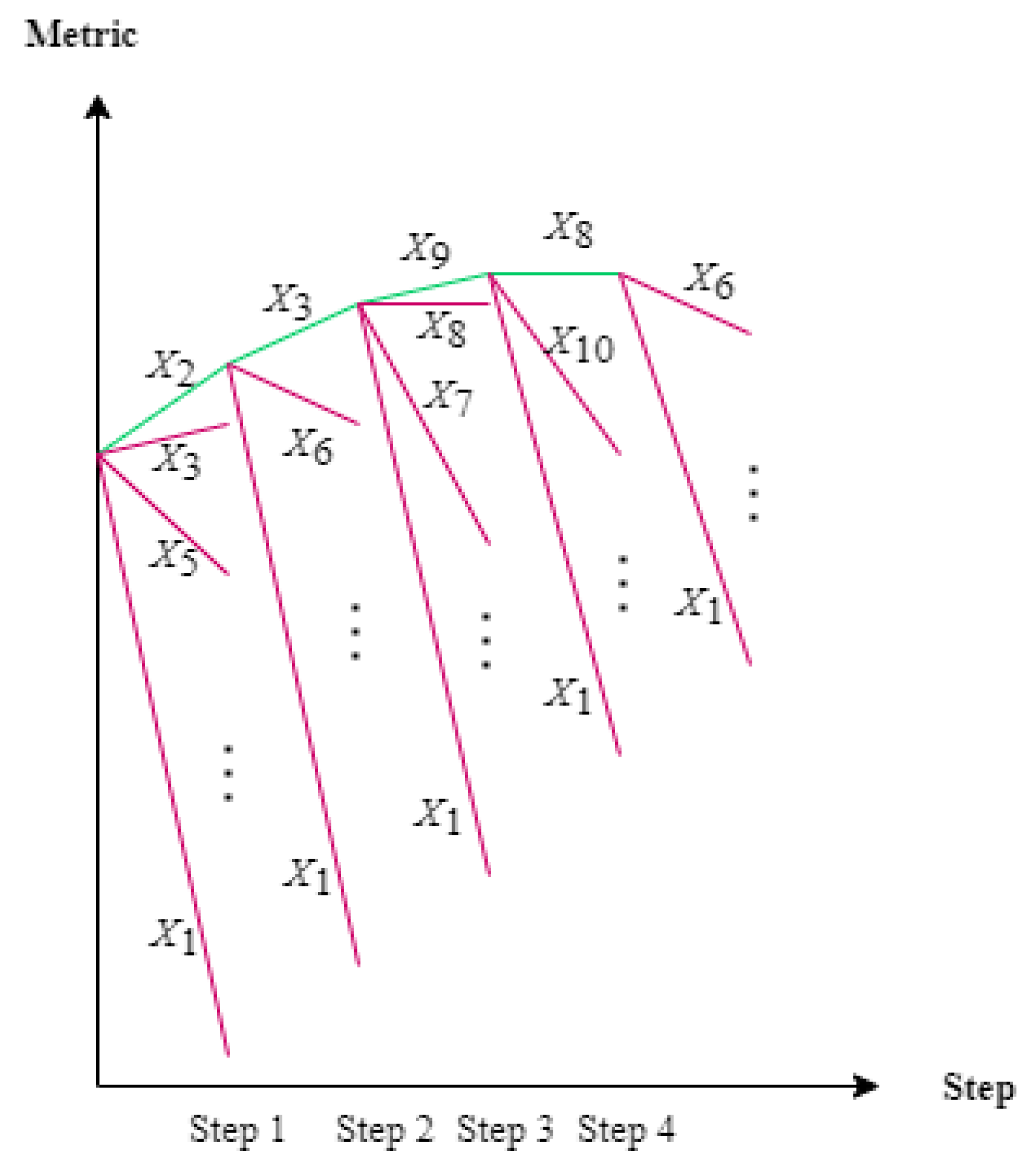
Based on the nature of this problem’s feature set, which includes both binary and continuous features, the “max-out” algorithm feature selection, which belongs to the wrapping category, is developed. The algorithm is expressed in Algorithm 1. According to this algorithm, firstly, all subsets of n-m features are trained. The subset with the most significant metric is chosen as the feature set. The process is repeated for the new set of features. When the metric gets smaller than the previous step, the feature set is not changed further. Since the model is trained for only a portion of all possible features, the algorithm is much faster than checking all possible combinations of features. If m is equal to 1, the algorithm is called 1-max-out, and if m is 2, the algorithm is called 2-max-out. The 1-max-out algorithm is backward feature selection [22]. However, in some special cases, the inclusion of m features together may enhance the performance. Still, every one of them may not have a significant role in the classification performance. Therefore, 1-max-out may wrongly eliminate these features one after another. In these cases, m-max-out (m > 1) performs better than 1-max-out. The m-max-out is of the order of O(fm), given f as the number of initial features. Therefore, choosing a suitable m is also dependent on the available computation resources.
Figure 2 provides an example in which omitting four (X2, X3, X9, X8) features from the total fifteen is the best feature selection determined by the “1-max-out” method. This process takes 14 iterations to identify the first feature, which should be omitted, 13 iterations for the second, 12 iterations for the third, 11 iterations for the fourth, and 10 iterations for realizing that further eliminations do not help. If we wanted to perform a brute-force search, 215, which is equal to 32,768, times training the model, is required.
Algorithm 1 m-max-out
  • Create SetF = Set of all n features.
  • Compute variable M as the metric of a classifier with features of SetF
  • Take n equal to the size of SetF
  • Create Sub1, Sub2, …, Subk all subsets of size n-m of SetF.
  • Compute the metric for Sub1, …, Subk.
  • Take M’ equal to the biggest metrics’ value of sets of line 4 (for the corresponding subset j).
  • If M’ ≥ M: M=M’ and SetF=Subj and go to 3

2.2. Illustrative 1-Max-out Example

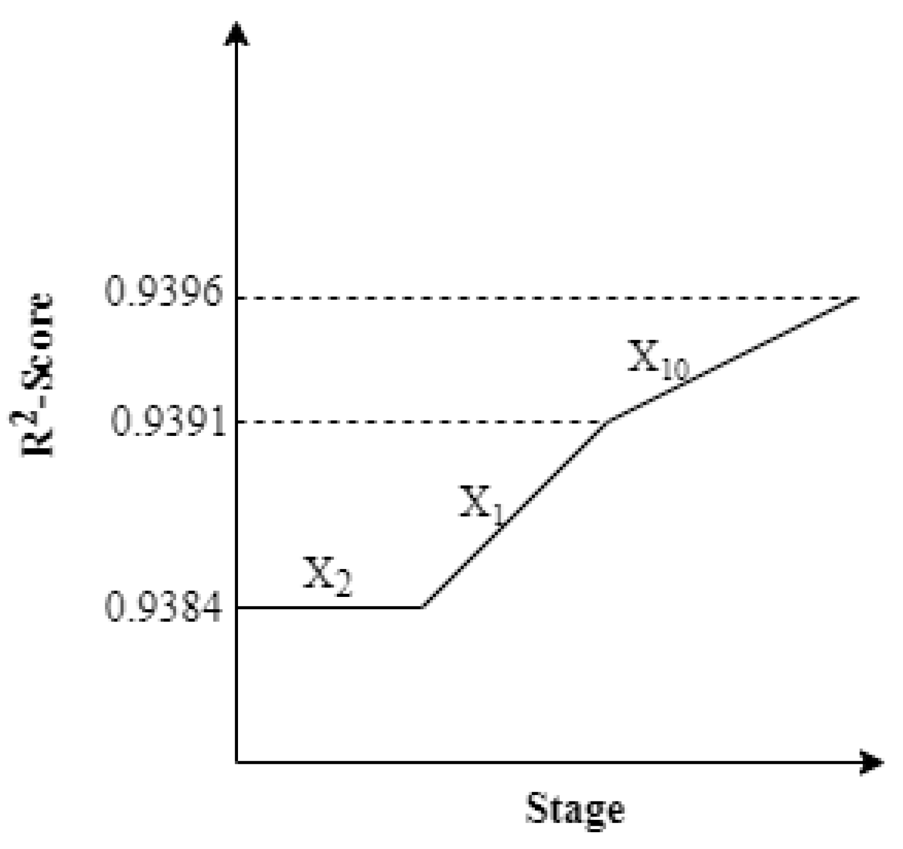
In order to further illustrate the Max-Out method, an example of the fish market problem [23] is discussed in this section. Notice that this is not the main case study of this paper. The objective of this benchmark problem is to predict the weight of fish. There are seven binary variables, “Bream”, “Parkki”, “Perch”, “Pike”, “Roach”, “Smelt”, “Whitefish” and five continuous variables, “Length1”, “Length2”, ”Length3”, and “Height”, “Width.” After indexing these from 0 to 11, the 1-max-out algorithm is performed. As Figure 3 depicts, the variables 2, 1, and 10 are removed in succession. As a result of this feature selection, the R2-score measure for the validation set increases from 0.9384 to 0.9396, and for the test set from 0.9145 to 0.9179.

3. Parameter Confidence Analysis

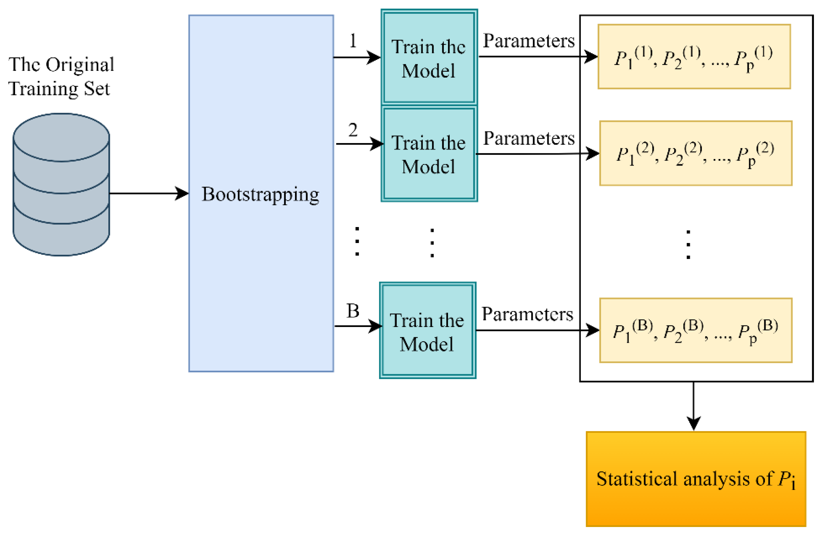
In order to check how much we are confident about the value of the parameters of our model, the procedure in Figure 4 is performed. Each time we produce a new dataset by bootstrapping (resampling by replacement [24]) the primary training dataset, our model changes its parameters. If the model overfits the training set, the variation of parameters would be significant. Otherwise, parameters vary slightly, which means that the parameters estimate the real trend, not just memorizing the training set. Various statistical analyses can be performed on each parameter.
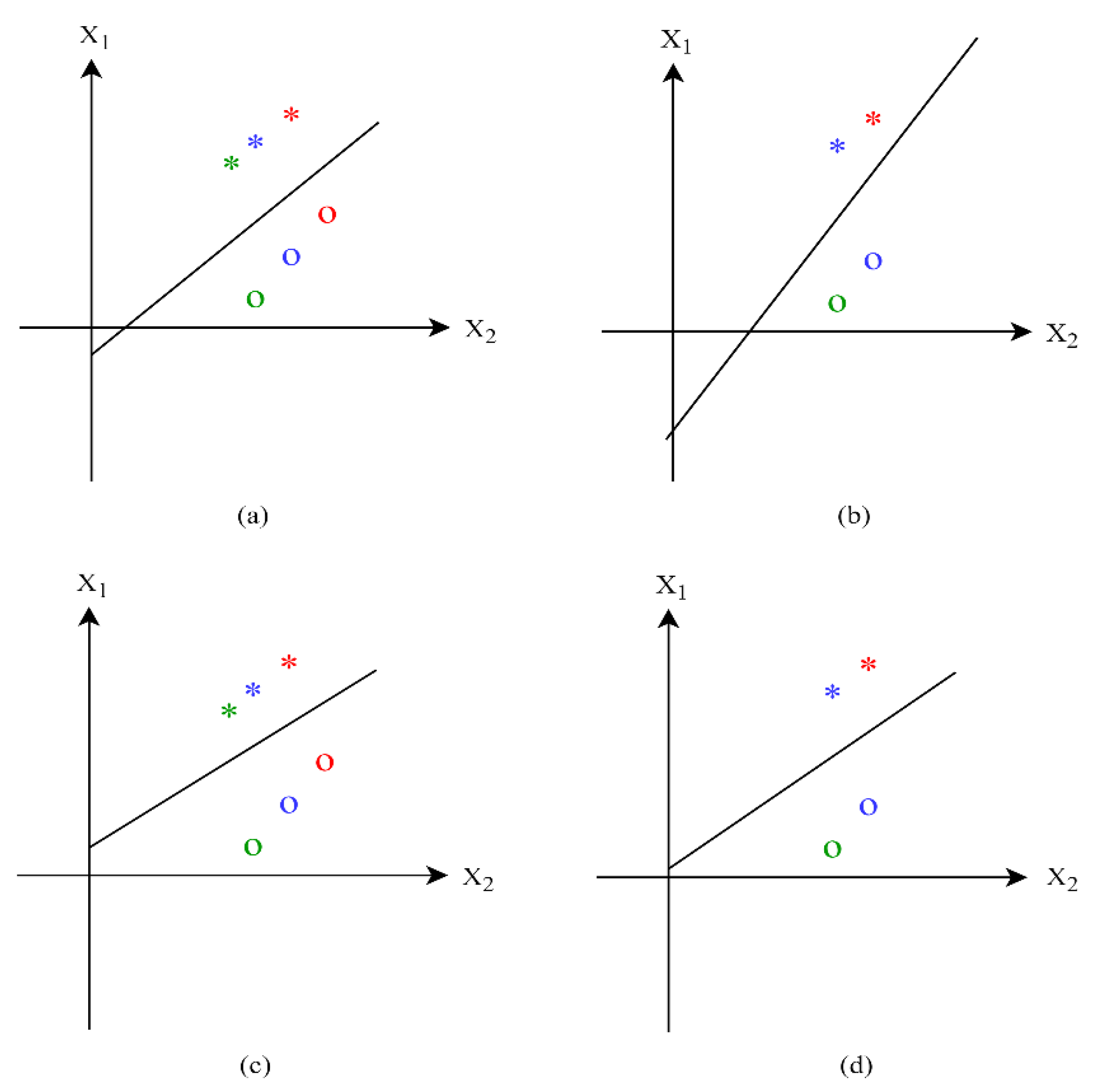
In order to illustrate, a toy example is provided in Figure 5. Consider that we have a dataset with six samples, three of which are in star class and others are in circle class. A logistic regression classifier, as shown in Figure 5a, is trained. If we train the model for a bootstrap dataset in which green star and red circle are omitted, the parameters dramatically change, as shown in Figure 5b. Therefore, it can be concluded that we cannot be certain about the model’s parameters which depend highly on the training set. To make the parameters more stable, the parameters can be regularized. The model will change to Figure 5c. As depicted in Figure 5d, the model would not drastically change after training on the bootstrap set.

4. Logistic Regression

Logistic Regression classification aims to determine the probability that the output variable belongs to a specific class as a function of a linear summation of the features. This function is asserted in (1) and (2) [24]:
Z = ω 0 + ω 1 X 1 + ω 2 X 2 + + ω p X p
P ( G = 1 ) = e Z e Z + 1
In (1) and (2), X1, X2, …, Xp are features. Omegas are coefficients, and P(G = 1) is the probability that output G belongs to class 1. Coefficients should be tuned so that the likelihood that the training samples’ outputs occur is maximized. This can be formulized for a training dataset of R samples such as (3), which can be rewritten as (4):
max ω 0 , ω 1 ,   ω 2 ,   ,   ω p r = 1 R { P ( Z r ) Y r ( 1 P ( Z r ) ) 1 Y r }
min ω 0 , ω 1 ,   ω 2 ,   ,   ω p r = 1 R { Y r . log ( P ( Z r ) ) + ( 1 Y r ) . log ( 1 P ( Z r ) ) }
Several algorithms, such as gradient descent, can be used for optimizing the likelihood [14].

Performance Evaluation

Four performance measures ”Accuracy”, “Precision”, “Recall”, and “F1-Score” are used to evaluate the performance of classifiers. These measures are presented in (5)–(8) [25]:
A c c u r a c y = T P + T N T P + T N + F P + F N
P r e c i s i o n = T P T P + F P
R e c a l l = T P T P + F N
F 1 S c o r e = 2 × P r e c i s i o n × R e c a l l P r e c i s i o n + R e c a l l
In (5)–(7), TP and TN are the number of samples that the classifier truly predicted as positive (class 1) and negative (class 2). FP and FN are the number of samples that the classifier wrongly predicted as positive and negative. For imbalanced datasets, accuracy is not a good evaluation measure. As an illustrative example, consider that there are 10 positive samples and 99,990 negative samples. If a weak classifier labels all samples as negative, the accuracy of the classifier would be 99.99 percent. Therefore, accuracy may overrate the performance of the classifier. The recall measure evaluates what percentage of positive samples are labeled truly. In the example mentioned, this is zero.
On the other hand, the precision measure calculates what percentage of the samples that the algorithm labeled as positive are really positive. Some biased algorithms may have either a large value of recall or a large value of precision. Therefore, the F1-score is calculated in order to represent both recall and precision. If either recall or precision has a small value, F1-Score will also be small.

5. Case Study

The IBM attrition dataset is used as the case study. This dataset consists of 35 columns for each employee. One of these columns, which is “attrition,” is the target output of the classifier. The other 34 columns are features. Two of these features, which are “standard hours” and “employee count,” are constant for all employees. Therefore, they are omitted from the features. Other features are listed as: “age”, “business travel”, “daily rate”, “department”, “distance from home”, “education”, “education field”, “employee number”, “environment satisfaction”, “gender”, “hourly rate”, “job involvement”, “job level”, “job role”, “job satisfaction”, “marital status”, “monthly income”, “monthly rate”, “number companies worked”, “over 18”, “overtime”, “percent salary hike”, “performance rating”, “relationship satisfaction”, “stock option level”, “total working years”, “training times last year”, “work-life balance”, “years at company”, “years in the current role”, “years since last promotion”, and “years with the current manager.”
These features are either categorical or numerical. Since machine learning models cannot deal with categorical features directly, categorical data are converted to binary features using dummy coding [26]. For example, the categorical feature “education field” can be converted into five binary variables, as seen in Table 2.

5.1. Feature Selection

In order to decide which features are the most important, the dataset was initially divided into the training&validation set and the test set. Then, the validation set was separated from the training set. The 1-max-out algorithm was performed in order to determine what features should be omitted. After that, the procedure of randomly separating the validation set and performing 1-max-out repeats itself. After seven iterations, the features that were determined to be omitted more than four times were considered eliminated.
According to results of this procedure, “hourly rate”, “Education Field_HR”, “Monthly income”, “Gender female”, “Department_Research & Development”, “Over18_yes”, “Education”, “Job Level”, “Department_Human Resources”, “Business Travel_Travel_Rarley”, “performance rating”, “Job Role_Manufacturing Director”, “Monthly Rate”, “Education Field_Other”, “Business Travel_Non-Travel”, “Education Field_Marketing”, “Years at Company”, “Department_Sales”, “Over Time_No”, “Education Field_Medical”, “Marital Status_Married” are omitted. These features are not necessarily the least important features for attrition prediction. Some of them are chosen to be deleted because they are absolutely correlated with other features in the dataset. For instance, “Gender female” is one minus “Gender male” feature. For categorical features which are converted to binary features, being eliminated means that being in this category neither increases nor decreases the probability of attrition.

5.2. Final Model

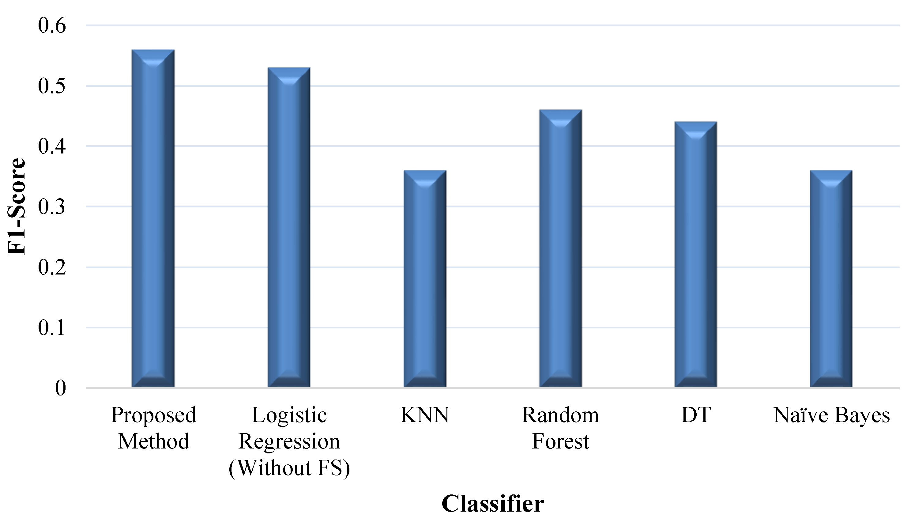
The value of coefficients for each feature is presented in Table 3. According to the coefficients, “years since last promotion”, “overtime”, working as a sales representative, and “number of companies worked” are the most influential factors for an employee to leave the job. With an increase in any of these values, the probability that the employee leaves the job increases. On the other hand, working as a research director, “total working years”, “years with current manager”, and “Job Involvement” are the most influential factors for an employee to stay with the company. The model shows an accuracy of 81% for the test database. The precision, recall, and F1-score are 0.43, 0.82, and 0.56, respectively. If the 1-max-out feature selection were not performed, the accuracy, precision, recall, and F1-score would be 78%, 0.39, 0.82, 0.53, respectively. A comparison of the proposed method’s performance and the classifier used in previous works is displayed in Figure 6. The results show a considerable improvement in F1-score for the proposed method.
It is worth mentioning that these results are valid only for this dataset. These coefficients may vary for other companies in another country with a different culture and economic situation.

5.3. Parameters Confidence Analysis

In order to check the confidence value for each coefficient, the procedure of Section III is performed. Three hundred bootstrap datasets are generated from the original dataset. Then, the model is trained for each dataset. The average, standard deviation, and coefficient of variations (standard deviation to the absolute value of average ratio) of all coefficients are listed in Table 4. The standard deviations show an average level of confidence. We can be more confident for the fields in which the value of the coefficient of variations is small. For instance, we have the most confidence in the coefficient “over time” feature. In contrast, we are not certain about the coefficient associated with the “Job Role_Research Scientist” feature.
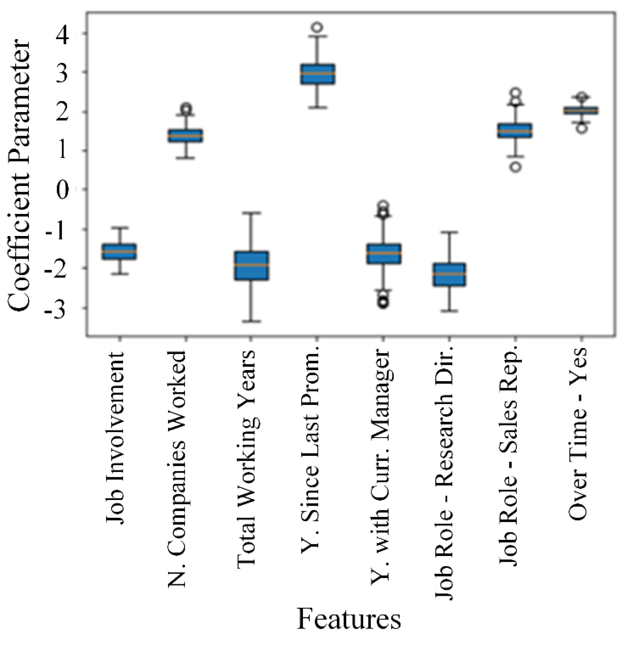
Box plots of the coefficients can also graphically demonstrate the variation of the parameter over all bootstraps. Figure 7 depicts the variation of coefficients associated with the most influential features, which was discussed in the previous subsection. This plot demonstrates that the years since last promotion’s coefficient takes a value between 2 and 4 for all of the bootstrap training datasets. Therefore, we can be confident about its prominent effect on attrition. The coefficient of the “Over Time-Yes” feature barely varies. Therefore, we can be sure about the value of this coefficient. In contrast, the value of the “Years with Current Manager” coefficient varies across a wide interval. Thus, we cannot be certain about this parameter. However, in all of the bootstrap datasets, this parameter is negative. Therefore, it can be inferred that this feature has a good impact on making the employers stay with the company.

6. Conclusions

This paper aimed at presenting a machine learning model for predicting employee attrition. A feature selection method for reducing the dimension of the feature space was first presented. Then, a logistic model was trained for the purpose of prediction. A comparison of the results with the existing methods reveals that the proposed feature selection increases the performance of the predictor. The model demonstrated that “years after the last promotion”, “Over Time—Yes”, “Job Role_Sales Representative”, and “Number Companies Worked” are the prominent reasons for leaving the job. Bigger values for these features lead to a greater attrition probability. Conversely, “total working years”, “years with current manager”, and “job involvement” are the most influential factor for staying with the company. In order to check whether the parameters are valid, 300 hundred bootstrap datasets were produced. For each of these, a model was fitted. Then, a statistical analysis of the coefficient of each feature was performed. Generally, the variation of coefficients was acceptable. In particular, variations in parameters that are associated with the most influential features were insignificant. Therefore, we are sure that the aforementioned features are the prominent features in predicting attrition.
In comparison to previous works, this paper presents a three-stage, pre-processing, processing, and post-processing framework for building a precise employee attrition prediction model and for checking the validity of the model’s parameters. The m-max-out algorithm is introduced for the feature selection at the pre-processing stage. Due to the limits of computation devices that the authors currently face, the 1-max-out (which is a special case in which m is equal to one) is used in this paper. Bigger m could also be used in case of more available computation resources. The validity of the logistic regression model’s parameters for attrition prediction is checked by analyzing the parameters’ variations when they are trained over multiple bootstrap datasets. These preprocessing and post-processing stages can be used to develop accurate and stable models for any kind of general problem. The max-out feature selection method can be used for any set of feature sets, including binary and continuous features. For any kind of Parametric Machine Learning models, statistical analysis of the model’s parameters over numerous bootstraps can infer whether we are confident about the model. For future research on attrition prediction, psychological factors regarding employee attrition are suggested for analysis. In addition, the effect of the number of available vacancies for each employer, considering his specifications and situational factors relating to his/her attrition probability, can also be analyzed in future works.

Author Contributions

Conceptualization, S.N.-Z.; methodology, S.N.-Z.; software, A.A.-N., S.N.-Z.; validation, N.S.-G.; formal analysis, N.S.-G.; investigation, S.N.-Z. and A.A.-N.; resources, N.S.-G.; data curation, N.S.-G., S.H.Z.; writing—original draft preparation, S.N.-Z.; writing—review and editing, A.A.-N., N.S.-G., S.H.Z.; visualization, A.A.-N.; supervision, N.S.-G.; project administration, S.N.-Z.; funding acquisition, N.S.-G., S.H.Z. All authors have read and agreed to the published version of the manuscript.

Funding

This research received no external funding.

Institutional Review Board Statement

The study was conducted according to the guidelines of the Declaration of Helsinki, and approved by the Institutional Review Board (or Ethics Committee) of Amirkabir University of Technology.

Informed Consent Statement

Not Applicable.

Data Availability Statement

Publicly available datasets were analyzed in this study. This data can be found here: https://www.kaggle.com/pavansubhasht/ibm-hr-analytics-attrition-dataset (accessed on 17 April 2021).

Acknowledgments

In this section, you can acknowledge any support given which is not covered by the author contribution or funding sections. This may include administrative and technical support, or donations in kind (e.g., materials used for experiments).

Conflicts of Interest

The authors declare no conflict of interest.

References

  1. Mohri, M.; Rostamizadeh, A.; Talwalkar, A. Foundations of Machine Learning; MIT Press: Cambridge, MA, USA, 2018. [Google Scholar]
  2. Mohbey, K.K. Employee’s Attrition Prediction Using Machine Learning Approaches. In Machine Learning and Deep Learning in Real-Time Applications; IGI Global: Hershey, PA, USA, 2020; pp. 121–128. [Google Scholar]
  3. Ponnuru, S.; Merugumala, G.; Padigala, S.; Vanga, R.; Kantapalli, B. Employee Attrition Prediction using Logistic Regression. Int. J. Res. Appl. Sci. Eng. Technol. 2020, 8, 2871–2875. [Google Scholar] [CrossRef]
  4. Frye, A.; Boomhower, C.; Smith, M.; Vitovsky, L.; Fabricant, S. Employee Attrition: What Makes an Employee Quit? Smu Data Sci. Rev. 2018, 1, 9. [Google Scholar]
  5. Yang, S.; Ravikumar, P.; Shi, T. IBM Employee Attrition Analysis. arXiv 2020, arXiv:2012.01286. [Google Scholar]
  6. Alduayj, S.S.; Rajpoot, K. Predicting employee attrition using machine learning. In Proceedings of the 2018 International Conference on Innovations in Information Technology (IIT), Al Ain, United Arab Emirates, 18–19 November 2018; IEEE: New York, NY, USA, 2018; pp. 93–98. [Google Scholar]
  7. Bhuva, K.; Srivastava, K. Comparative Study of the Machine Learning Techniques for Predicting the Employee Attrition. IJRAR-Int. J. Res. Anal. Rev. 2018, 5, 568–577. IJRAR-Int. J. Res. Anal. Rev. 2018, 5, 568–577. [Google Scholar]
  8. Dutta, S.; Bandyopadhyay, S.K. Employee attrition prediction using neural network cross validation method. Available online: https://www.researchgate.net/profile/Shawni-Dutta/publication/341878934_Employee_attrition_prediction_using_neural_network_cross_validation_method/links/5ed7becf299bf1c67d352327/Employee-attrition-prediction-using-neural-network-cross-validation-method.pdf (accessed on 17 April 2021).
  9. Qutub, A.; Al-Mehmadi, A.; Al-Hssan, M.; Aljohani, R.; Alghamdi, H.S. Prediction of Employee Attrition Using Machine Learning and Ensemble Methods. Int. J. Mach. Learn. Comput. 2021, 11. [Google Scholar] [CrossRef]
  10. Fallucchi, F.; Coladangelo, M.; Giuliano, R.; William De Luca, E. Predicting Employee Attrition Using Machine Learning Techniques. Computers 2020, 9, 86. [Google Scholar] [CrossRef]
  11. Frierson, J.; Si, D. Who’s next: Evaluating attrition with machine learning algorithms and survival analysis. In Proceedings of the International Conference on Big Data, New York, NY, USA, 25–30 December 2018; Springer: Cham, Germany, 2018; pp. 251–259. [Google Scholar]
  12. Pavansubhash. IBM HR Analytics Employee Attrition & Performance, Version 1. 2017. Retrieved on 30 April 2020. Available online: https://www.kaggle.com/pavansubhasht/ibm-hr-analytics-attrition-dataset (accessed on 31 March 2017).
  13. Zebari, R.; Abdulazeez, A.; Zeebaree, D.; Zebari, D.; Saeed, J. A Comprehensive Review of Dimensionality Reduction Techniques for Feature Selection and Feature Extraction. J. Appl. Sci. Technol. Trends 2020, 1, 56–70. [Google Scholar] [CrossRef]
  14. Venkatesh, B.; Anuradha, J. A review of feature selection and its methods. Cybern. Inf. Technol. 2019, 19, 3–26. [Google Scholar] [CrossRef] [Green Version]
  15. Jin, X.; Xu, A.; Bie, R.; Guo, P. Machine Learning Tech-niques and Chi-Square Feature Selec-tion for Cancer Classification Using SAGE Gene Expres-sion Profiles. In Proceedings of the 2006 International Conference on Data Mining for Biomedical Applications, Singapore, 9 April 2006; Springer: Berlin/Heidelberg, Germany, 2006; pp. 106–115. [Google Scholar]
  16. Kwak, N.; Chong-Ho, C. Input Feature Selection by Mutual Information Based on Parzen Window. IEEE Trans. Pattern Anal. Mach. Intell. 2002, 24, 1667–1671. [Google Scholar] [CrossRef] [Green Version]
  17. Moslehi, F.; Haeri, A. A novel feature selection approach based on clustering algorithm. J. Stat. Comput. Simul. 2021, 91, 581–604. [Google Scholar] [CrossRef]
  18. Yan, K.; Zhang, D. Feature selection and analysis on correlated gas sensor data with recursive feature elimination. Sens. Actuators B: Chem. 2015, 212, 353–363. [Google Scholar] [CrossRef]
  19. Demertzis, K.; Tsiknas, K.; Takezis, D.; Skianis, C.; Iliadis, L. Darknet Traffic Big-Data Analysis and Network Management for Real-Time Automating of the Malicious Intent Detection Process by a Weight Agnostic Neural Networks Framework. Electronics 2021, 10, 781. [Google Scholar] [CrossRef]
  20. Duval, B.; Hao, J.K.; Hernandez Hernandez, J.C. A memetic algorithm for gene selection and molecular classification of cancer. In Proceedings of the 11th Annual Conference on Genetic and Evolutionary Computation, New York, NY, USA, 10–14 July 2009; pp. 201–208. [Google Scholar]
  21. Mehrdad, R.; Kamal, B.; Saman, F. A novel community detection based genetic algorithm for feature selection. J. Big Data 2021, 8, 1–27. [Google Scholar]
  22. Kostrzewa, D.; Brzeski, R. 2017, October. The data dimensionality reduction in the classification process through greedy backward feature elimination. In Proceedings of the International Conference on Man–Machine Interactions, Cracow, Poland, 3–6 October 2017; Springer: Cham, Germany, 2017; pp. 397–407. [Google Scholar]
  23. Fish Market. Available online: https://www.kaggle.com/aungpyaeap/fish-market (accessed on 13 June 2019).
  24. Friedman, J.; Hastie, T.; Tibshirani, R. The Elements of Statistical Learning; Series in Statistics; Springer: New York, NY, USA, 2001. [Google Scholar]
  25. Scikit-Learn User Manual. Available online: https://scikit-learn.org/stable/modules/model_evaluation.html#precision-recall-f-measure-metrics (accessed on 12 April 2021).
  26. Daly, A.; Dekker, T.; Hess, S. Dummy coding vs effects coding for categorical variables: Clarifications and extensions. J. Choice Model. 2016, 21, 36–41. [Google Scholar] [CrossRef]
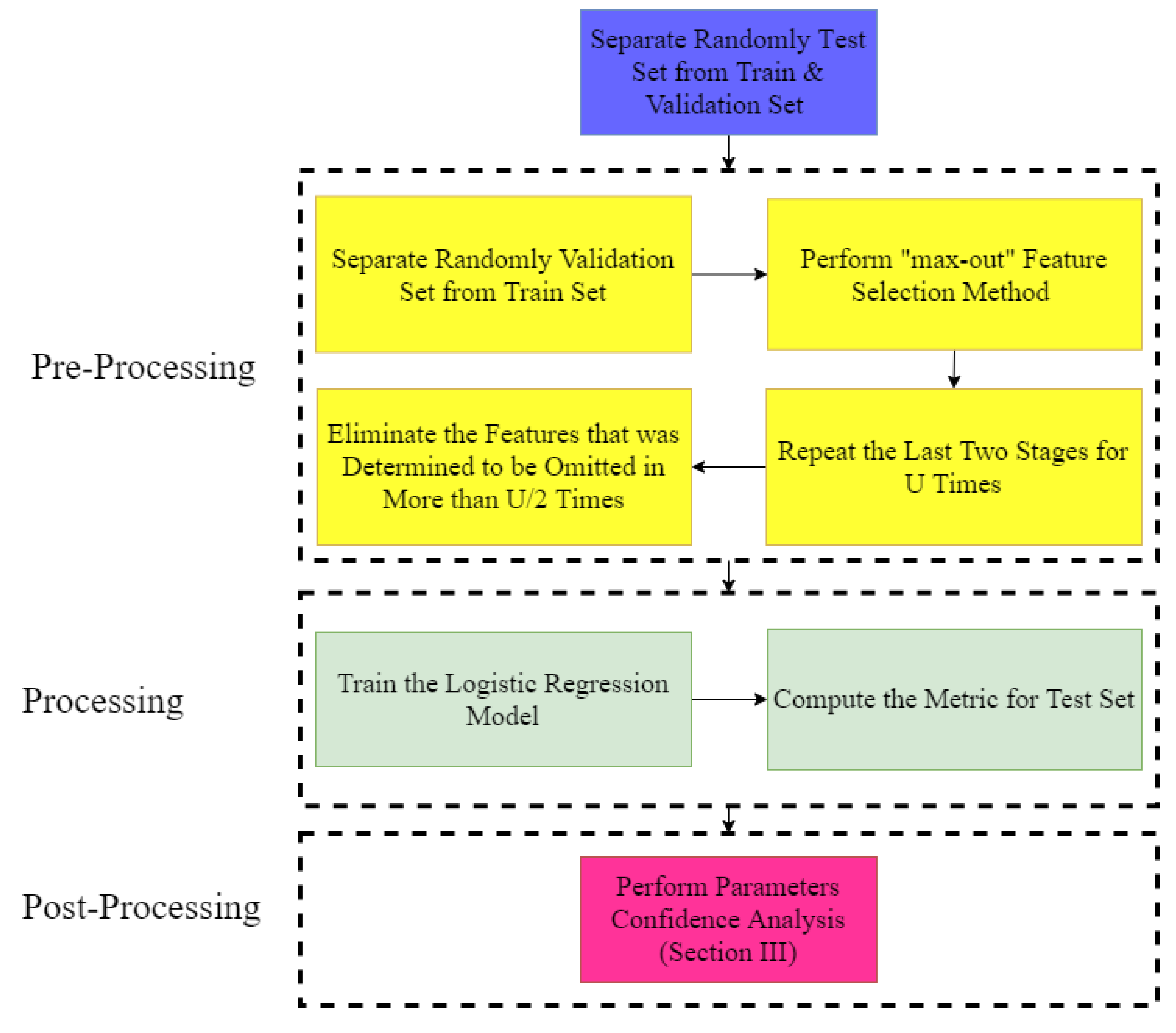
Figure 1. The general structure of the proposed attrition prediction framework.
Mathematics 09 01226 g001
Figure 2. The graphical representation for 1-max-out for an illustrative example.
Mathematics 09 01226 g002
Figure 3. Example of the 1-Max_Out algorithm for the fish market problem.
Mathematics 09 01226 g003
Figure 4. The overall structure of parameter confidence analysis.
Mathematics 09 01226 g004
Figure 5. The overall structure of parameter confidence analysis.
Mathematics 09 01226 g005
Figure 6. Comparison of Different Classifiers’ Performance Measures for the HR Attrition Prediction Task.
Mathematics 09 01226 g006
Figure 7. Confidence level visualization for the most influential coefficients.
Mathematics 09 01226 g007
Table 1. Categories of the feature selection method.
CategoriesExamplesPros.Cons.
Filter[15,16,17]
-
Fast
-
Classifier Independence
-
Less Accurate
Wrapper[18,19]
-
More Accurate
-
Prone to overfitting
Embedded[20]
-
High Accuracy
-
Classifier Specific
Hybrid[21]
-
Higher Accuracy than filters.
-
Less computational Complexity than wrappers
-
Classifier Specific
Table 2. Categorical Feature Education Field Conversion to Binary Features.
Education FieldEF_HREF_LSEF_MaEF_MeEF_Oth
Human Resource10000
Life Science01000
Marketing00100
Medical00010
Other00001
Table 3. Final Model Logistic Regression Coefficients. Green cells are the most important features that contribute to staying with company and red cells are the features that contribute to leave the company the most.
FeatureCoef.FeatureCoef.FeatureCoef.
Age−0.776Environment Satisfaction−1.174Education Field_Life Sciences−0.181
Daily Rate−0.738Business Travel_Travel_Frequently0.810Education Field_Technical Degree0.341
Distance From Home1.004Percent Salary Hike−0.642Training Times Last Year−0.835
Job Involvement−1.536Number Companies Worked1.375Job Role_Laboratory Technician1.009
Relationship Satisfaction−0.701Job Satisfaction−1.116Job Role_Sales Executive0.762
Stock Option Level−0.255Total Working Years−1.887Marital Status_Divorced−0.728
Work Life Balance−0.852Years with Current Manager−1.615Job Role_Manager−0.670
Years in Current Role−1.287Years Since Last Promotion2.925Job Role_Sales Representative1.483
Job Role_Health care Representative−0.333Gender_Male0.606OverTime_Yes1.996
Job Role_Human Resources0.463Job Role_Research Scientist−0.096Job Role_Research Director−2.178
Marital Status_Single0.755Constant2.176
Table 4. Variation of Coefficients Across 300 Bootstrap Datasets. Green cells are the most important features that contribute to staying with the company and red cells are the features that contribute most to leaving the company.
FeatureAve.FeatureAve.FeatureAve.
Std.Std.Std.
CVCVCV
Age−0.786Daily Rate−0.753Distance From Home1.007
0.3200.2210.214
0.4070.2930.212
Environment Satisfaction−1.181Business Travel_Travel_Frequently0.824Job Involvement−1.572
0.1620.1470.235
0.1370.1780.149
Job Satisfaction−1.131Number Companies Worked1.390Percent Salary Hike−0.650
0.1660.2190.228
0.1460.1570.350
Education Field_Life Sciences−0.182Relationship Satisfaction−0.717Stock Option Level−0.262
0.1220.1720.264
0.6700.2391.007
Total Working Years−1.962Training Times Last Year−0.850Education Field_Technical Degree0.358
0.5030.2550.213
0.2560.30.595
Work Life Balance−0.869Years in Current Role−1.308Years Since Last Promotion2.952
0.2200.4030.361
0.2530.3080.122
Years with Current Manager−1.630Gender_Male0.358Job Role_Health care Representative−0.329
0.4090.2130.340
0.2500.5951.03
Job Role_Research Director−2.147Job Role_Human Resources0.450Job Role_Laboratory Technician1.021
0.3710.3510.208
0.1720.780.203
Job Role_Manager−0.622Marital Status_Divorced−0.755Job Role_Research Scientist−0.101
0.2800.1700.192
0.4500.2251.9
Job Role_Sales Executive0.776Job Role_Sales Representative1.500OverTime_Yes2.029
0.2000.2640.124
0.2570.1760.061
Marital Status_Single0.764Constant2.215
0.1700.403
0.2220.182
Publisher’s Note: MDPI stays neutral with regard to jurisdictional claims in published maps and institutional affiliations.