Modeling the Conditional Dependence between Discrete and Continuous Random Variables with Applications in Insurance

Abstract

We jointly model amount of expenditure for outpatient visits and number of outpatient visits by considering both dependence and simultaneity by proposing a bivariate structural model that describes both variables, specified in terms of their conditional distributions. For that reason, we assume that the conditional expectation of expenditure for outpatient visits with respect to the number of outpatient visits and also, the number of outpatient visits expectation with respect to the expenditure for outpatient visits is related by taking a linear relationship for these conditional expectations. Furthermore, one of the conditional distributions obtained in our study is used to derive Bayesian premiums which take into account both the number of claims and the size of the correspondent claims. Our proposal is illustrated with a numerical example based on data of health care use taken from Medical Expenditure Panel Survey (MEPS), conducted by the U.S. Agency of Health Research and Quality.

1. Introduction

The use of bivariate distributions where the marginals are one continuous and the other one discrete are extremely rare in statistics and more specifically in applied statistics. Some examples in which these types of distributions have been previously considered are [1,2,3]. The latter work was applied in tourism settings and the first two papers were applied in actuarial context. Conditional specification structure has also been applied in insurance framework when both marginal distributions are continuous. See [4] for details.

The statistical literature contains numerous methods to obtain bivariate distributions, some of them within the copula framework. These are functions that enable us to separate the marginal distributions from the dependency structure of a given multivariate distribution (see [5,6], among others). Several flexible approaches based on different bivariate copula families such as [7,8,9] have been proposed in the literature, including the Plackett and Frank copulas. The methodology proposed in this work allows us to build a bivariate distribution based on a conditional specification technique (see for instance [10,11]). In general, although the models obtained through this methodology rely on formulations that incorporate many parameters, this requirement can be relaxed, as it will be shown below, to obtain simple and practical expressions. The major advantage of this methodology, as compared to copula approach, is that the latter one incorporates a parameter that controls the correlation which is difficult to estimate, since it is restricted to a range of allowed values.(In practice, this can often be solved by choosing a suitable parametrization (e.g., using the logit or arctan of the correlation as parameter)).

In this work, we jointly model amount of expenditure for outpatient visits and number of outpatient visits by taking into account both dependence and simultaneity. It is noted that both variables are important inputs in the structure of health budgets and in health insurance. More specifically, on the one hand, we model dependence by proposing a bivariate structural model that describes both variables specified in terms of their conditional distributions [10,11]. In fact, the model proposed here is a special case of the one obtained in [3]. On the other hand, simultaneity is implemented into the bivariate distribution, by making two assumptions: $\left(i\right)$ the conditional expectation expenditure for outpatient visits with respect to the number of outpatient visits is linear; and $\left(ii\right)$ the conditional expectation of outpatient visits with respect to the expenditure for outpatient visits is also linear. Thus, we assume that more expenditure implies that the considered health system is capable of handling more visits (note that we are not assuring that more expenditure involves a greater number of visits, which is difficult to sustain in practice); on the other hand, more visits obviously imply more expense.

Furthermore, one of the conditional distributions obtained in our study is used to calculate Bayesian premiums which take into account both the number of claims and the size of the correspondent claim. A credibility expression for the Bayesian premium in which the credibility factor obeys the classical expression provided in [12] is also derived. This type of premiums can be useful in automobile insurance contract to take into consideration both the number of claims and the severity of claim.

The second major contribution of this work is based on the fact that the proposed model enables us to evaluate the effect of covariates on both expenditure and number of visits. Thus, we can distinguish between the effects of these explanatory variables on both responses and, therefore, we can determine which covariates simultaneously affect both expenditure and the number of visits.

The proposed model is empirically evaluated by using data of health care use taken from Medical Expenditure Panel Survey (MEPS), conducted by the U.S. Agency of Health Research and Quality. This set of data can be downloaded from the web page of Professor E. Frees. We jointly model the number of outpatient visits and the amount of expenditure of outpatient visits. Some factors affecting these two random variables will be considered.

The rest of this paper is organized as follows. Section 2 provides the general motivation of this study and the main results. The proposed model for number of visits and expenditure is introduced here. A bivariate model allowing for the implementation of fixed effects is provided in Section 3. Some methods of estimation are shown in Section 4. Next, an empirical analysis of these models is performed in Section 5 and finally Section 6 summarizes the main conclusions drawn from this work.

2. Motivation and Results

In this section, we propose a non-linear bivariate model of amount of expenditure for outpatient visits and number of outpatient visits. The model is a special case of the one provided in [3] which was built by using a characterization via conditional expectations. In this case it was constructed through a class of bivariate distributions such that the conditional distributions belong to a specified exponential family.

As is well known, multivariate distributions can be specified in terms of their conditional distributions rather than directly. In this case, the dependence structure can be modeled using bivariate copulas or other mathematical or statistical methods such as conditional distributions or mixing distributions. By assuming that the conditional distributions belong to certain parametric families of distributions, the joint distribution can be obtained as described in [10] (see also [11] for an introduction to this topic). For  applied works in this setting, see [1,3,13], among others. To obtain the joint distribution, it is first necessary to determine the solution of certain functional equations, which facilitates the derivation of highly flexible multiparametric distributions. As [11] pointed out, when we wish to specify a bivariate distribution it is sometimes convenient to visualize conditional distributions rather than marginal or joint distributions. In this context, it is useful in statistical modeling to have tractable multivariate distributions with given marginals to quantify the dependence effect of the variables in the model.

Accordingly, let us assume that the amount of expenditure for outpatient visits is represented as a random variable X and that the number of outpatients visits to the hospital is also random, and denoted by N. We now wish to obtain the more general bivariate distribution $(X,N)$ whose conditional distributions satisfy the following conditions based on expenditure, conditional on the number of visits and on the number of visits to the hospital conditional to expenditure.

On the one hand, the expenditure for outpatient visits depends on the number of outpatient visits, i.e., if $X|N=n$ is the expenditure conditional to $N=n$ visits is directly proportional to the number of outpatient visits. Hence,

$$\begin{array}{c}\hfill E\left(X\right|N=n)={\alpha }_1+{\alpha }_{2}n,{\alpha }_1>0,{\alpha }_2>0.\end{array}$$

(1)

According to expression (1), assuming that n takes values within the set of integer numbers $\{0,1,\cdots ,n\}$ there is a minimum expense given by ${\alpha }_1$ in the case of no outpatient visits. Then, it seems coherent to assume that the expense increases as the number of visits increases.

On the other hand, it also seems logical to believe that the number of outpatient visits will depend on the expenditure, i.e., the number of outpatient visits that the health care system can assist will depend on its capacity, which in turn is conditioned by the budget (in terms of expenditure) available. Hence,

$$\begin{array}{c}\hfill E\left(N\right|X=x)={\alpha }_{3}x,{\alpha }_3>0.\end{array}$$

(2)

Although Equation (1) includes an intercept since some expenditure would be necessary even for zero visits, pointing out that the health system must be prepared for any future visit, this is not the case of Equation (2). This is mainly due to two reasons: $\left(i\right)$ On the one hand, this modelization facilitates the construction of the mathematical model obtained from Equation (2); and $\left(ii\right)$ it seems obvious that an initial expenditure of near-zero monetary units implies that the health system is unable to absorb patients and, therefore, the mean of visits, and therefore the conditional mean, will be close to zero.

In some circumstances it is certain that this linear dependence relationship is not easily to be assumed. For example, an increase in the number of patient visits to the hospital might be caused by the suffering of more serious diseases that, in turn, incur in more expensive treatments. In this case, it is likely that a non-linear or logarithmic polynomial relationship could be more realistic. Obviously, the modeling in this case would be different from the one considered in this work.

In this work, we propose the use of a bivariate distribution that satisfies the conditions (1) and (2). We will consider the case where one of the conditional random variable is Gamma and the other one Poisson. A discrete random variable is said to follow a Poisson distribution with parameter $\lambda >0$ if its probability mass function (pmf) is given by

$$\begin{array}{c}\hfill f_N\left(n\right)=Pr(N=n)=\frac{{\lambda }^{n}exp(-\lambda )}{n!},n=0,1,2,\cdots \end{array}$$

(3)

In the following, $N\sim \mathcal{P}o\left(\lambda \right)$ will denote a random variable following a Poisson distribution with pmf given by (3). Moreover, a continuous random variable follows a gamma distribution with shape parameter $\alpha >0$ and rate parameter $\beta >0$ if its probability density function (pdf) is expressed as

$$\begin{array}{c}\hfill f_X\left(x\right)=\frac{{\beta }^{\alpha }}{\Gamma \left(\alpha \right)}{x}^{\alpha -1}exp(-\beta x),x>0.\end{array}$$

(4)

We will write in this case, $X\sim \mathcal{G}(\alpha ,\beta )$. By searching for the bivariate conditional distribution, let us now assume that

$$\begin{array}{ccc}\hfill X|N=n& \sim & \mathcal{G}\left(\sigma \right(n),\eta (n\left)\right),\hfill \end{array}$$

(5)

$$\begin{array}{ccc}\hfill N|X=x& \sim & \mathcal{P}o\left(\phi \right(x\left)\right)\hfill \end{array}$$

(6)

for given functions $\phi \left(x\right):\mathbb{N}⟶{\mathbb{R}}^{+}$, $\sigma \left(n\right):{\mathbb{R}}^{+}⟶{\mathbb{R}}^{+}$ and $\eta \left(n\right):{\mathbb{R}}^{+}⟶{\mathbb{R}}^{+}$. Then, the conditional distributions given in (5) and (6) have pdfs given by

$$\begin{array}{ccc}\hfill f_{N|X}\left(N\right|X=x)& =& \frac{1}{n!}exp\left\{-nlog\phi \left(x\right)-\phi \left(x\right)\right\},\hfill \end{array}$$

(7)

$$\begin{array}{ccc}\hfill f_{X|N}\left(X\right|N=n)& =& \frac{\eta {\left(n\right)}^{\sigma \left(n\right)}}{\Gamma \left(\sigma \right(n\left)\right)}exp\left\{-\eta \left(n\right)x+\sigma \left(n\right)logx\right\},\hfill \end{array}$$

(8)

i.e., they are members of the exponential family of distributions. Ref. [3] (see also [10], Chapter 4, p. 98) studied the most general bivariate distribution with conditionals given by (7) and (8) and concluded that this has pdf given by,

$$\begin{array}{c}\hfill f_{X,N}(x,n)=\frac{\kappa {(\beta -\gamma )}^n{x}^{\alpha +\tau n-1}}{n!}exp\left\{-(\beta +\epsilon n)x\right\},\end{array}$$

(9)

with $x>0$, $n=0,1,\cdots ,$ where $\alpha \ge 0$, $\beta >\gamma >0$, $\epsilon \ge 0$ and $\tau \ge 0$. The parameter $\kappa$ is a normalizing constant, a function of the remaining parameters, satisfying

$$\begin{array}{c}\hfill {\kappa }^{-1}={\int }_0^{\infty }\sum _{n=1}^{\infty }\frac{{(\beta -\gamma )}^n{x}^{\alpha +\tau n-1}}{n!}exp\left\{-(\beta +\epsilon n)x\right\}dx,\end{array}$$

which can be obtained from one of the conditional distributions given in (5) and (6), where

$$\begin{array}{ccc}\hfill \sigma \left(n\right)& =& \alpha +\tau n,\hfill \end{array}$$

(10)

$$\begin{array}{ccc}\hfill \eta \left(n\right)& =& \beta +\epsilon n,\hfill \end{array}$$

(11)

$$\begin{array}{ccc}\hfill \phi \left(x\right)& =& (\beta -\gamma )exp\left\{-\epsilon x+\tau logx\right\}.\hfill \end{array}$$

(12)

Certainly, the major limitation of this type of models, built by conditional specification, lies in the difficulty that both the marginal distributions and the joint distribution depend on a normalization constant that in most cases is very difficult or even impossible to calculate in closed form (see for example [14]). Obviously, the difficulty grows when the two variables on which the model depends have different support or it is even more complicated when one variable is discrete and the other one is continuous, as the case considered here. However, from a numerical point of view, this is not an issue of relative importance since there exist integration and summation techniques (more difficult in the latter case) that allow us to compute the constant term. The reader is referred to [15] for more details on how to proceed in these cases.

For practical purposes, an appropriate choice of the parameter could enable us to obtain a closed-form expression for the normalizing constant. For example, the case $\epsilon =\tau =0$ corresponds to that one where N and X are independent and the marginal distributions are Poisson and gamma as in (3) and (4), respectively. The cases $\beta =1+\gamma$, $\epsilon =0$, $\tau =1$ and $\epsilon =0$, $\tau =1$ provide a closed-form model with conditional means of the type of (1) and (2) and thus suitable for our purpose. This latter model that includes an additional parameter as compared to the previous one will be considered here. Then, the bivariate distribution given in (9) can be rewritten as

$$\begin{array}{c}\hfill f_{X,N}(x,n)=\frac{{\left(\gamma x\right)}^{\alpha }{\left[x(\beta -\gamma )\right]}^{n}exp(-\beta x)}{x\Gamma (n+1)\Gamma \left(\alpha \right)},x>0,n=0,1,2,\cdots \end{array}$$

(13)

Please note that the bivariate distribution (13) has a marginal distribution with continuous support and the other one with discrete support. This type of bivariate distribution is uncommon in theoretical and applied statistical literature, allowing us to model phenomena that are not usual in practical situations but sometimes occur, as it is the case described in this paper. See for example [1,16,17].

2.1. Marginal Distributions

The marginal distributions of X and N are given by

$$\begin{array}{ccc}\hfill X& \sim & \mathcal{G}(\alpha ,\gamma ),\alpha >0,\gamma >0,\hfill \\ \hfill N& \sim & \mathcal{NB}\left(\alpha ,p=\frac{\gamma }{\beta }\right),\alpha >0,\beta >\gamma ,\gamma >0,\hfill \end{array}$$

where $\mathcal{NB}$ refers to the negative binomial distribution, i.e.,

$$\begin{array}{ccc}\hfill f_X\left(x\right)& =& \frac{{\gamma }^{\alpha }}{\Gamma \left(\alpha \right)}{x}^{\alpha -1}exp(-\gamma x),x>0,\hfill \\ \hfill f_N\left(n\right)& =& \left(\genfrac{}{}{0pt}{}{\alpha +n-1}{n}\right){\left(\frac{\gamma }{\beta }\right)}^{\alpha }{\left(1-\frac{\gamma }{\beta }\right)}^n,n=0,1,\cdots \hfill \end{array}$$

The marginal distribution of N is obtained by integrating (13) with respect to x over $(0,+\infty )$ and the marginal distribution of X is calculated by summing (13) with respect to n in the support $\{0,1,\cdots \}$.

Furthermore, it is readily apparent that the marginal means and variances are given by

$$\begin{array}{ccc}\hfill E\left(X\right)& =& \frac{\alpha }{\gamma },var\left(X\right)=\frac{\alpha }{{\gamma }^2},\hfill \\ \hfill E\left(N\right)& =& 1+\frac{\alpha }{\gamma }(\beta -\gamma ),var\left(N\right)=\frac{\alpha \beta (\beta -\gamma )}{{\gamma }^2},\hfill \end{array}$$

while the cross moment of X and N is

$$\begin{array}{c}\hfill E\left(XN\right)=\frac{\alpha }{{\gamma }^2}[\beta +\alpha (\beta -\gamma )].\end{array}$$

Simple calculations provide the covariance and the coefficient of correlation. These are given by

$$\begin{array}{ccc}\hfill cov(X,N)& =& \frac{\alpha (\beta -\gamma )}{{\gamma }^2},\hfill \\ \hfill \rho (X,N)& =& \sqrt{1-\frac{\gamma }{\beta }},\hfill \end{array}$$

respectively, which are always positive. The coefficient of correlation is bounded between 0 ($\gamma \approx \beta$) and 1 ($\gamma \approx 0$). Thus, parameter $\gamma$ controls the dependence structure of the model.

If the researcher wanted to work with a model that allows for positive and negative correlations, it would be enough to choose in (9) a less restrictive model.

2.2. Conditional Distributions

The conditional distribution of X given N, shown in (5), is gamma with the parameters given in (10) and (11) and the conditional distribution of N given X, see (6), is Poisson with parameter given in (12). Thus, the conditional distribution of X given $N=n$ is $\mathcal{G}\left(\sigma \right(n),\eta (n\left)\right)$, where

$$\begin{array}{ccc}\hfill \sigma \left(n\right)& =& \alpha +n,\hfill \\ \hfill \eta \left(n\right)& =& \beta \hfill \end{array}$$

and the conditional distribution of N given $X=x$ is $\mathcal{P}o\left(\phi \right(x\left)\right)$, with $\phi \left(x\right)=(\beta -\gamma )x$. Observe that under these conditional distributions, expressions (1) and (2) are guaranteed.

Both the moments and maximum likelihood methods are feasible ways of estimating the vector of parameters $\mathit{\varphi }=(\alpha ,\beta ,\gamma )$ of the distribution through sample observations.

2.3. Hypothesis Testing

By using bivariate data, hypothesis testing can be performed with the parameters $\alpha$, $\beta$ and $\gamma$. We may also be interested in determining, via the likelihood ratio test, when the model might depend only on two parameters, e.g., when $\beta =\gamma +1$. In this case, the vector $\mathit{\varphi }$ can be estimated with the constraint that $\beta =\gamma +1$. If we denote the new vector by ${\mathit{\varphi }}^{\mathbf{\ast }}$, the critical region for the null hypothesis $H_0:\beta =\gamma +1$ is determined from the test statistic

$$\begin{array}{c}\hfill 2\left[\ell (\widehat{\mathit{\varphi }};(\tilde{x},\tilde{n}))-\ell ({\widehat{\mathit{\varphi }}}^{\mathbf{\ast }};(\tilde{x},\tilde{n}))\right],\end{array}$$

which asymptotically has a ${\chi }^2$-squared distribution with one degree of freedom.   

3. Allowing for Covariates

In this section, we introduce a more practical model where covariates may be easily implemented. The bivariate linear regression model, which makes no distributional assumptions, is likely to be unsatisfactory because certain combinations of parameters and regressors could violate the non-negative restriction of the mean of both variables and therefore prediction could give non-realistic values. To avoid this situation, we propose a parametric model based on the distributional assumptions presented in the previous section when the researcher wishes to examine the factors or covariates that can affect simultaneously both means.

For our regression analysis, we reparameterized (13) as a function of its marginal means ${\mu }_1=E\left(X\right)$ and ${\mu }_2=E\left(N\right)$, then $\alpha$ is replaced by $\gamma {\mu }_1$ and $\beta$ is replaced by $\gamma +{\mu }_2/{\mu }_1$, where ${\mu }_1>0$ and ${\mu }_2\ge 1$. Then, the pdf (13) can be rewritten as

$$\begin{array}{c}\hfill f(x,n)=\frac{{\left(x\gamma \right)}^{\gamma {\mu }_1}}{x\Gamma (n+1)\Gamma \left(\gamma {\mu }_1\right)}{\left(\frac{x{\mu }_2}{{\mu }_1}\right)}^{n}exp\left[-\frac{x}{{\mu }_1}({\mu }_2+\gamma {\mu }_1)\right],\end{array}$$

(14)

for $x>0$ and $n=0,1,\cdots$ After this reparameterization we also obtain the cross moment, the covariance and the correlation, which are given by

$$\begin{array}{ccc}\hfill E\left(XN\right)& =& {\mu }_1{\mu }_2+\frac{{\mu }_2}{\gamma },\hfill \\ \hfill cov(X,N)& =& \frac{{\mu }_2}{\gamma },\hfill \\ \hfill \rho (X,N)& =& \sqrt{\frac{{\mu }_2}{\gamma {\mu }_1+{\mu }_2}}.\hfill \end{array}$$

(15)

Thus, parameter $\gamma$ controls the dependence or independence of the model. As $\gamma \to 0$, $\rho (X,N)\to 1$ while $\gamma \to \infty$, $\rho (X,N)\to 0$.

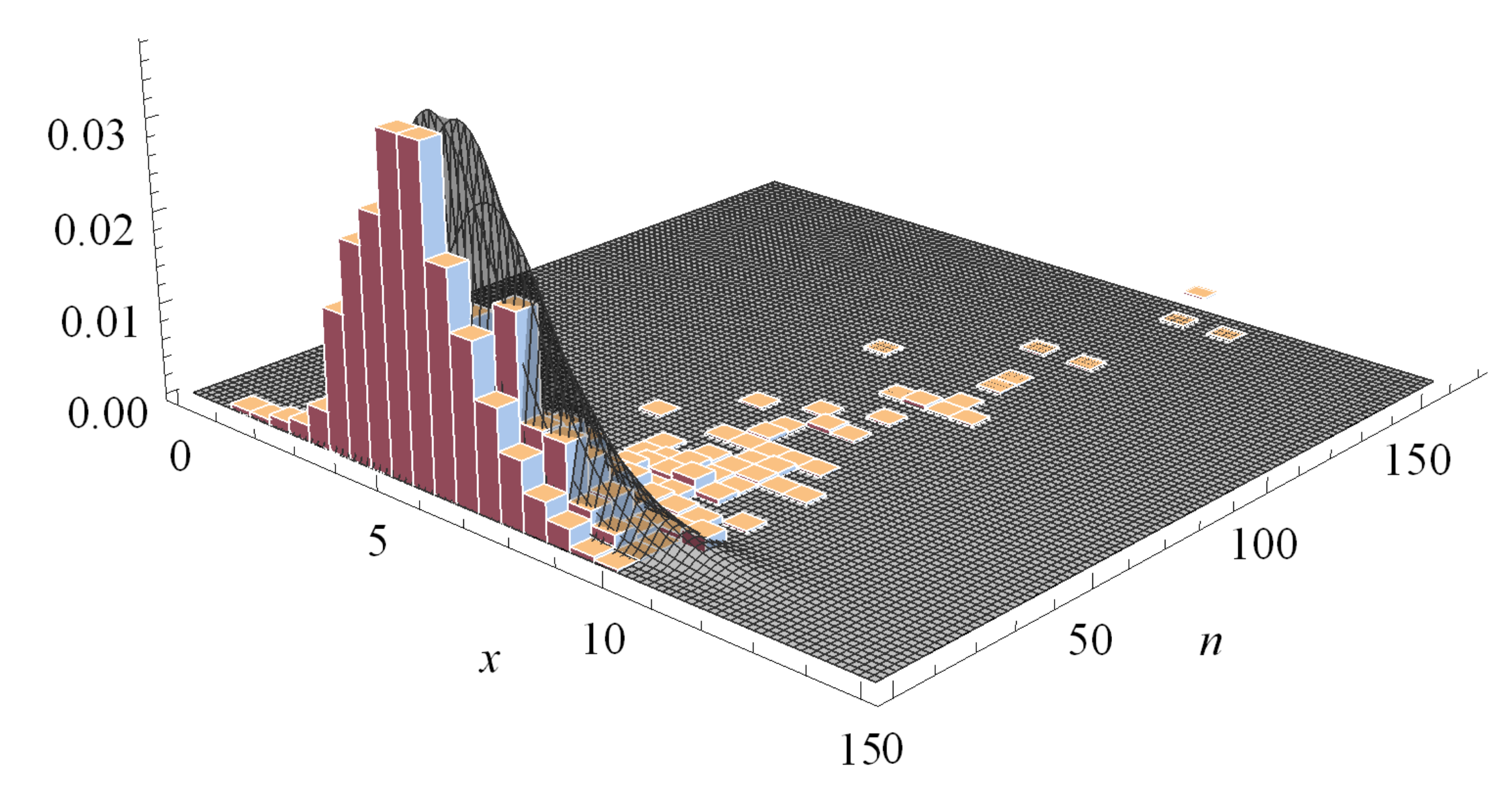
Therefore, the model provided in (14) is suitable for including covariates since the marginal means are given by ${\mu }_1$ and ${\mu }_2$. The expression $(X,N)\sim \mathcal{BGNB}(\gamma ,{\mu }_1,{\mu }_2)$ is used to denote a bivariate random variable $(X,N)$ that follows the distribution given in (14), with marginals gamma and negative binomial. Graphs of the density function for different parameter values and their corresponding contour plots are shown in Figure 1, revealing that the density seems to be unimodal for different values of its parameters.

Figure 1. Graphs of the density for the bivariate distribution $f(x,n)$ in (14) and the corresponding contour plots for different values of the parameters. Left panel $(\gamma ,{\mu }_1,{\mu }_2)=(0.5,25,15)$ and right panel $(\gamma ,{\mu }_1,{\mu }_2)=(0.65,15,25)$.

Now, let ${\mathit{y}}_i={(y_{1i},\cdots ,y_{ki})}^{\prime }$ and ${\mathit{w}}_i={(w_{1i},\cdots ,w_{ki})}^{\prime }$ be two vectors of k covariates associated with the ith observation. They are two vectors of linearly independent regressors that are thought to determine $(x,n)$. For the ith observation, the model takes the form

$$\begin{array}{ccc}\hfill (X_i,N_i)& \sim & \mathcal{BGNB}(\gamma ,{\mu }_{1i},{\mu }_{2i}),\hfill \\ \hfill log\left({\mu }_{1i}\right)& =& {\mathit{y}}_i^{\prime }\mathit{\delta },\hfill \\ \hfill log({\mu }_{2i}-1)& =& {\mathit{w}}_i^{\prime }\mathit{\eta },\hfill \end{array}$$

for $i=1,\cdots ,t$ and where t denotes the number of observations and $\mathit{\delta }={({\delta }_1,\cdots ,{\delta }_k)}^{\prime }$ and $\mathit{\eta }={({\eta }_1,\cdots ,{\eta }_k)}^{\prime }$ the corresponding vectors of regression coefficients.

Moreover, each of the variables, X and N, can be influenced by different factors, hence the explanatory variables that are taken to explain ${\mu }_{\kappa i}$, $\kappa =1,2$, could not be the same. Furthermore, observe that the log link assumed ensures that ${\mu }_{1i}$ falls within the interval $(0,\infty )$ and ${\mu }_{2i}$ within the interval $(1,\infty )$. Furthermore, in practice the model can handle factors that are only related to just one outcome and not to the other one.

In this study, all estimation computations were implemented by using the Wolfram Mathematica (v. 12.0, Wolfram Research Inc., Champaing, IL, USA) and RATS (v. 7.00 Estima, Evanston, IL, USA) software. In the latter case, the approximation given in (16) was used, obtaining the same results as those ones computed with Mathematica. For further information on these software packages, the reader is referred to [18,19].

4. Some Methods of Estimation

In the following, we derive estimators based on the moments and maximum likelihood methods for the model with and without covariates. We also provide closed-form expressions for the Fisher’s information matrix.

4.1. Estimation of the Model without Covariates

The log-likelihood function and the normal equations to provide the corresponding estimates are almost given in closed form. Let us first consider the case of the model without covariates. If 

$$\begin{array}{c}\hfill (\tilde{x},\tilde{n})=\{(x_1,n_1),(x_2,n_2),\cdots ,(x_t,n_t)\}\end{array}$$

is a sample obtained from the distribution with joint density (14) and $\overline{x}=(1/t){\sum }_{i=1}^t{x}_i$, $\overline{n}=(1/t){\sum }_{i=1}^t{n}_i$ and ${\mu }_{12}=(1/t){\sum }_{i=1}^t{x}_i{n}_i$ are the corresponding sample moments, some computations provide the estimators based on these sample moments, which are given by

$$\begin{array}{c}\hfill {\widehat{\mu }}_1=\overline{x},{\widehat{\mu }}_2=\overline{n},\widehat{\gamma }=\frac{{\widehat{\mu }}_2^2}{{\widehat{\mu }}_1({\mu }_{12}-{\widehat{\mu }}_2(1+{\widehat{\mu }}_2))}.\end{array}$$

The Score Vector and Fisher Information Matrix

We now consider the method of maximum likelihood estimation. Let $\Theta =(\gamma ,{\mu }_1,{\mu }_2)$ be the vector of parameters to be estimated. The log-likelihood function is proportional to

$$\begin{array}{ccc}\hfill \ell ((\tilde{x},\tilde{n});\Theta )& \propto & t\left[\gamma {\mu }_1({\overline{x}}^{\ast }+log\gamma )-log\Gamma \left(\gamma {\mu }_1\right)\right]\hfill \\ & & +t\overline{n}\left[log{\mu }_2-log{\mu }_1\right]-\frac{t\overline{x}({\mu }_2+\gamma {\mu }_1)}{{\mu }_1},\hfill \end{array}$$

where ${\overline{x}}^{\ast }=(1/t){\sum }_{i=1}^{t}log{x}_i$.

Thus, the normal equations which provide the estimators of the parameters are given by

$$\begin{array}{ccc}\hfill {\overline{x}}^{\ast }+log\gamma +1-\psi \left(\gamma {\mu }_1\right)-\frac{\overline{x}}{{\mu }_1}& =& 0,\hfill \\ \hfill {\mu }_1^2\gamma \left[{\overline{x}}^{\ast }+log\gamma -\psi \left(\gamma {\mu }_1\right)\right]-{\mu }_1\overline{n}+\overline{x}{\mu }_2& =& 0,\hfill \\ \hfill {\mu }_1\overline{n}-\overline{x}{\mu }_2& =& 0,\hfill \end{array}$$

where $\psi \left(z\right)$ is the digamma function (the logarithmic derivative of the Euler gamma function). After some algebra the maximum likelihood estimators of ${\mu }_1$ and ${\mu }_2$ are obtained, which are given by ${\widehat{\mu }}_1=\overline{x}$ and ${\widehat{\mu }}_2=\overline{n}$. Finally, the estimator of the parameter $\gamma$ is the solution of the equation

$$\begin{array}{c}\hfill log\gamma -\psi \left(\gamma {\widehat{\mu }}_1\right)+{\overline{x}}^{\ast }=0,\end{array}$$

which can be solved numerically.

The second partial derivatives are as follows:

$$\begin{array}{ccc}\hfill \frac{{\partial }^2\ell ((\tilde{x},\tilde{n});\Theta )}{\partial {\gamma }^2}& =& \frac{t{\mu }_1}{\gamma }-t{\mu }_1^2{\psi }_1\left(\gamma {\mu }_1\right),\hfill \\ \hfill \frac{{\partial }^2\ell ((\tilde{x},\tilde{n});\Theta )}{\partial \gamma \partial {\mu }_1}& =& t\left[\overline{1}+x^{\ast }+log\gamma -\psi \left(\gamma {\mu }_1\right)-\gamma {\mu }_1{\psi }_1\left(\gamma {\mu }_1\right)\right],\hfill \\ \hfill \frac{{\partial }^2\ell ((\tilde{x},\tilde{n});\Theta )}{\partial \gamma \partial {\mu }_2}& =& 0,\hfill \\ \hfill \frac{{\partial }^2\ell ((\tilde{x},\tilde{n});\Theta )}{\partial {\mu }_1^2}& =& \frac{t\overline{n}}{{\mu }_1^2}-t{\gamma }^2{\psi }_1\left(\gamma {\mu }_1\right)-\frac{2t\overline{x}}{{\mu }_1^3}{\mu }_2,\hfill \\ \hfill \frac{{\partial }^2\ell ((\tilde{x},\tilde{n});\Theta )}{\partial {\mu }_1\partial {\mu }_2}& =& \frac{t\overline{x}}{{\mu }_1^2},\hfill \\ \hfill \frac{{\partial }^2\ell ((\tilde{x},\tilde{n});\Theta )}{\partial {\mu }_2^2}& =& -\frac{t\overline{n}}{{\mu }_2^2},\hfill \end{array}$$

where ${\psi }_1(·)$ is the first derivative of the digamma function.

The entries of the Fisher’s information matrix, $\mathcal{J}\left(\widehat{\Theta }\right)$, are therefore

$$\begin{array}{ccc}\hfill {\mathcal{J}}_{11}\left(\widehat{\Theta }\right)& =& {\left.E\left(-\frac{{\partial }^2\ell ((\tilde{x},\tilde{n});\Theta )}{\partial {\gamma }^2}\right)\right|}_{\Theta =\widehat{\Theta }}=-\frac{t{\widehat{\mu }}_1}{\widehat{\gamma }}+t{\widehat{\mu }}_1^2{\psi }_1\left(\widehat{\gamma }{\widehat{\mu }}_1\right),\hfill \\ \hfill {\mathcal{J}}_{12}\left(\widehat{\Theta }\right)& =& {\left.E\left(-\frac{{\partial }^2\ell ((\tilde{x},\tilde{n});\Theta )}{\partial \widehat{\gamma }\partial {\widehat{\mu }}_1}\right)\right|}_{\Theta =\widehat{\Theta }}\approx -\sum _{i=1}^{t}log{x}_i-t\left[(1+log\widehat{\gamma }-\psi \left(\widehat{\gamma }{\widehat{\mu }}_1\right)\right.\hfill \\ & & \left.-\widehat{\gamma }{\widehat{\mu }}_1{\psi }_1\left(\widehat{\gamma }{\widehat{\mu }}_1\right)\right],\hfill \\ \hfill {\mathcal{J}}_{13}\left(\widehat{\Theta }\right)& =& {\left.E\left(-\frac{{\partial }^2\ell ((\tilde{x},\tilde{n});\Theta )}{\partial \widehat{\gamma }{\widehat{\mu }}_2}\right)\right|}_{\Theta =\widehat{\Theta }}=0,\hfill \\ \hfill {\mathcal{J}}_{22}\left(\widehat{\Theta }\right)& =& {\left.E\left(-\frac{{\partial }^2\ell ((\tilde{x},\tilde{n});\Theta )}{\partial {\widehat{\mu }}_1^2}\right)\right|}_{\Theta =\widehat{\Theta }}=-\frac{t\left({\widehat{\mu }}_2\right)}{{\widehat{\mu }}_1^2}+t{\widehat{\gamma }}^2{\psi }_1\left(\widehat{\gamma }{\widehat{\mu }}_1\right)\hfill \\ & & +\frac{2t{\widehat{\mu }}_2}{{\widehat{\mu }}_1^2},\hfill \\ \hfill {\mathcal{J}}_{23}\left(\widehat{\Theta }\right)& =& {\left.E\left(-\frac{{\partial }^2\ell ((\tilde{x},\tilde{n});\Theta )}{\partial {\widehat{\mu }}_1{\widehat{\mu }}_2}\right)\right|}_{\Theta =\widehat{\Theta }}=-\frac{t}{{\widehat{\mu }}_1},\hfill \\ \hfill {\mathcal{J}}_{33}\left(\widehat{\Theta }\right)& =& {\left.E\left(-\frac{{\partial }^2\ell ((\tilde{x},\tilde{n});\Theta )}{\partial {\widehat{\mu }}_2^2}\right)\right|}_{\Theta =\widehat{\Theta }}=\frac{t}{{\widehat{\mu }}_2}.\hfill \end{array}$$

Here, $\widehat{\Theta }$ represents the maximum likelihood estimator of $\Theta$. Observe that the analytic expression of $E({\sum }_{i=1}^{t}log{x}_i)$ is not feasible. For computational reasons, for large values of t, this is evaluated by ignoring the expectation operator and replacing it by ${\sum }_{i=1}^{t}log{x}_i$. The asymptotic variance-covariance matrix of $\widehat{\Theta }$ is obtained by inverting the observed information matrix.

The above model has the advantage of its simplicity; however, the normal equations require the use of the digamma function, $\psi \left(z\right)=\frac{d}{dz}log(\Gamma \left(z\right)),z>0$. Although the digamma function is provided in most of the statistical software, in practical situations it is convenient to approximate the digamma function by the following expression,

$$\begin{array}{c}\hfill log\left(\Gamma \left(z\right)\right)\approx \frac{1}{2}log\left(2\pi \right)+\left(z-\frac{1}{2}\right)log\left(z\right)-z+\frac{z}{2}log\left(zsinh\left(\frac{1}{z}\right)\right),\end{array}$$

(16)

which is well known in the statistical literature and it has been proven to perform well in practice.

4.2. Estimation of the Model with Covariates

For the sake of simplicity, we will assume (This assumption is only made to display the normal equations and the Fisher information matrix in a nicer format. In practice, as is well known, the maximum of the likelihood function can be obtained directly by maximizing the logarithm of the likelihood function, and therefore, the covariates used do not have to be the same for the two response variables.) $\mathit{\eta }=\mathit{\delta }$ and write ${\mu }_{1i}={\mu }_{1i}\left(\mathit{\delta }\right)$ and ${\mu }_{2i}={\mu }_{2i}\left(\mathit{\delta }\right)$. Let us also denote $\Theta =(\gamma ,\mathit{\delta })$, thus the log-likelihood function is proportional to

$$\begin{array}{ccc}\hfill \ell ((\tilde{x},\tilde{n});\Theta )& \propto & \gamma \sum _{i=1}^t{\mu }_{1i}log\left(\gamma x_i\right)-\sum _{i=1}^{t}log\Gamma \left(\gamma {\mu }_{1i}\right)\hfill \\ & & +\sum _{i=1}^t{n}_i\left[log{x}_i+log{\mu }_{2i}-log{\mu }_{1i}\right]\hfill \\ & & -\sum _{i=1}^t\frac{x_i}{{\mu }_{1i}}({\mu }_{2i}+\gamma {\mu }_{1i}).\hfill \end{array}$$

Thus, the normal equations, for $i=1,\cdots ,t$, are given by

$$\begin{array}{ccc}\hfill \frac{\partial \ell ((\tilde{x},\tilde{n});\Theta )}{\partial \gamma }& =& \sum _{i=1}^t{\mu }_{1i}\left[1+log\left(\gamma x_i\right)-\psi \left(\gamma {\mu }_{1i}\right)\right]-t\overline{x}=0,\hfill \\ \hfill \frac{\partial \ell ((\tilde{x},\tilde{n});\Theta )}{\partial {\delta }_j}& =& \gamma \sum _{i=1}^t\frac{\partial {\mu }_{1i}}{\partial {\delta }_j}\left[log\left(\gamma x_i\right)-\psi \left(\gamma {\mu }_{1i}\right)\right]\hfill \\ & & +\sum _{i=1}^t{n}_i\left[\frac{1}{{\mu }_{2i}}\frac{\partial {\mu }_{2i}}{\partial {\delta }_j}-\frac{1}{{\mu }_{1i}}\frac{\partial {\mu }_{1i}}{\partial {\delta }_j}\right]\hfill \\ & & -\sum _{i=1}^t\frac{x_i}{{\mu }_{1i}^2}\left[{\mu }_{1i}\frac{\partial {\mu }_{2i}}{\partial {\delta }_j}-{\mu }_{2i}\frac{\partial {\mu }_{1i}}{\partial {\delta }_j}\right]=0,\hfill \end{array}$$

where $j=1,\cdots ,k$, $\frac{\partial {\mu }_{1i}}{\partial {\delta }_j}=y_{ij}{\mu }_{1i}$ and $\frac{\partial {\mu }_{2i}}{\partial {\delta }_j}=w_{ij}{\mu }_{2i}$. Again, the approximation given in (16) can be used instead of the digamma function. Finally, after computing the second partial derivatives we obtain the elements of the Fisher’s information matrix, as follows:

$$\begin{array}{ccc}\hfill {\mathcal{J}}_{11}\left(\widehat{\Theta }\right)& =& {\left.E\left(-\frac{{\partial }^2\ell ((\tilde{x},\tilde{n});\Theta )}{\partial {\gamma }^2}\right)\right|}_{\Theta =\widehat{\Theta }}=-\sum _{i=1}^t{\widehat{\mu }}_{1i}\left[\frac{1}{\widehat{\gamma }}-{\widehat{\mu }}_{1i}{\psi }_1\left(\widehat{\gamma }{\widehat{\mu }}_{1i}\right)\right],\hfill \\ \hfill {\mathcal{J}}_{12}\left(\widehat{\Theta }\right)& =& {\left.E\left(-\frac{{\partial }^2\ell ((\tilde{x},\tilde{n});\Theta )}{\partial \gamma \partial {\delta }_j}\right)\right|}_{\Theta =\widehat{\Theta }}\approx -\sum _{i=1}^t{y}_{ij}{\widehat{\mu }}_{1i}\left[1+log\left(\widehat{\gamma }{x}_i\right)\right.\hfill \\ & & \left.-\psi \left(\widehat{\gamma }{\widehat{\mu }}_{1i}\right)-\widehat{\gamma }{\widehat{\mu }}_{1i}{\psi }_1\left(\widehat{\gamma }{\widehat{\mu }}_{1i}\right)\right],\hfill \\ \hfill {\mathcal{J}}_{22}\left(\widehat{\Theta }\right)& =& {\left.E\left(-\frac{{\partial }^2\ell ((\tilde{x},\tilde{n});\Theta )}{\partial {\delta }_j^2}\right)\right|}_{\Theta =\widehat{\Theta }}\approx -\sum _{i=1}^t\left\{y_{ij}^2{\mu }_{1i}\widehat{\gamma }\left[log\left(\widehat{\gamma }{x}_i\right)-\psi \left(\widehat{\gamma }{\widehat{\mu }}_{1i}\right)\right]\right.\hfill \\ & & \left.-y_{ij}^2{\widehat{\mu }}_{1i}^2{\widehat{\gamma }}^2{\psi }_1\left(\widehat{\gamma }{\widehat{\mu }}_{1i}\right)+x_i\frac{{\mu }_{2i}}{{\mu }_{1i}}{\left(w_{ji}-y_{ji}\right)}^2\right\},\hfill \\ \hfill {\mathcal{J}}_{23}\left(\widehat{\Theta }\right)& =& {\left.E\left(-\frac{{\partial }^2\ell ((\tilde{x},\tilde{n});\Theta )}{\partial {\delta }_j\partial {\delta }_l}\right)\right|}_{\Theta =\widehat{\Theta }}\approx -\sum _{i=1}^t\left\{y_{ij}{y}_{il}\widehat{\gamma }{\widehat{\mu }}_{1i}\left[log\left(\widehat{\gamma }{x}_i\right)-\psi \left(\widehat{\gamma }{\widehat{\mu }}_{1i}\right)\right]\right.\hfill \\ & & \left.-y_{ij}{y}_{il}{\widehat{\mu }}_{1i}^2{\widehat{\gamma }}^2{\psi }_1\left(\widehat{\gamma }{\widehat{\mu }}_{1i}\right)+x_i\frac{{\mu }_{2i}}{{\mu }_{1i}}\left(w_{ij}{w}_{il}-w_{ij}{y}_{il}-y_{ij}{w}_{il}+y_{ij}{y}_{il}\right)\right\},j\ne l.\hfill \end{array}$$

5. Empirical Analysis

To analyze the practical performance of the model proposed, two different examples are provided in this section.

5.1. Example 1

In this first example a set of data that can be downloaded from the web page of Professor E. Frees (https://instruction.bus.wisc.edu/jfrees/jfreesbooks/Regression%20Modeling/BookWebDec2010/data.html) is considered. The dataset contains information about the Medical Expenditure Panel Survey (MEPS), conducted by the U.S. Agency of Health Research and Quality. This survey provides nationally representative estimates of health care use, expenditure, sources of payment, and insurance coverage for the U.S. civilian population. This survey collects detailed information on individuals (Please note that the unit of study is not the individual patient but a health system (public or private) which is the case considered here, although it could also be a hospital unit or similar) of each medical care episode by type of services including physician office visits, hospital emergency room visits, hospital outpatient visits, hospital inpatient stays, all other medical provider visits, and use of prescribed medicines. This detailed information allows the researcher to develop models of health care use to predict future expenditure (see http://www.meps.ahrq.gov/mepsweb/ for more details). We consider MEPS data consisting of 1352 individuals that have positive outpatient expenditure for individuals between ages 18 and 65. In Table 1 the summary of descriptive statistics of these two random variables is displayed. Our dependent variables consist of the logarithm of the amounts of expenditure for outpatient $log\left(EXPENDOP\right)$ visits (i.e., Expenditure) and number of outpatient visits $COUNTOP$, (i.e., Outpatient visits).

Table 1. Summary of descriptive statistics of the two response variables considered.

	Mean	Stand. Dev.	Minimum	Maximum
Expenditure	6.43	1.54	1.09	11.05
Outpatient visits	8.39	14.43	1	167

The degree of association between the two response variables Expenditure and Outpatient visits in the sample for the different levels is summarized in terms of some measures of correlation for bivariate data. In Table 2 Pearson’s, Spearman’s and Kendall’s measures of correlation for these random variables are displayed. It is noticeable that there exists a moderate degree of correlation between these two variables. This is also confirmed by Figure 2 where the scatter plot of these two variables and the theoretical (smoothed) distribution are illustrated. In addition the fitted correlation obtained from (15) by using the maximum likelihood estimates of the parameters provided in Table 3 is 0.592.

Table 2. Pearson’s, Spearman’s and Kendall’s measures of correlation for the two dependent variables considered.

Measure of Correlation	Pearson’s	Spearman’s	Kendall’s
	0.5232	0.7663	0.2856

Figure 2. Empirical (smoothed) distribution (histogram) and theoretical distribution model of the bivariate distribution considered.

Table 3. Parameter estimates, standard errors and negative of the log-likelihood (NLL) for the model without covariates.

Parameter	Estimate	Stand. Error
$\widehat{\gamma }$	2.412	0.094
${\widehat{\mu }}_1$	6.428	0.044
${\widehat{\mu }}_2$	8.394	0.098
NLL	11,014.532
Observations	1352

For the bivariate model without covariates parameters estimates together with their corresponding standard errors are provided in Table 3 by using the parametrization of the bivariate model given in (14). In addition, the minimum value of the negative of the log-likelihood function (NLL) and the total sample size is displayed. Under this parametrization, ${\widehat{\mu }}_1$ and ${\widehat{\mu }}_2$ correspond to the estimates of the marginal means.

Parameter estimates and standard errors for the model with covariates are given below in Table 4 for the continuous random variable, Expenditure, and the discrete one, Outpatient visits. Explanation of the covariates considered can be found at the Data Descriptions file available on the same web page. As it can be seen many explanatory variables are statistically significant at the 5% level. Only the covariates unemploy, i.e., employment status of patients and income, i.e., income compared to poverty line do not have a significant impact simultaneously on the marginal means of the variables Expenditure and Outpatient visits. In addition, the dummy variable high school degree highsch, managedcare, region and marital status, maristat are not significant for the continuous response variable. On the other hand, the explanatory variable race, i.e., race of the patient is not statistically significant at the same level for the Outpatient visits response variable.

Table 4. Parameter estimates, p-values and the log-likelihood (NLL) for the model with covariates.

	Expenditure		Outpatient Visits
Parameter	Estimate	$\mathit{p}$-Value	Estimate	$\mathit{p}$-Value
age	0.119	0.000	0.165	0.000
anylimit	0.075	0.000	0.721	0.000
college	0.014	0.092	0.218	0.000
highsch	−0.002	0.821	0.122	0.000
gender	0.041	0.000	0.253	0.000
mnhpoor	0.047	0.020	0.257	0.000
insure	0.099	0.000	0.105	0.002
usc	0.052	0.001	0.161	0.000
unemploy	−0.000	0.953	0.003	0.885
managedcare	0.008	0.541	−0.127	0.000
famsize	−0.010	0.006	−0.048	0.000
countop	0.070	0.000	0.199	0.000
race	0.017	0.003	0.015	0.148
region	−0.001	0.687	−0.054	0.000
education	0.009	0.033	0.094	0.000
maristat	−0.007	0.219	−0.058	0.000
income	−0.006	0.094	0.002	0.774
physical health	0.028	0.000	0.131	0.000
constant	1.172	0.000	0.594	0.000
$\gamma$	3.052 (0.000)
NLL	9163.372
Observations	1352

5.2. Example 2

By using statistical tools from risk theory, the conditional distribution of N given $X=x$ provided in Section 2 can be used to compute bonus-malus premiums based on both number and size of the claims. The procedure of handling the variables number of claims and their respective claims size in the actuarial literature and, in particular, in automobile insurance, is usually based, given the difficulty involved in their study, on considering both variables separately (see [20,21]). The main advantage provided by the model proposed in this work is that it treats them together by taking into account their positive correlation. Please note that this model differs from the traditional collective risk model where the variable of interest is $S={\sum }_{j=1}^N{X}_i$ and it is assumed that $X_j$ are i.i.d. and independent of the variable N.

Let us now consider that the conditional distribution $N|X=x\sim \mathcal{P}({\mu }_{2}x/{\mu }_1)$ is defined in a way such that ${\mu }_2$ follows a gamma prior distribution with shape parameter $a>0$ and scale parameter $b>0$. Then, it is straightforward that after observing the data $\tilde{n}=(n_1,\cdots ,n_t)$, the posterior distribution of ${\mu }_2$ given the data $\tilde{n}$, is again gamma with updated parameters

$$\begin{array}{ccc}\hfill a^{\ast }& =& a+\sum _{i=1}^t{n}_i,\hfill \end{array}$$

(17)

$$\begin{array}{ccc}\hfill b^{\ast }& =& b+\frac{tx}{{\mu }_1}.\hfill \end{array}$$

(18)

Now, under squared-error loss function the net risk premium is just the mean of the random variable N, depending obviously on x, i.e.,

$$\begin{array}{c}\hfill P(x,{\mu }_1,{\mu }_2)=E\left(N\right|X=x,{\mu }_1,{\mu }_2)=\frac{{\mu }_{2}x}{{\mu }_1}\end{array}$$

and the collective (prior) premium is the mean of the latter one and it results

$$\begin{array}{c}\hfill P=E\left[E\left(N\right|X=x,{\mu }_1,{\mu }_2)\right]=\frac{ax}{b{\mu }_1}.\end{array}$$

(19)

Since the posterior distribution is conjugate with respect to the likelihood, the Bayesian net premium is obtained directly from (19) by using (17) and (18) and results

$$\begin{array}{c}\hfill P^{\ast }=\frac{(a+n^{+})x}{\left(b+\frac{tx}{{\mu }_1}\right){\mu }_1},\end{array}$$

(20)

where $n^{+}={\sum }_{i=1}^t{n}_i$.

In actuarial statistics, the Bayesian premium is a useful premium calculation tool, especially in the automobile insurance sector, since it combines sample information (of an insured) with a priori information (related to the group of insured). This Bayes premium can be easily calculated, i.e., the posterior mean of the parameter ${\mu }_2$, when the prior distribution is conjugated with respect to the likelihood used since it is obtained directly from the collective premium by updating the parameters of this prior obtained from the data.

Observe that expression (20) increases with both the number of claims and the claims size, x. Additionally, this Bayesian premium can be rewritten as

$$\begin{array}{c}\hfill P^{\ast }=Z_t\overline{n}+(1-Z_t)P,\end{array}$$

where $\overline{n}=n^{+}/t$ is the sample mean and

$$\begin{array}{c}\hfill Z_t=\frac{tx}{b{\mu }_1+tx}\end{array}$$

is known in the actuarial literature as the credibility factor. It is straightforward to see that $Z_t\to 0$ as $t\to 0$, $Z_t\to 1$ as $t\to \infty$ and $Z_t=t/(t+K)$ where $K=var\left(E\left(N\right|X=x,{\mu }_1,{\mu }_2)\right)/E\left(var\left(N\right|X=x,{\mu }_1,{\mu }_2)\right)$. Thus, the credibility factor obeys the expression given in [12] (see also [22,23], among others).

A simple application of the methodology used in this paper is provided in the following. We suppose a motor vehicle insurance portfolio with mean value of 1 and 1/2 for the number of claims and the amount of claims, respectively.

Then, the expression (20) has been used to compute the Bayesian premiums of an automobile insurance portfolio for different values of the claim size x, by assuming that the mean of the number of claims is 1 (i.e., $a=b=1$) and that the mean of claims size is ${\mu }_1=0.5$. Then, the Bayesian premiums obtained are shown in Table 5 for different values of the number of claims, $n^{+}={\sum }_{i=1}^t{n}_i$, observed over the time period (usually a year) t.

Table 5. Bayesian premiums for different values of claim size and number of claims.

		${\mathit{n}}^{+}$
$x=0.50$	t	0	1	2	3	4	5
	0	1.00	2.00	3.00	4.00	5.00	6.00
	1	0.50	1.00	1.50	2.00	2.50	3.00
	2	0.33	0.66	1.00	1.33	1.66	2.00
	3	0.25	0.50	0.75	1.00	1.25	1.50
	4	0.20	0.40	0.60	0.80	1.00	1.20
	5	0.16	0.33	0.50	0.66	0.83	1.00
		$n^{+}$
$x=1.00$	t	0	1	2	3	4	5
	0	2.00	4.00	6.00	8.00	10.00	12.00
	1	0.66	1.33	2.00	2.66	3.33	4.00
	2	0.40	0.80	1.20	1.60	2.00	2.40
	3	0.28	0.57	0.85	1.14	1.42	1.71
	4	0.22	0.44	0.66	0.88	1.11	1.33
	5	0.18	0.36	0.54	0.72	0.90	1.09
		$n^{+}$
$x=1.50$	t	0	1	2	3	4	5
	0	3.00	6.00	9.00	12.00	15.00	18.00
	1	0.75	1.50	2.25	3.00	3.75	4.50
	2	0.42	0.85	1.28	1.71	2.14	2.57
	3	0.30	0.60	0.90	1.20	1.50	1.80
	4	0.23	0.46	0.69	0.92	1.15	1.38
	5	0.18	0.37	0.56	0.75	0.93	1.12

It is discernible that for all the values of x, i.e., number of claims, the premium increases with the value of the number of claims, $n^{+}$. In a similar way, the premium decreases with the period of time, t in which the policyholder does not declare a claim. Also, for a fixed value of k and t, the value of the premium increases with claim size x.

6. Final Comments

It is useful in applied statistics to obtain tractable bivariate distributions with given marginals that allow us to quantify the degree of dependence of the variables in the model. Although the most traditionally used methodology has been through copulas, in this article, we have examined this issue by using conditional specification structure. In general, the models derived via this approach, are based on expressions that might incorporate many parameters; however, this requirement may be relaxed to obtain simple and useful expressions. Furthermore, this methodology allows us to derive bivariate distributions with discrete and/or continuous marginals. In addition, one of the conditional distributions obtained in this study is used to calculate Bayesian premiums that take into account both the number of claims and the size of the correspondent claims. Also, a credibility expression for the Bayesian premium was derived. Finally, as a numerical application, an example that jointly explain the amount of expenditure for outpatient visits and number of outpatient visits by taking into account both dependence and simultaneity was considered. The model proposed in this paper enable us to evaluate and distinguish the effect of different explanatory variables on both number of visits and expenditure for outpatient visits.

References

- Gómez-Déniz, E.; Calderín, E. Unconditional distributions obtained from conditional specifications models with applications in risk theory. Scand. Actuar. J. 2014, 7, 602–619. [Google Scholar] [CrossRef]
- Gómez-Déniz, E.; Pérez-Rodríguez, J. Modelling dependence between daily tourist expenditure and length of stay. Tour. Econ. 2020, in press. [Google Scholar]
- Sarabia, J.; Gómez-Déniz, E.; Vázquez-Polo, F. On the use of conditional specification models in claim count distributions: An application to bonus-malus systems. ASTIN Bull. 2004, 34, 85–89. [Google Scholar] [CrossRef][Green Version]
- Sarabia, J.; Castillo, E.; Gómez-Déniz, E.; Vázquez-Polo, F. A class of conjugate priors for log–normal claims based on conditional specification. J. Risk Insur. 2005, 72, 479–495. [Google Scholar] [CrossRef]
- Sklar, A. Fonctions de répartition á n dimensions et leurs marges. Publ. Inst. Stat. Univ. Paris 1959, 8, 229–231. [Google Scholar]
- Sklar, A. Random variables, joint distributions, and copulas. Kybernetika 1973, 9, 449–460. [Google Scholar]
- Farlie, D. The performance of some correlation coeficients for a general bivariate distribution. Biometrika 1960, 47, 307–323. [Google Scholar] [CrossRef]
- Gumbel, E. Bivariate exponential distributions. J. Am. Stat. Assoc. 1960, 55, 698–707. [Google Scholar] [CrossRef]
- Morgenstern, D. Einfache beispiele zweidimensionaler verteilungen. Mitt. Math. Stat. 1956, 8, 234–235. [Google Scholar]
- Arnold, B.; Castillo, E.; Sarabia, J. Conditional Specification of Statistical Models; Springer: New York, NY, USA, 1999. [Google Scholar]
- Arnold, B.; Strauss, D. Bivariate distributions with conditionals in prescribed exponential families. J. R. Stat. Soc. 1991, 53, 365–375. [Google Scholar] [CrossRef]
- Bühlmann, H. Experience rating and credibility. ASTIN Bull. 1967, 4, 199–207. [Google Scholar] [CrossRef]
- Sarabia, J.; Castillo, E. Bivariate distributions based on the generalized three-parameter Beta distribution. In Advances on Distribution Theory, Order Statistics and Inference; Balakrishnan, N., Castillo, E., Sarabia, J., Eds.; Birkhäuser: Boston, MA, USA, 2006; Chapter 2; pp. 85–110. [Google Scholar]
- Moschopoulos, P.; Staniswalis, J.G. Estimation given conditionals from an exponential family. Am. Stat. 1994, 48, 271–275. [Google Scholar]
- Davis, P.; Rabinowitz, P. Methods of Numerical Integration; Academic Press: San Diego, CA, USA, 1984. [Google Scholar]
- Kotz, S.; Balakrishnan, N.; Johnson, N. Continuous Multivariate distributions. In Models and Applications; John Wiley and Sons: New York, NY, USA, 2000; Volume 1. [Google Scholar]
- Spanos, A. Probability Theory and Statistical Inference; Cambridge University Press: Cambridge, UK, 1999. [Google Scholar]
- Brooks, C. RATS Handbook to Accompany Introductory Econometrics for Finance; Cambridge University Press: Cambridge, UK, 2009. [Google Scholar]
- Ruskeepaa, H. Mathematica Navigator. Mathematics, Statistics, and Graphics, 4th ed.; Academic Press: Cambridge, MA, USA, 2009. [Google Scholar]
- Frangos, N.; Vrontos, S. Design of optimal Bonus-Malus systems with a frequency and a severity component on an individual basis in automobile insurance. ASTIN Bull. 2001, 31, 1–22. [Google Scholar] [CrossRef]
- Mert, M.; Saykan, Y. On a bonus malus system where the claim frequency distribution is geometric and the claim severity distribution is Pareto. Hacet. J. Math. Stat. 2005, 34, 75–81. [Google Scholar]
- Bühlmann, H.; Gisler, A. A Course in Credibility Theory and its Applications. Springer: Berlin/Heidelberg, Germany, 2005. [Google Scholar]
- Gómez-Déniz, E. A generalization of the credibility theory obtained by using the weighted balanced loss function. Insur. Math. Econ. 2008, 42, 850–854. [Google Scholar] [CrossRef]
Publisher’s Note: MDPI stays neutral with regard to jurisdictional claims in published maps and institutional affiliations. |
© 2020 by the authors. Licensee MDPI, Basel, Switzerland. This article is an open access article distributed under the terms and conditions of the Creative Commons Attribution (CC BY) license (http://creativecommons.org/licenses/by/4.0/).