Dispersion Trading Based on the Explanatory Power of S&P 500 Stock Returns

Abstract

This paper develops a dispersion trading strategy based on a statistical index subsetting procedure and applies it to the S&P 500 constituents from January 2000 to December 2017. In particular, our selection process determines appropriate subset weights by exploiting a principal component analysis to specify the individual index explanatory power of each stock. In the following out-of-sample trading period, we trade the most suitable stocks using a hedged and unhedged approach. Within the large-scale back-testing study, the trading frameworks achieve statistically and economically significant returns of 14.52 and 26.51 percent p.a. after transaction costs, as well as a Sharpe ratio of 0.40 and 0.34, respectively. Furthermore, the trading performance is robust across varying market conditions. By benchmarking our strategies against a naive subsetting scheme and a buy-and-hold approach, we find that our statistical trading systems possess superior risk-return characteristics. Finally, a deep dive analysis shows synchronous developments between the chosen number of principal components and the S&P 500 index.

1. Introduction

Relative value trading strategies, often referred to as statistical arbitrage, were developed by Morgan Stanley’s quantitative group in the mid-1980s and describe a market neutral trading approach [1]. Those strategies attempt to generate profits from the mean reversion of two closely related securities that diverge temporarily. Pairs trading, which in its plain form tries to exploit mispricing between two co-moving assets, is probably the most popular delta-one trading approach amongst relative value strategies. Several studies show that those procedures generate significant and robust returns (see [2,3,4,5,6]).

In the non-linear space, relative value strategies are also prominent. Dispersion approaches are one of the most common trading algorithms and attempt to profit from implied volatility spreads of related assets and changes in correlations. Since index options usually incorporate higher implied volatility and correlation than an index replicating basket of single stock options, returns are generated by selling index options and buying the basket. Ultimately, the trader goes long volatility and short correlation [7]. As shown by [8,9], volatility based strategies generate meaningful and reliable returns. Dispersion trades are normally conducted by sophisticated investors such as hedge funds [10]. In 2011, the Financial Times speculated that Och-Ziff Capital Management (renamed to Sculptor Capital Management, Inc. New York, NY, USA in 2019 with headquarter in New York City, United States), an alternative asset manager with $$34.5$bn total assets under management [11], set up a dispersion trade worth around $$8.8$bn on the S&P 100 index [12]. In academia, References [13,14,15] examined the profitability of dispersion trades and delivered evidence of substantial returns across markets. However, Reference [16] reported that returns declined after the year 2000 due to structural changes in options markets. References [14,15,16] enhanced their returns by trading dispersion based on an index subset. All of those studies try to replicate the index with as few securities as possible, but neglect the individual explanatory power of stocks in their weighting schemes. This provides a clear opportunity for further improvements of the subsetting procedure.

This manuscript contributes to the existing literature in several aspects. First, we introduce a novel statistical approach to select an appropriate index subset by determining weights based on the individual index explanatory power of each stock. Second, we provide a large-scale empirical study on a highly liquid market that covers the period from January 2000 to December 2017 and therefore includes major financial events such as 9/11 and the global financial crisis. Third, we benchmark our statistical trading approaches against baseline dispersion trading algorithms and a buy-and-hold strategy. Fourth, we conduct a deep dive analysis, including robustness, risk factor, and sub-period analysis, that reports economically and statistically significant annual returns of 14.51 percent after transaction costs. Our robustness analysis suggests that our approach produces reliable results independent of transaction costs, reinvestment rate, and portfolio size. Fifth, we evaluate in depth our innovative selection process and report the number of required principal components and selected sector exposures over the study period. We find a synchronous relationship between the number of principal components that are necessary to describe 90 percent of the stock variance and the S&P 500 index performance, i.e., if the market performs well, more components are required. Finally, we formulate policy recommendations for regulators and investors that could utilize our approach for risk management purposes and cost-efficient dispersion trade executions.

The remainder of this paper is structured as follows. Section 2 provides the underlying theoretical framework. In Section 3, we describe the empirical back-testing framework followed by a comprehensive result analysis in Section 4. Finally, Section 5 concludes our work, provides practical policy recommendations, and gives an outlook of future research areas.

2. Theoretical Framework

This section provides an overview of the theoretical framework of our trading strategy. Section 2.1 describes the underlying methodology and the drivers of dispersion trades. Different dispersion trading structures and enhancement methods are elaborated in Section 2.2.

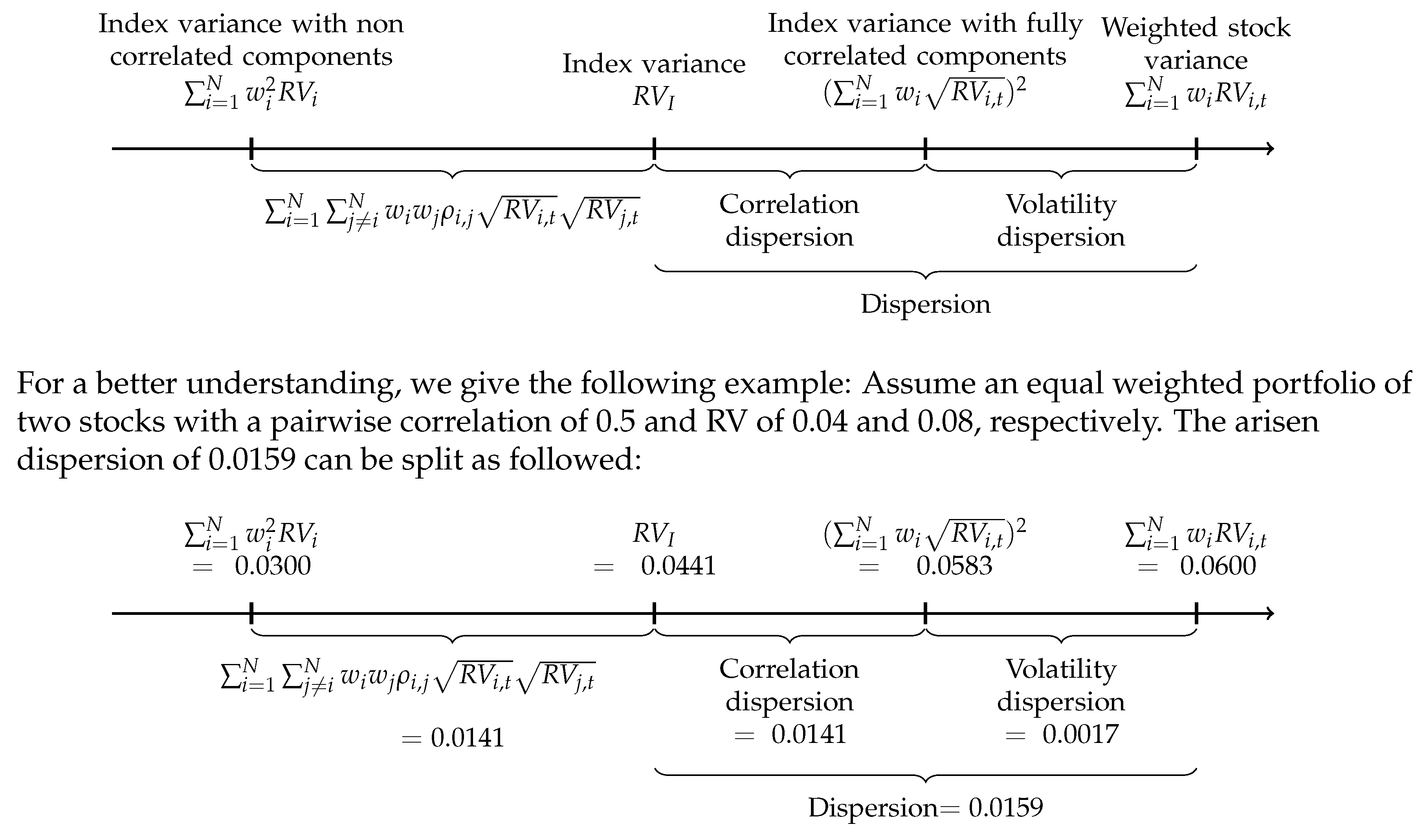
2.1. Dispersion Foundation and Trading Rational

The continuous process of stock price S is defined as [17]:

$$\begin{array}{c}\hfill {\displaystyle \frac{d{S}_t}{S_t}}=\mu \left(t\right)dt+\sigma \left(t\right)d{Z}_t,\end{array}$$

(1)

where the $dt$ term represents the drift and the second term denotes the diffusion component. In one of its simplest forms, continuous processes follow a constant drift $\mu$ and incorporate a constant volatility $\sigma$. In various financial models, for example in the well-known Black–Scholes model (see [18]), it is assumed that the underlying asset follows a geometric Brownian motion (GBM):

$$\begin{array}{c}\hfill d{S}_t=\mu S_{t}dt+\sigma S_{t}d{W}_t.\end{array}$$

(2)

Following [19,20], we define return dispersion for an equity index at time t as:

$$R{D}_t=\sqrt{\sum _{i=1}^N{w}_i{\left(R_{i,t}-R_{I,t}\right)}^2}=\sqrt{\sum _{i=1}^N{w}_i{R}_{i,t}^2-R_{I,t}^2},$$

(3)

where N represents the number of index members, $w_i$ the index weight, and $R_{i,t}$ the return of stock i at time t. Moreover, $R_{I,t}$ denotes the index return with $R_{I,t}={\sum }_{i=1}^N{w}_i{R}_{i,t}$. Return dispersion statistically describes the spread of returns in an index. References [21,22,23] showed in their seminal works that the realized variance (RV) is an accurate estimator of the actual variance (${\sigma }^2$) as RV converges against the quadratic variation. Therefore, RV and ${\sigma }^2$ are used interchangeably in the following. Applying the definition of realized variance of the last J returns $R{V}_{i,t}={\sum }_{k=1}^J{R}_{i,t-k}^2$, Equation (3) can be rewritten as:

$$R{D}_t^2=\sum _{i=1}^N{w}_{i}R{V}_{i,t}-R{V}_{I,t}.$$

(4)

Expanding Equation (4) by the index variance of perfectly correlated index constituents yields:

$$\begin{array}{cc}\hfill R{D}_t^2& =\left(\sum _{i=1}^N{w}_{i}R{V}_{i,t}-{\left(\sum _{i=1}^N{w}_i\sqrt{R{V}_{i,t}}\right)}^2\right)+\left({\left(\sum _{i=1}^N{w}_i\sqrt{R{V}_{i,t}}\right)}^2-R{V}_{I,t}\right).\hfill \end{array}$$

(5)

The first term represents the variance dispersion of the single index constituents. This component is independent of the individual correlations. However, the second expression depends on realized correlations and describes the spread between the index variance under perfectly positively correlated index members and the realized correlations. Therefore, dispersion trades are exposed to volatility and correlation. This is reasonable as the variance of the index is eventually a function of the realized correlations between index members and their variances. Reference [24] already quantified this relationship in 1952:

$$\begin{array}{c}\hfill {\sigma }_I^2=\sum _{i=1}^N{w}_i^2{\sigma }_i^2+\sum _{i=1}^N\sum _{j\ne i}^N{w}_i{w}_j{\sigma }_i{\sigma }_j{\rho }_{i,j},\end{array}$$

(6)

where ${\sigma }_i$ (${\sigma }_j$) represents the volatility of stock i (j) and ${\rho }_{i,j}$ denotes the correlation coefficient between shares i and j.

Figure 1 illustrates the dispersion drivers graphically. Dispersion consists of volatility and correlation dispersion, i.e., the deviation of the realized correlation from perfectly positively correlated index members. The missing diversification benefits of the index compared to uncorrelated constituents decrease the profit of a dispersion trade, highlighting the short correlation characteristic of a long dispersion trade. Hence, a long dispersion trade profits from an increase in individual stock volatility and a decrease in index volatility, which itself implies a decline in correlation. Shorting dispersion leads to a gain when index volatility rises while the constituent’s volatility remains unchanged or falls. In practice, multiple ways exist to structure dispersion trades that possess distinct merits. In our empirical study in Section 3, we develop a cost-efficient way to trade dispersion. Within the scope of this work, we focus on two trading approaches, namely at-the-money (ATM) straddles with and without delta hedging. Both strategies rely on options to trade volatility. When expressing a view on dispersion using non-linear products, one has to consider the implied volatility (IV), which essentially reflects the costs of an option. Profits from owning plain vanilla options are generally achieved when the realized volatility exceeds the implied one due to the payoff convexity. The contrary applies to short positions since these exhibit a concave payoff structure. Thus, a long dispersion trade would only be established if the expected realized volatility exceeds the implied one.

Two essential metrics exist for measuring the implied costs of dispersion trades. First, the costs can be expressed as implied volatility. To assess the attractiveness of a trade, the IV of the index has to be compared with that of the index replicating basket. This method has to assume an average correlation coefficient in order to calculate the IV of the basket. To estimate the average correlation, historical realizations are often used. Second, implied costs can also be directly expressed as average implied correlation, which is computed based on the IVs of the index and its constituents. This measurement simply backs out the average implied correlation so that the IV of the basket equals the index IV. Through modification of the Markowitz portfolio variance equation (see Equation (6)) and assuming $\rho ={\rho }_{i,j}$ for $i\ne j$ and $i,j=1,...,N$, the implied volatility can be expressed as average implied correlation (see [16]):

$$\begin{array}{c}\hfill \overline{\rho }={\displaystyle \frac{{\sigma }_I^2-{\sum }_{i=1}^N{w}_i^2{\sigma }_i^2}{{\sum }_{i=1}^N{\sum }_{j\ne i}^N{w}_i{w}_j{\sigma }_i{\sigma }_j}}.\end{array}$$

(7)

Figure 2 reports the effect of correlation on index volatility in a simple two stock portfolio case. It is easily perceivable that the index variance decreases with a lower correlation of the two stocks. If the two assets are perfectly negatively correlated, the index variance is virtually zero. This represents the best case for a long dispersion trade as the single index constituents variance is unaffected at $0.0064\%$, while the index is exposed to $0\%$ variance. This state generates in the simulation a return dispersion of $0.0800\%$. Nevertheless, this extreme case is not realistic as indices normally incorporate more than two securities. Adding an additional stock leads inevitably to a positive linear relationship with one or the other constituent. Moreover, stocks are typically positively correlated as they exhibit similar risk factors.

The representation of implied costs as average implied correlation is a useful concept as it enables us to assess deviations of index and basket IV by solely computing one figure that is independent of the index size. Hence, this metric is always one-dimensional. Typically, the implied average correlation is compared with historical or forecasted correlations to identify profitable trading opportunities [13,16]. We included this trading filter in our robustness check in Section 4.4 to examine if it is economically beneficial to trade conditional on correlation. Overall, investors would rather sell dispersion in an environment of exceptionally low implied correlation than to build a long position since correlation is expected to normalize in the long run.

However, most of the time investors engage in long dispersion trades. This has mainly two reasons. First, a historical overpricing of implied volatility of index options compared to that of its constituents is persisting. Thus, selling index options is more attractive than buying them. Second, index option sellers can generate profits from the embedded correlation risk premium. Buying index options is ultimately an insurance against decreasing diversification as correlations tend to rise in market downturns. An increase in correlation negatively affects any portfolio diversification. Therefore, many investors are willing to pay a premium to hedge against rising correlations, making long dispersion trades more attractive [25,26]. Nonetheless, Reference [16] showed that the correlation risk premium seems to play only a minor role in explaining the performance of dispersion trades and concluded that returns depend mainly on mispricing and market inefficiency.

Over the years, several explanations for the overpricing of index options have emerged. The most prominent argument is related to the supply and demand of index and stock options. Changes in implied volatility are rooted in net buying and selling pressure. Amongst institutional investors, there is usually high demand for index options, especially puts, to hedge their portfolios. This creates net buying pressure, resulting in a higher implied volatility for index options [27,28,29]. Hedge funds and other sophisticated investors engage in call and put underwriting on single stock options to earn the negatively embedded volatility premium [30]. Due to consistent overpricing, selling both insurance (puts) and lottery tickets (calls) generates positive net returns in the long run, despite a substantial crash risk [31]. Hence, sophisticated market participants would sell volatility especially when the implied volatility is high. This was for example the case after the bankruptcy of Long-Term Capital Management in 1998 when several investors sold the high implied volatility [32]. The net buying pressure for index options and net selling pressure for stock options create the typical mispricing between index IV and the IV of a replicating portfolio. Dispersion trades therefore help balance the supply and demand of index and single name options as the strategy involves buying the oversupplied single stock options and selling the strongly demanded index options. In a long dispersion trade, investors ultimately act as the liquidity provider to balance single stock and index volatility.

2.2. Dispersion Trading Strategies

In the market, a variety of structures to capture dispersion are well established. In this subsection, we give an overview of the two most common variations, namely at-the-money straddles (Section 2.2.1) and at-the-money straddles with delta hedging (Section 2.2.2).

2.2.1. At-The-Money Straddle

One of the traditional and most transparent, as well as liquid ways to trade volatility is by buying and selling ATM straddles. A long straddle involves a long position in a call and put with the same strike price (K) and maturity (T). Selling both options results in a short straddle. The payoff of a long straddle position at T with respect to the share price ($S_T$) is given by:

$$\begin{array}{c}\hfill P_T=\underset{\mathrm{Call}}{\underbrace{{[S_T-K]}^{+}}}+\underset{\mathrm{Put}}{\underbrace{{[K-S_T]}^{+}}},\end{array}$$

(8)

where ${\left[x\right]}^{+}$ represents $max(x,0)$. Translating an ATM straddle into the context of a long dispersion trade, the payoff equals:

$$\begin{array}{c}\hfill P_{T,Dispersion}=\sum _i^N{w}_i\left({[S_{i,T}-K_i]}^{+}+{[K_i-S_{i,T}]}^{+}\right)-\left({[S_{I,T}-K_I]}^{+}+{[K_I-S_{I,T}]}^{+}\right).\end{array}$$

(9)

The first part denotes the single stock option portfolio while the second term corresponds to the index leg. When setting up an at-the-money straddle, the initial delta of the position is approximately zero as the put and call delta offset each other [7]. Despite the low delta at inception, this structure is exposed to directional movements and is therefore not a pure volatility play. This is rooted in changes of the position’s overall delta as the underlying moves or the time to maturity decreases.

2.2.2. At-the-Money Straddle with Delta Hedging

Delta hedging eliminates the directional exposure of ATM straddles. Through directional hedging, profits from an increase in volatility are locked in. Therefore, this structure generates income even in the case that the underlying ends up at expiry exactly at-the-money. The volatility profits are generated through gamma scalping. A long gamma position implies buying shares of the asset on the way down and selling them on the way up [7]. This represents every long investor’s goal: buying low and selling high. A net profit is generated when the realized volatility is higher than the implied volatility at inception as more gamma gains are earned as from the market priced in. Hence, ATM straddles with frequent delta hedging are better suited to trade volatility than a plain option.

Assuming the underlying time series follows a GBM (Equation (2)) and the Black–Scholes assumptions hold, it can be shown that the gamma scalping gains are exactly offset by the theta bleeding when the risk-free rate equals zero [18,33]. Taking the Black–Scholes PDE:

$$\begin{array}{c}\hfill {\displaystyle \frac{\partial \Pi }{\partial t}}+rS{\displaystyle \frac{\partial \Pi }{\partial S}}+{\displaystyle \frac{1}{2}}{\sigma }^2{S}^2{\displaystyle \frac{{\partial }^2\Pi }{\partial S^2}}=r\Pi \end{array}$$

(10)

and substituting the partial derivatives with the Greeks yields:

$$\begin{array}{c}\hfill \Theta +rS\Delta +{\displaystyle \frac{1}{2}}{\sigma }^2{S}^2\Gamma =r\Pi .\end{array}$$

(11)

Invoking Itô’s lemma, this can be expressed for an infinitesimal small time change $dt$ as:

$$\begin{array}{c}\hfill \Theta dt=-{\displaystyle \frac{1}{2}}{\sigma }^2{S}^2\Gamma dt.\end{array}$$

(12)

In the above-mentioned equations, $\Pi$ describes the delta neutral portfolio, S represents the asset price, r illustrates the risk-free interest rate, and $\Theta$ and $\Gamma$ denote the option’s price sensitivities with respect to the passage of time and delta.

In the real world when using a discrete delta hedging method, theta and gamma do not necessarily offset each other. This results partially from the risk and randomness that an occasionally hedged straddle exhibits. In fact, the profit-and-loss (P&L) of a long straddle can be approximated as [17,33]:

$$\begin{array}{c}\hfill P\&L_{t_0,T}=\sum _{i=0}^{T-t_0}\underset{{\Gamma }_{\$,}ti}{\underbrace{{\displaystyle \frac{1}{2}}{\Gamma }_{t_i}{S}_{t_i}^2}}\underset{\mathrm{Volatility}\mathrm{spread}}{\underbrace{\left[{\left({\displaystyle \frac{\delta S}{S}}\right)}^2-{\sigma }_{implied}^2\delta t\right]}},\end{array}$$

(13)

where ${\sigma }_{implied}$ denotes the implied volatility and $\delta$ describes the change in a variable. The first term ${\Gamma }_{\$,}$${}_{ti}$ is known as dollar gamma, and the last expression illustrates the difference between realized and implied variance, implying that a hedged ATM straddle is indeed a volatility play. However, this approach is still not a pure volatility trade due to the interaction of the dollar gamma with the volatility spread. This relationship creates a path dependency of the P&L. Noticeable, the highest P&L will be achieved when the underlying follows no clear trend and rather oscillates in relatively big movements around the strike price. This is driven by a high gamma exposure along the followed path since the straddle is most of the time relatively close to ATM. A starting trend in either directions would cut hedging profits, despite the positive variance difference. Concluding, delta hedged ATM straddles provide a way to express a view on volatility with a relatively low directional exposure.

3. Back-Testing Framework

This section describes the design of the back-testing study. First, an overview of the software and data used is provided (Section 3.1). Second, Section 3.2 introduces a method to subset index components (formation period). Third, we present our trading strategy in Section 3.3 (trading period). Following [2,34], we divide the dataset into formation-trading constellations, each shifted by approximately one month. Finally, Section 3.4 describes our return calculation method.

3.1. Data and Software

The empirical back-testing study is based on the daily option and price data of the S&P 500 and its constituents from January 2000 to December 2017. This index represents a highly liquid and broad equity market of leading U.S. companies. Hence, this dataset is suitable for examining any potential mispricing since investor scrutiny and analyst coverage are high. The stock price data, including outstanding shares, dividends, and stock split information, were retrieved from the Center for Research in Security Prices (CRSP). Information about the index composition and Standard Industrial Classification (SIC) codes were obtained from Compustat. For the options data of the S&P 500 and its members, we rely on the OptionMetrics Ivy database, which offers a comprehensive information set. From that database, all available one month options were extracted. We mention that OptionMetrics provides for single stocks only data on American options. Thus, the returns in Section 4 are probably understated. This conclusion arises from two facts. First, the constructed strategies could also be established with European options that usually trade at a discount to American ones due to the lack of the early exercise premium. Second, a dispersion strategy is typically long individual stock options, therefore resulting in higher initial costs. Nonetheless, this study provides a conservative evaluation of the attractiveness of dispersion trades. The above-mentioned data provider was accessed via Wharton Research Data Services (WRDS). The one month U.S. Dollar LIBOR, which is in the following used as a risk-free rate proxy, was directly downloaded from the Federal Reserve Economic Research database and transformed into a continuously compounded interest rate. Moreover, we use the Kenneth R. French data library to obtain all relevant risk factors.

To keep track of the changes in the index composition, a constituent matrix with appropriate stock weights is created. As the weights of the S&P 500 are not publicly available, the individual weights are reconstructed according to the market capitalization of every stock. This approach leads not to a 100% accurate representation of the index as the free-float adjustment factors, used by the index provider, are not considered. However, it provides us with a reliable proxy. The options data was cleaned by eliminating all data points with missing quotes. Furthermore, the moneyness was calculated for every option to determine ATM options.

All concepts were implemented in the general-purpose programming language Python. For some calculations and graphs, the statistical programming language R was used as a supplementary [35]. Computationally intensive calculations were outsourced to cloud computing platforms.

3.2. Formation Period

Transaction costs play a major role in trading financial securities (see [36,37]). In particular, when traded products are complex or exotic, transaction costs might be substantial. Reference [38] showed that the portfolio construction is of great importance in order to execute strategies cost efficiently in the presence of transaction costs. Therefore, portfolio building represents a material optimization potential for trading strategies. One simple way to reduce transaction fees is to trade less. In dispersion trades, the single option basket is the main trading costs driver. Therefore, it is desirable to reduce the number of traded assets, especially when the portfolio is delta hedged. However, trading less stocks as the index incorporates could result in an insufficient replication, which might not represent the desired dispersion exposure accurately.

To determine an appropriate subset of index constituents that acts as a hedge for the index position, a principal component analysis (PCA) is used. This statistical method converts a set of correlated variables into a set of linearly uncorrelated variables via an orthogonal transformation [39,40]. The main goal of this method is to find the dominant pattern of price movements, as well as stocks that incorporate this behavior most prominently. Selecting those assets leads to a portfolio that explains the majority of the index movement.

The fundamentals of the applied procedure are based on [15,16,41], but we improve the selection process by identifying stocks with the highest explanatory power. Therefore, we are in a position to get a basket of stocks that explains the index in a more accurate way. To be more specific, our method is comprised of six steps that recur every trading day:

• Calculate the covariance matrix of all index members based on the trailing twelve month daily log returns.
• Decompose the covariance matrix into the eigenvector and order the principal components according to their explanatory power.
• Determine the first I principal components that cumulatively explain $90\%$ of the variance.
• Compute the explained variation of every index constituent through performing Steps 1 and 2 while omitting the specific index member and comparing the new explained variance of the I components to that of the full index member set.
• Select the top N stocks with the highest explained variation.
• Calculate the individual weights as the ratio of one index member’s explained variation to the total explained variation of the selected N stocks.

To illustrate our approach in more detail, we report an example of our portfolio construction methodology for the trading day 29/11/2017 below.

• Calculating the trailing 12 month return covariance matrix, after excluding stocks with missing data points, yields the following 410 × 410 matrix.

  $$\begin{array}{c}\\ \mathbf{AAPL}\\ \mathbf{MSFT}\\ \mathbf{AMZN}\\ \mathbf{FB}\\ ⋮\\ \mathbf{SIG}\\ \mathbf{DISCA}\\ \mathbf{VIA}\\ \mathbf{LEN}\end{array}\begin{array}{c}\mathbf{AAPL}\\ (\begin{array}{c}0.00012\\ 0.00004\\ 0.00007\\ 0.00006\\ ⋮\\ -0.00003\\ 0.00000\\ -0.00002\\ 0.00002\end{array}\end{array}\begin{array}{c}\mathbf{MSFT}\\ \begin{array}{c}0.00004\\ 0.00008\\ 0.00007\\ 0.00005\\ ⋮\\ -0.00002\\ 0.00000\\ -0.00001\\ 0.00002\end{array}\end{array}\begin{array}{c}\mathbf{AMZN}\\ \begin{array}{c}0.00007\\ 0.00007\\ 0.00017\\ 0.00009\\ ⋮\\ -0.00004\\ 0.00002\\ -0.00001\\ 0.00003\end{array}\end{array}\begin{array}{c}\mathbf{FB}\\ \begin{array}{c}0.00006\\ 0.00005\\ 0.00009\\ 0.00011\\ ⋮\\ -0.00004\\ 0.00003\\ 0.00002\\ 0.00003\end{array}\end{array}\begin{array}{c}\dots \\ \begin{array}{c}\dots \\ \dots \\ \dots \\ \dots \\ \dots \\ \dots \\ \dots \\ \dots \\ \dots \end{array}\end{array}\begin{array}{c}\mathbf{SIG}\\ \begin{array}{c}-0.00003\\ -0.00002\\ -0.00004\\ -0.00004\\ ⋮\\ 0.00119\\ 0.00010\\ 0.00003\\ 0.00004\end{array}\end{array}\begin{array}{c}\mathbf{DISCA}\\ \begin{array}{c}0.00000\\ 0.00000\\ 0.00002\\ 0.00003\\ ⋮\\ 0.00010\\ 0.00030\\ 0.00017\\ 0.00005\end{array}\end{array}\begin{array}{c}\mathbf{VIA}\\ \begin{array}{c}-0.00002\\ -0.00001\\ -0.00001\\ 0.00002\\ ⋮\\ 0.00003\\ 0.00017\\ 0.00048\\ 0.00004\end{array}\end{array}\begin{array}{c}\mathbf{LEN}\\ \begin{array}{c}0.00002\\ 0.00002\\ 0.00003\\ 0.00003\\ ⋮\\ 0.00004\\ 0.00005\\ 0.00004\\ 0.00020\end{array})\end{array}$$
• Decomposing the covariance matrix from 1 into the eigenvectors results in 410 principal components. To keep this section concise, we report the selected components in

  Table 1. Total explained variance of the selected principal components.

  Principal Component	% of Variance	Cumulative Variance %
  1	32.01	32.01
  2	17.02	49.03
  3	6.32	55.35
  4	5.65	61.00
  5	4.74	65.73
  ⋮	⋮	⋮
  35	0.34	89.82
  36	0.33	90.16
  37	0.31	90.47
  38	0.30	90.77
  39	0.29	91.06
  40	0.28	91.34
  ⋮	⋮	⋮
  410	0.00	100.00

  Source: authors’ calculations.

  below.
• Examining the cumulative variance of the principal components in the last column of Table 1 shows that we have to set $I=36$ to explain $90\%$ of the variance.
• After repeating Steps 1 and 2 while omitting one index member at a time, we receive the new cumulative variance of the 36 components for every stock that enables us to calculate the individual explanatory power by comparing the new cumulative variance to that of the full index member set (Columns 3–5 in

  Table 2. Ranking of the index constituents by explanatory power and portfolio weights.

  		Cumulative Variance %
  Rank	Stock Ticker	All Constituents	Omitting Stocks	Explanatory Power %	Portfolio Weight %
  1	XEL	90.1576	90.1358	0.0219	20.2518
  2	LNC	90.1576	90.1359	0.0217	20.1303
  3	CMS	90.1576	90.1360	0.0216	20.0108
  4	BAC	90.1576	90.1361	0.0215	19.9274
  5	STI	90.1576	90.1364	0.0212	19.6797
  ⋮	⋮	⋮	⋮	⋮	⋮
  406	ULTA	90.1576	90.2146	−0.0570	0.0000
  407	ADM	90.1576	90.2171	−0.0595	0.0000
  408	NRG	90.1576	90.2177	−0.0601	0.0000
  409	HRB	90.1576	90.2207	−0.0631	0.0000
  410	EFX	90.1576	90.2333	−0.0757	0.0000

  Source: authors’ calculations.

  ).
• We select the top five stocks with the highest explained variation, which in our example are Xcel Energy Inc. (XEL), Lincoln National Corporation (LNC), CMS Energy Corporation (CMS), Bank of America Corporation (BAC), and SunTrust Banks, Inc. (STI).
• Based on the explained variation of the top five stocks, we calculate the appropriate portfolio weights as the ratio of individually explained variation and total explained variation of the selected stocks. Eventually, we arrive in Table 2 at the reported portfolio weights.

3.3. Trading Period

As [42] showed that even professional traders that are normally considered as rational and sophisticated suffer from behavioral biases, our strategy is based on predefined and clear rules to alleviate any unconscious tendencies. In line with [15,16], we implement our trading strategies based on one month ATM options. The following rules specify our trading framework:

• Whenever one month ATM options are available, a trading position is established.
• A trading position consists always of a single stock option basket and an index leg.
• Every position is held until expiry.

Whenever a new position is established, we invest $20\%$ of our capital. The remaining capital stock acts as a liquidity buffer to cover obligations that may emerge from selling options. All uncommitted capital is invested at LIBOR. In total, we construct the four trading systems PCA straddle delta hedged (PSD), PCA straddle delta unhedged (PSU), largest constituents straddle delta hedged (LSD), and largest constituents straddle delta unhedged (LSU). In order to benchmark our index subsetting scheme (Section 3.2), we also apply our strategies to a naive subset of the index, consisting of the five largest constituents. As a point of reference, a simple buy-and-hold strategy on the index (MKT) is reported. Details can be found in the following lines.

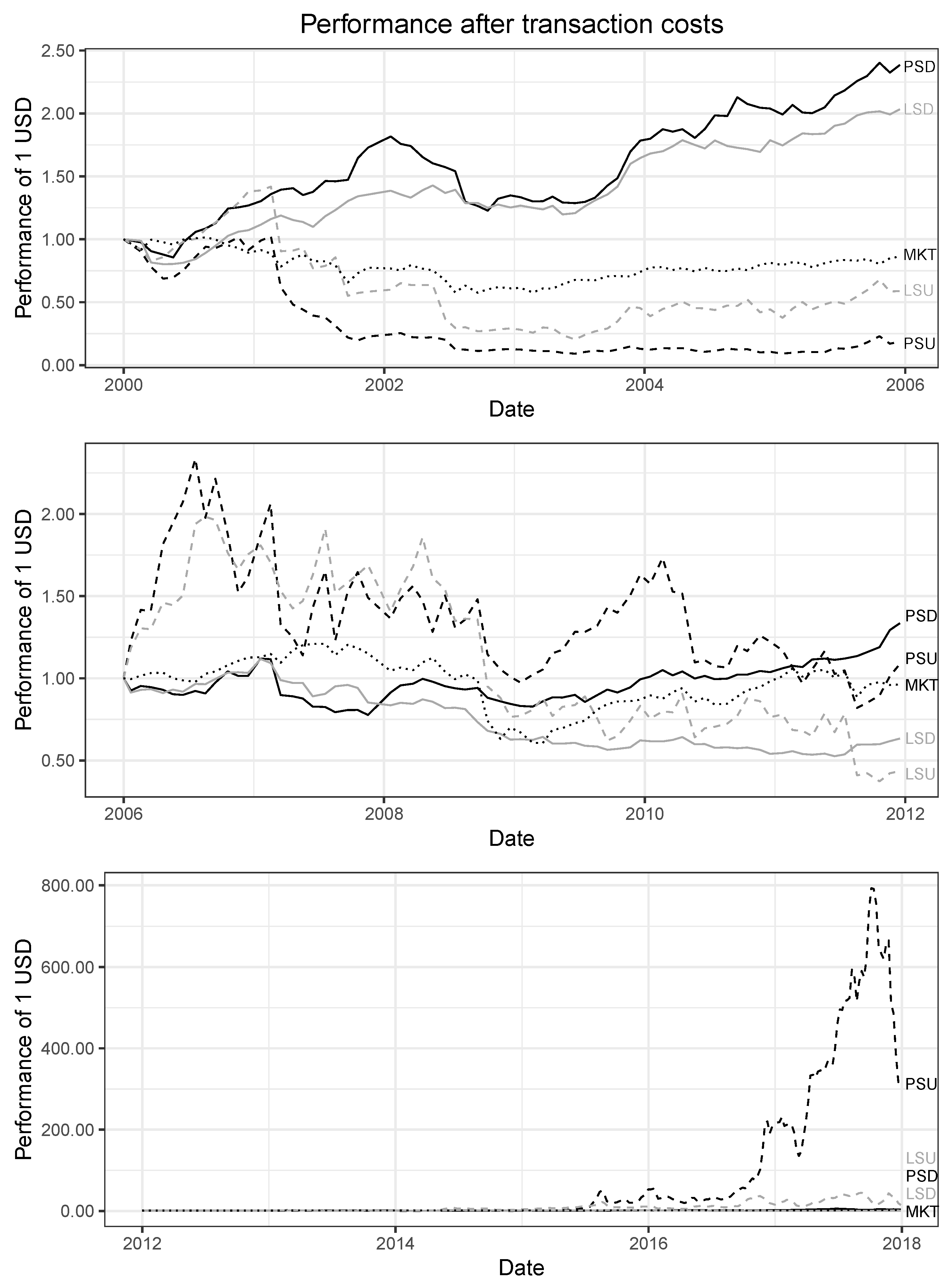
• PCA straddle delta hedged (PSD): The replicating portfolio of this strategy consists of the top five stocks that are selected with the statistical approach outlined in Section 3.2. A long straddle position of the basket portfolio is established while index straddles are sold. The overall position is delta hedged on a daily basis.
• PCA straddle delta unhedged (PSU): The selection process and the trade construction are similar to PSD. However, the directional exposure remains unhedged during the lifetime of the trade. This illustrates a simpler version of PSD.
• Largest constituents straddle delta hedged (LSD): The replicating portfolio of this strategy follows a naive subsetting approach and contains the top five largest constituents of the index at trade inception. Basket straddles are bought while index straddles are shorted. The directional exposure is delta hedged on a daily basis.
• Largest constituents straddle delta unhedged (LSU): The trade construction and selection process is identical to LSD. However, the overall delta position remains unhedged, hence representing a less sophisticated approach than LSD.
• Naive buy-and-hold strategy (MKT): This approach represents a simple buy-and-hold strategy. The index is bought in January 2000 and held during the complete back-testing period. MKT is the simplest strategy in our study.

Transaction costs are inevitable when participating in financial markets. Thus, transaction fees have to be considered in evaluating trading strategies to provide a more realistic picture of profitability. Besides market impact, bid-ask spreads, and commissions, slippages are the main cost driver. Over the last few years, trading costs decreased due to electronic trading, decimalization, increased competition, and regulatory changes (see [43,44]). The retail sector also benefited from this development as brokers such as Charles Schwab first decreased and then completely eliminated fees for stocks, ETFs, and options that are listed on U.S. or Canadian exchanges [45]. However, transaction costs are hard to estimate as they depend on multiple factors such as asset class and client profile. To account for asset specific trading fees in our back-testing study, we apply 10 bps for every half turn per option, to which $2.5$ bps are added if delta hedging is performed. In light of our trading strategy in a highly liquid equity market, the cost assumptions appear to be realistic.

3.4. Return Calculation

In contrast to [2,37,46], who constructed a fully invested portfolio, we base our returns on a partially invested portfolio. Our calculation is similar to the concept of return on risk-adjusted capital (RORAC). There are two reasons for choosing this method. First, short selling options incorporates extreme payoffs that can easily outstrip option premiums. As a result, investors need substantial liquidity to cover any future cash outflows to honor their obligations. Second, writing options requires a margin to enter and maintain the position. For example, the initial margin for a one month short index ATM call position at the Chicago Board Options Exchange (CBOE) amounts to 100% of the options proceeds plus 15% of the aggregated underlying index value minus the out-of-the-money amount [47].

The return of a dispersion trade is calculated as:

$$\begin{array}{c}\hfill R_{t,T}=\left\{\begin{array}{cccc}\hfill & {\displaystyle \frac{P_{T,Stocks}}{V_{t,Stocks}}}-{\displaystyle \frac{P_{T,Index}}{V_{t,Index}}},\hfill & \hfill & \mathrm{if}\mathrm{long}\mathrm{dispersion},\hfill \\ \hfill -& {\displaystyle \frac{P_{T,Stocks}}{V_{t,Stocks}}}+{\displaystyle \frac{P_{T,Index}}{V_{t,Index}}},\hfill & \hfill & \mathrm{if}\mathrm{short}\mathrm{dispersion},\hfill \end{array}\right.\end{array}$$

(14)

where $V_t$ represents the initial costs of the individual legs:

$$\begin{array}{cc}\hfill V_{t,Stocks}& =\sum _i^N{w}_i\left(C_{i,t}(K_i,T)+P_{i,t}(K_i,T)\right),\hfill \end{array}$$

(15)

$$\begin{array}{cc}\hfill V_{t,Index}& =C_{I,t}(K_I,T)+P_{I,t}(K_I,T).\hfill \end{array}$$

(16)

$C_t$ and $P_t$ denote the prices for calls and puts for a specific time to maturity (T) and strike (K). When delta hedging is conducted, the generated P&L is added to the nominator of Equation (14) for both legs. As [18] assumed continuous hedging is impracticable in reality due to transaction costs and a lack of order execution speed, we undertake daily delta hedging at market close. To calculate the delta exposure ($\Delta$), the Black–Scholes framework is used. $I{V}_j\forall j\in (t,T)$ is assumed to be the annualized one month trailing standard deviation of log returns. Any proceeds (losses) from delta hedging are invested (financed) at dollar LIBOR (r). This rate also serves as borrowing rate when cash is needed to buy shares (S). Hence, the delta P&L at T for a portfolio of N options is determined by:

$$\begin{array}{c}\hfill P\&L_{\Delta ,Portfolio}=\sum _{t=1}^T\sum _{i=1}^N{w}_i\left[({\Delta }_{i,t}-{\Delta }_{i,t-1})S_{i,t}*e^{r(T-t)}-{\Delta }_{i,t-1}(S_{i,t}+D_{i,t}-S_{i,t-1})\right],\end{array}$$

(17)

where $D_{i,t}$ denotes the present value at time t of the dividend payment of stock i.

4. Results

We follow [48] and conduct a fully-fledged performance evaluation on the strategies PSD, PSU, LSD, and LSU from January 2000 to December 2017—compared to the general market MKT. The key results for the options portfolio of the top five stocks are depicted in two panels—before and after transaction costs. First, we evaluate the performance of all trading strategies (Section 4.1), conduct a sub-period analysis (Section 4.2), and analyze the sensitivity to varying market frictions (Section 4.3). Second, Section 4.4 checks the robustness, and Section 4.5 examines the exposure to common systematic risk factors. Finally, we investigate the number of principal components and the corresponding sector exposure of our PCA based selection process (Section 5).

4.1. Strategy Performance

Table 3. Return characteristics, risk metrics, and trading statistics per trade for PCA straddle delta hedged (PSD), PCA straddle delta unhedged (PSU), largest constituents straddle delta hedged (LSD), and largest constituents straddle delta unhedged (LSU) from January 2000 until December 2017. NW denotes Newey–West standard errors and CVaR the conditional value at risk.

	Before Transaction Costs					After Transaction Costs
	PSD	PSU	LSD	LSU	MKT	PSD	PSU	LSD	LSU	MKT
Mean return	0.0100	0.0228	0.0044	0.0140	0.0022	0.0084	0.0214	0.0030	0.0128	0.0022
t-statistic (NW)	2.2413	2.2086	0.8608	1.5083	1.2897	1.9069	2.0933	0.5809	1.3852	1.2897
Standard error (NW)	0.0044	0.0103	0.0051	0.0093	0.0017	0.0044	0.0102	0.0051	0.0093	0.0017
Minimum	−0.2560	−0.4539	−0.2399	−0.4798	−0.2506	−0.2556	−0.4529	−0.2396	−0.4781	−0.2506
Quartile 1	−0.0238	−0.0640	−0.0288	−0.0704	−0.0097	−0.0251	−0.0648	−0.0300	−0.0711	−0.0097
Median	0.0097	0.0163	0.0037	0.0201	0.0037	0.0082	0.0150	0.0022	0.0188	0.0037
Quartile 3	0.0489	0.1006	0.0374	0.0884	0.0170	0.0470	0.0988	0.0356	0.0866	0.0170
Maximum	0.3241	1.1694	0.3414	0.4270	0.1315	0.3202	1.1626	0.3373	0.4258	0.1315
Standard deviation	0.0678	0.1523	0.0730	0.1361	0.0363	0.0673	0.1515	0.0725	0.1353	0.0363
Skewness	−0.0818	1.2340	0.2528	−0.1259	−1.5218	−0.0806	1.2366	0.2546	−0.1249	−1.5218
Kurtosis	2.7042	8.9553	2.3025	0.9795	9.2676	2.7051	8.9824	2.3021	0.9806	9.2676
Historical VaR 1%	−0.1955	−0.3580	−0.1820	−0.3584	−0.1431	−0.1955	−0.3570	−0.1820	−0.3574	−0.1431
Historical CVaR 1%	−0.2166	−0.4080	−0.2133	−0.4068	−0.1788	−0.2165	−0.4069	−0.2132	−0.4056	−0.1788
Historical VaR 5%	−0.1106	−0.2091	−0.1178	−0.2052	−0.0486	−0.1113	−0.2090	−0.1184	−0.2051	−0.0486
Historical CVaR 5%	−0.1573	−0.2889	−0.1632	−0.2977	−0.1000	−0.1576	−0.2884	−0.1635	−0.2971	−0.1000
Maximum drawdown	0.6731	0.9358	0.8074	0.8534	0.4990	0.7053	0.9470	0.8201	0.8564	0.4990
Trades with return ≥ 0	0.5747	0.5519	0.5342	0.5671	0.5975	0.5671	0.5468	0.5215	0.5646	0.5975
Number of trades	395	395	395	395	1	395	395	395	395	1
Avg. trades per year	21.9444	21.9444	21.9444	21.9444	0.0556	21.9444	21.9444	21.9444	21.9444	0.0556

Source: authors’ calculations.

shows the risk-return metrics per trade and the corresponding tradings statistics for the top five stocks per strategy from January 2000 to December 2017. We observe statistically significant returns for PSD and PSU, with Newey–West (NW) t-statistics above 2.20 before transaction costs and above 1.90 after transaction costs. A similar pattern also emerges from the economic perspective: the mean return per trade is well above zero percent for PSD (0.84 percent) and PSU (2.14 percent) after transaction costs. In contrast, LSD produces a relatively small average return of 0.30 percent per trade. It is very interesting that LSU achieves 1.28 percent, but this is not statistically significant. The naive buy-and-hold strategy MKT achieves identical results before and after transaction costs because the one-off fees are negligible. The range, i.e., the difference of maximum and minimum, is substantially lower for the delta hedged strategies PSD and LSD, which reflects the lower directional risk of those approaches. Furthermore, the standard deviation of PSU (15.23 percent) and LSU (13.53 percent) is approximately two times higher than that of PSD (6.78 percent) and LSD (7.25 percent). We follow [49] and report the historical value at risk (VaR) figures. Overall, the tail risk of the delta hedged strategies is greatly reduced, e.g., the historical VaR 5% after transaction costs for PSD is −11.13 percent compared to −20.90 percent for PSU. The decline from a historical peak, called maximum drawdown, is at a relatively low level for PSD (70.53 percent) compared to PSU (94.70 percent), LSD (82.01 percent), and LSU (85.64 percent). The hit rate, i.e., the number of trades with a positive return, varies between 52.15 percent (LSD) and 56.71 percent (PSD). Across all systems, the number of actually executed trades is 395 since none of the strategies suffers a total loss. Consequently, the average number of trades per year is approximately 22; this number is well in line with [50].

In

Table 4. Annualized risk-return measures for PSD, PSU, LSD, and LSU from January 2000 until December 2017.

	Before Transaction Costs					After Transaction Costs
	PSD	PSU	LSD	LSU	MKT	PSD	PSU	LSD	LSU	MKT
Mean return	0.1841	0.2988	0.0401	0.1049	0.0347	0.1452	0.2651	0.0077	0.0779	0.0347
Mean excess return	0.1646	0.2794	0.0206	0.0854	0.0152	0.1257	0.2456	−0.0117	0.0585	0.0152
Standard deviation	0.3192	0.7169	0.3438	0.6403	0.1710	0.3169	0.7128	0.3414	0.6367	0.1710
Downside deviation	0.2074	0.4110	0.2271	0.4264	0.1305	0.2090	0.4114	0.2287	0.4266	0.1305
Sharpe ratio	0.5157	0.3897	0.0599	0.1334	0.0890	0.3967	0.3446	−0.0344	0.0918	0.0890
Sortino ratio	2.3481	2.0620	0.4254	0.6190	0.6389	1.7935	1.7911	0.0799	0.4518	0.6389

Source: authors’ calculations.

, we report annualized risk-return measures for the strategies PSD, PSU, LSD, and LSU. The mean return after transaction costs ranges from 0.77 percent for LSD to 26.51 percent for PSU. As anticipated from Table 3, the standard deviation of both delta hedged strategies amounts to approximately 20%—half of the unhedged counterparts. Notably, the Sharpe ratio, i.e., the excess return per unit of standard deviation, of PSD clearly outperforms the benchmarks with a value of 0.40 after transaction costs. Concluding, PSD generates promising risk-return characteristics, even after transaction costs.

4.2. Sub-Period Analysis

Investors are concerned about the stability of the results, potential drawdowns, and the behavior in high market turmoils. Inspired by the time-varying returns of [51,52,53], we analyze the performance of our implemented trading strategies over the complete sample period. Figure 3 illustrates the different dispersion structures across the three different sub-periods January 2000–December 2005, January 2006–December 2011, and January 2012–December 2017. The graphs show the development of an investment of 1 USD at the beginning of each sub-period.

The first sub-period ranges from 2000 to 2005 and includes the dot-com crash, the 9/11 attacks, and the time of moderation. For PSD and LSD, 1 USD invested in January 2000 grows to more than 2.00 USD at the end of this time range; both show a steady growth without any substantial drawdowns. PSU, LSU, and MKT exhibit a similar behavior, which is clearly worse than the hedged strategies. The second sub-period ranges from 2006 to 2011 and describes the global financial crisis and its aftermath. The strategy PSD seems to be robust against any external effects since it copes with the global financial crisis in a convincing way. As expected, the unhedged trading approaches PSU and LSU show strong swings during high market turmoils. The third sub-period ranges from 2012 to 2017 and specifies the period of regeneration and comebacks. The development of all strategies does not decline even after transaction costs; profits are not being arbitraged away. Especially PSU outperforms in this time range with a cumulative return up to 300 as a consequence of too high index option premiums and high profits on single stock options, e.g., Goldman Sachs Group, Inc. and United Rentals, Inc.

4.3. Market Frictions

This subsection evaluates the robustness of our trading strategies in light of market frictions. Following [54], we analyze the annualized mean return and Sharpe ratio for varying transaction cost levels (see

Table 5. Annualized mean return and Sharpe ratio for PSD, PSU, LSD, and LSU from January 2000 until December 2017 for different transaction costs per trade per straddle in bps.

		Annualized Return					Sharpe Ratio
		PSD	PSU	LSD	LSU	MKT	PSD	PSU	LSD	LSU	MKT
Transaction costs	0	0.1841	0.2988	0.0401	0.1049	0.0347	0.5157	0.3897	0.0599	0.1334	0.0890
	1	0.1802	0.2954	0.0368	0.1022	0.0347	0.5037	0.3851	0.0504	0.1292	0.0890
	5	0.1645	0.2818	0.0238	0.0913	0.0347	0.4560	0.3670	0.0126	0.1126	0.0890
	10	0.1452	0.2651	0.0077	0.0779	0.0347	0.3967	0.3446	−0.0344	0.0918	0.0890
	15	0.1262	0.2485	−0.0080	0.0647	0.0347	0.3380	0.3222	−0.0809	0.0712	0.0890
	20	0.1075	0.2321	−0.0236	0.0516	0.0347	0.2798	0.3001	−0.1271	0.0508	0.0890
	40	0.0356	0.1687	−0.0836	0.0007	0.0347	0.0521	0.2130	−0.3082	−0.0299	0.0890
	50	0.0014	0.1381	−0.1122	−0.0238	0.0347	−0.0589	0.1703	−0.3967	−0.0696	0.0890
	60	−0.0318	0.1083	−0.1400	−0.0478	0.0347	−0.1681	0.1283	−0.4839	−0.1088	0.0890
	90	−0.1252	0.0232	−0.2185	−0.1166	0.0347	−0.4852	0.0054	−0.7380	−0.2238	0.0890
	100	−0.1544	−0.0038	−0.2431	−0.1384	0.0347	−0.5876	−0.0345	−0.8203	−0.2613	0.0890

Source: authors’ calculations.

). Motivated by the literature, our back-testing study supposes transaction costs of 10 bps per straddle and 2.5 bps per stock for delta hedging. The results for 0 bps and 10 bps are identical to Table 4. Due to the same trading frequencies, all strategies are similarly affected by transaction costs; the naive buy-and-hold strategy MKT is constant (see Section 4.1). Taking annualized returns into account, we observe that the breakeven point for PSD and LSU is between 40 bps and 80 bps. As expected, PSU has a higher level where costs and returns are equal; the breakeven point is around 90 bps. The additional consideration of the risk side leads to the Sharpe ratio, with the results being similar to before. As expected, the breakeven points are reached for lower transactions costs, as the Sharpe ratio is calculated on the basis of excess returns. The thresholds vary between approximately 5 bps for LSD and 90 bps for PSU. Concluding, the delta hedged strategies PSD and PSU provide promising results in the context of risk-return measures, even for investors that are exposed to different market conditions and thus higher transaction costs.

4.4. Robustness Check

As stated previously, the 20 percent reinvestment rate, the top stocks option portfolio, which is traded unconditionally on correlation, and the number of five target stocks was motivated based on the existing literature (Section 3.3). Since data snooping is an important issue in many research studies, we examine the sensitivity of our PSD results with respect to variations of these hyperparameters.

In contrast to the reinvestment rate and the number of target stocks, trading based on unconditional correlation is not a hyperparameter in our framework. However, it is beneficial to examine if changes in the entry signal lead to substantial changes in our strategy performance. In Section 2.1, the concept of measuring implied costs as average implied correlation is introduced. Based on this approach, the relative mispricing between the index and the replicating basket can be quantified. Applying Equation (7) to forecasted or historical volatility yields an average expected correlation. Comparing this metric to the implied average correlation provides insights regarding the current pricing of index options. As discussed in Section 2.1, index options trade usually richer in terms of implied volatility than the replication portfolio. However, there are times at which the opposite might be the case. Following, an investors would set up a short dispersion trade: selling the basket and buying the index. A simple trading signal can be derived from average correlation levels:

$$\begin{array}{cc}\hfill & \mathrm{Long}\mathrm{dispersion}\mathrm{if}{\overline{\rho }}_{implied}>{\overline{\rho }}_{historical,}\hfill \\ \hfill & \mathrm{Short}\mathrm{dispersion}\mathrm{if}{\overline{\rho }}_{implied}<{\overline{\rho }}_{historical.}\hfill \end{array}$$

For our robustness check, we rely on historical volatility as a baseline approach. However, more advanced statistical methods could be applied to forecast volatility and determine current pricing levels (see [55,56,57]).

Table 6. Annualized mean return, Sharpe ratio, and maximum drawdown before transaction costs for a varying number of top stocks, the amount of reinvestment, and the correlation filter from January 2000 until December 2017.

	Reinvestment	5%	10%	20%	40%	80%	100%
Mean return
Top 5	Uncond.Correlation	0.07120	0.11478	0.18411	0.23003	NA	NA
	Cond.Correlation	0.05096	0.07288	0.09532	0.03780	NA	NA
Top 10	Uncond. Correlation	0.06976	0.11226	0.18090	0.23413	−0.11755	NA
	Cond. Correlation	0.04677	0.06481	0.08092	0.02113	NA	NA
Top 20	Uncond. Correlation	0.07394	0.12131	0.20171	0.28533	0.00145	−0.59641
	Cond. Correlation	0.05318	0.07825	0.11008	0.08608	NA	NA
Sharpe ratio
Top 5	Uncond. Correlation	0.6467	0.5969	0.5157	0.3298	NA	NA
	Cond. Correlation	0.3902	0.3321	0.2361	0.0285	NA	NA
Top 10	Uncond. Correlation	0.6492	0.6004	0.5226	0.3475	−0.1109	NA
	Cond. Correlation	0.3496	0.2912	0.1976	0.0027	NA	NA
Top 20	Uncond. Correlation	0.7226	0.6774	0.6064	0.4424	−0.0150	−0.4100
	Cond. Correlation	0.4432	0.3879	0.2994	0.1101	NA	NA
Maximum drawdown
Top 5	Uncond. Correlation	0.2146	0.4017	0.6731	0.9258	1.0000	1.0000
	Cond. Correlation	0.2520	0.4943	0.8124	0.9908	1.0000	1.0000
Top 10	Uncond. Correlation	0.2363	0.4332	0.7053	0.9447	1.0000	1.0000
	Cond. Correlation	0.2898	0.5403	0.8399	0.9920	1.0000	1.0000
Top 20	Uncond. Correlation	0.2282	0.4198	0.6885	0.9294	0.9999	1.0000
	Cond. Correlation	0.2744	0.5187	0.8232	0.9897	1.0000	1.0000

Source: authors’ calculations.

reports the annualized return of PSD for a variety of replicating portfolio sizes, reinvestment rates, and correlation based entry signals. First of all, a higher reinvestment rate leads to higher annualized mean returns; concurrently, higher risk aggravates the Sharpe ratio and the maximum drawdown. We observe several total losses for reinvestment rates of 80 percent and 100 percent, which is a result of the corresponding all-or-nothing strategy. Higher annualized returns and Sharpe ratios can generally be found at lower numbers of top stocks indicating that our selection algorithm introduced in Section 3.2 is meaningful. Regarding the correlation filter, we recognize that the strategy based on conditional correlation leads to worse results than the unconditional counterpart, e.g., the annualized mean return for the top five stocks and an investment rate of 20 percent is 9.53 percent (conditional correlation) vs. 18.41 percent (unconditional correlation). Summarizing, our initial hyperparameter setting does not hit the optimum; our selection procedure identifies the right top stocks; and considering unconditional correlation has a positive impact on the trading results.

4.5. Risk Factor Analysis

Table 7. Risk factor exposure of PSD and PSU. The standard error is reported in brackets. FF3, Fama–French three factor model; SMB, small minus big capitalization stocks; HML, high minus low book-to-market stocks; RMW, robust minus weak; CMA, conservative minus aggressive.

	PSD			PSU
	FF3	FF3+2	FF5	FF3	FF3+2	FF5
Intercept	0.0075 **	0.0079 **	0.0074 **	0.0201 **	0.0222 ***	0.0219 ***
	(0.0035)	(0.0035)	(0.0035)	(0.0078)	(0.0080)	(0.0080)
Market	0.1200	0.1316	0.1517 *	0.2128	0.4157 **	0.0560
	(0.0834)	(0.0926)	(0.0909)	(0.1894)	(0.2084)	(0.2056)
SMB	0.1626	0.1736		0.1325	0.1920
	(0.1359)	(0.1374)		(0.3085)	(0.3092)
HML	0.2424 **	0.2360 **		0.0117	0.0767
	(0.1074)	(0.1146)		(0.2440)	(0.2579)
Momentum		−0.0225			0.0711
		(0.0893)			(0.2008)
Reversal		–0.0656			−0.5416 **
		(0.0968)			(0.2178)
SMB5			0.1168			0.0847
			(0.1551)			(0.3506)
HML5			0.1383			0.3636
			(0.1396)			(0.3157)
RMW5			−0.0216			−0.2720
			(0.1815)			(0.4102)
CMA5			0.2194			−0.8783
			(0.2362)			(0.5340)
$R^2$	0.0256	0.0267	0.0264	0.0050	0.0243	0.0146
Adj.$R^2$	0.0181	0.0142	0.0139	−0.0026	0.0118	0.0019
No. obs.	395	395	395	395	395	395
RMSE	0.0672	0.0674	0.0674	0.1527	0.1516	0.1523

*** p < 0.01, ** p < 0.05, * p < 0.1. Source: authors’ calculations.

evaluates the exposure of PSD and PSU after transaction costs to systematic sources of risk (see [48]). Therefore, we apply the Fama–French three factor model (FF3) and the Fama–French 5-factor model (FF5) of [58,59], and the Fama–French 3+2 factor model (FF3+2) presented by [2]. Hereby, FF3 measures the exposure to the general market, small minus big capitalization stocks (SMB), and high minus low book-to-market stocks (HML). Next, FF3+2 enlarges the first model by a momentum factor and a short-term reversal factor. Finally, FF5 extends FF3 by a factor capturing robust minus weak (RMW5) profitability and a factor capturing conservative minus aggressive (CMA5) investment behavior.

Across all three models, we observe statistically significant monthly alphas ranging between 0.74% and 0.79% for PSD and between 2.01% and 2.19% for PSU. The highest explanatory content is given for FF3+2 with adjusted $R^2$ of 0.0142 and 0.0118; probably, the momentum and reversal factor possess a high explanatory power. Not significant loadings for SMB5, HML5, RMW5, and CMA5 confirm our long–short portfolio we are constructing. Exposure to HML (PSD) and the reversal factor (PSU) underlies our selection and trading process (see Section 3).

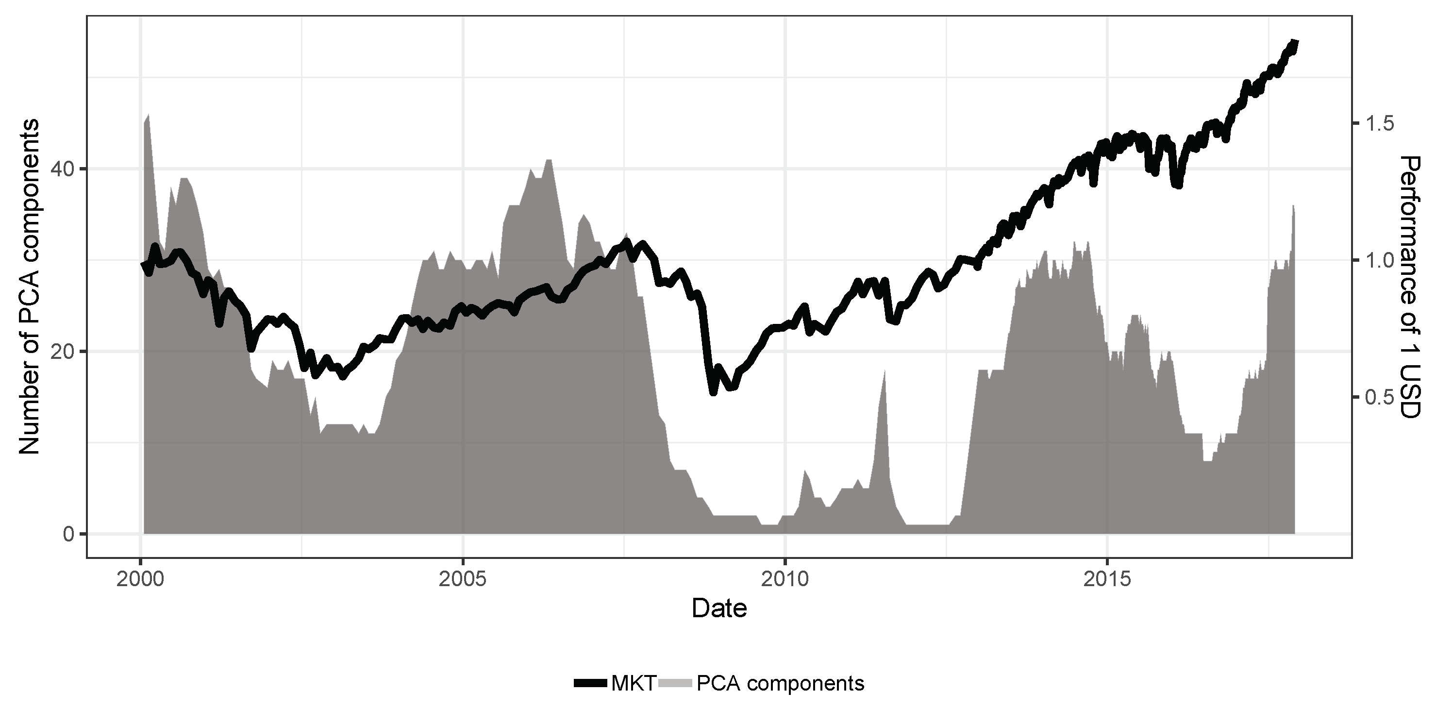
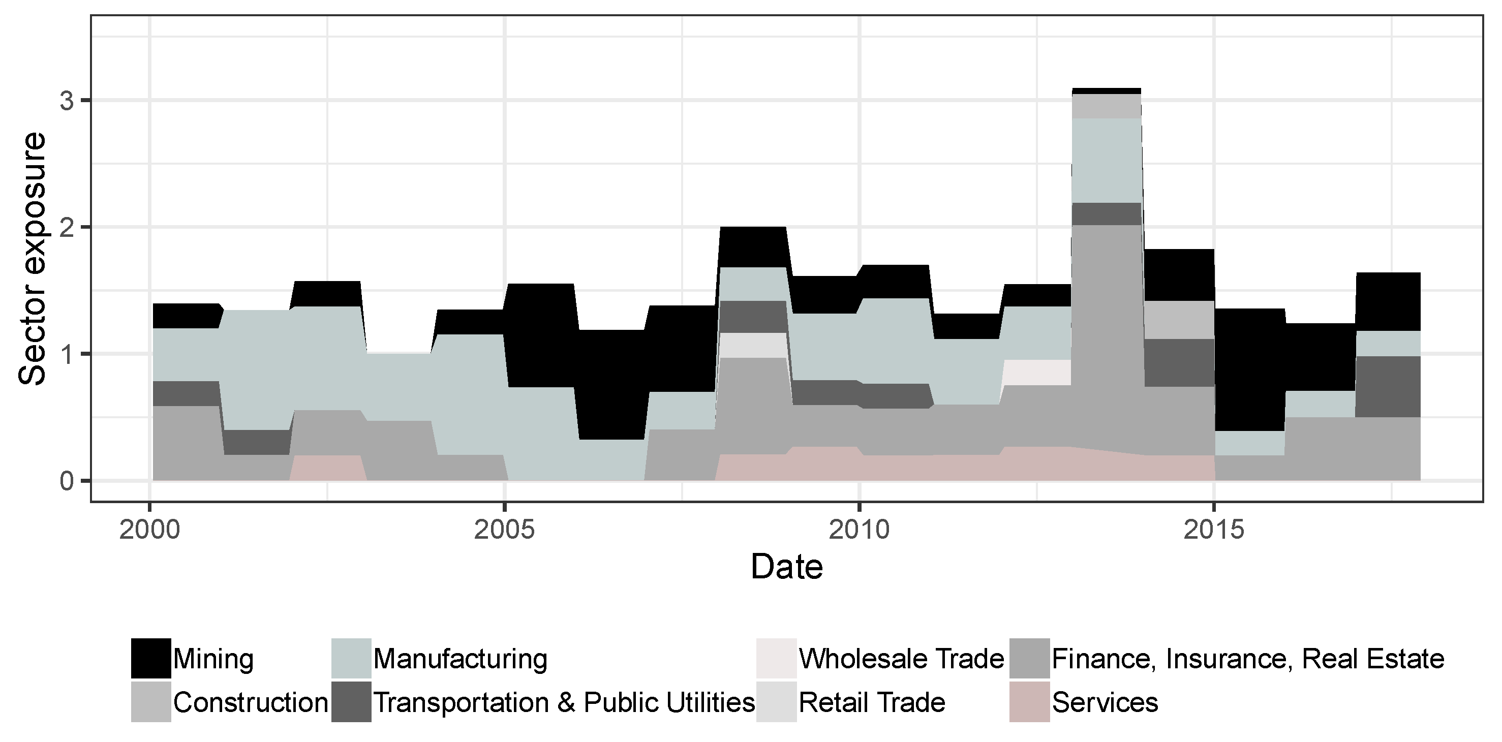
4.6. Analysis of PCA Components and Market Exposure

Following [60], we report the Kaiser–Meyer–Olkin criterion (KMO) and Bartlett’s sphericity test in

Table 8. Kaiser–Meyer–Olkin (KMO) criterion and Bartlett’s sphericity test results. The KMO values and p-values of Bartlett’s test are segmented into six and three buckets, respectively.

	Kaiser-Meyer-Olkin Criterion						Bartlett’s Sphericity Test
	KMO Value						p-Value
Segment	0–0.1	0.1–0.2	0.2–0.3	0.3–0.5	≥ 0.5	Total	< 1%	≥ 1%	Total
Count	7	84	148	138	18	395	395	0	395
Average	0.0895	0.1600	0.2445	0.3725	0.5701	0.2833	0.0000	NA	0.0000
Median	0.0878	0.1668	0.2431	0.3530	0.5502	0.2619	0.0000	NA	0.0000

Source: authors’ calculations.

to examine the suitability of our data for a PCA analysis. Bartlett’s test of sphericity, which tests the hypothesis that the correlation matrix is an identity matrix and therefore the variables are unrelated to each other and not suitable to detect any structure, is for all of our trading dates at a significance level of $1\%$ [61]. KMO is a sampling adequacy measure that describes the proportion of variance in the variables that might be caused by shared underlying factors [62,63]. A low KMO score is driven by high partial correlation in the underlying data. The threshold for an acceptable sampling adequacy for a factor analysis is normally considered to be $0.5$ [64]. However, in our context of finding the top five stocks that describe the index as closely as possible, a low KMO value is actually favorable as it indicates that strong relationships amongst the S&P 500 constituents exist that we aim to exploit with our methodology. As expected, our KMO values are on almost all trading days below the threshold with an average and median of $0.2833$ and $0.2619$, respectively. There are two determinants that explain the low KMO values in our study and support our approach. (i) Stocks are often dependent on the same risk factors, one of the most prominent factors being the market (for more, see [65,66]), and therefore exhibit rather high partial correlations. (ii) On every trading day, we analyze around 450 S&P 500 index members, which results in 101,250 different partial correlations. Due to the substantial number of combinations, you will find structure and high partial correlations in the data.

Figure 4 reports the number of required principal components to explain 90 percent of the S&P 500 constituents’ return variation and the standardized S&P 500 index. Overall, we observe synchronous developments of both time series, i.e., if one variable increases, the other increases, and vice versa. Specifically, the number of PCA components ranges between 15 and 45 from 2000 until 2007. The value decreases to approximately five with the beginning of the financial crisis in 2008. This fact is not surprising since downsides of the S&P 500 lead to a higher pair-wise correlation of the stock constituents. Consequently, a lower number of shares is in a position to describe 90 percent of stock price variations. After 2011, the general market possesses a positive trend without any strong swings. Thus, the number of PCA components increases to approximately 20.

Last, but not least, Figure 5 shows the yearly sector exposure based on our PCA selection process from January 2000 to December 2017. In line with the Standard Industrial Classification, all companies are categorized into the following nine economic sectors: “Mining”, “Manufacturing”, “Wholesale Trade”, “Finance, Insurance, Real Estate”, “Construction”, “Transportation and Public Utilities”, “Real Trade”, “Services”. Each point on the horizontal axis refers to the sectors that are used in the year after to the respective point. First of all, we observe that the sum of positive sector exposures increases in times of high market turmoil. Especially, the cumulative value exceeds three in 2013 because of a high exposure in “Finance, Insurance, Real Estate”, especially for Bank of America Corporation and Goldman Sachs Group, Inc. Furthermore, the exposure of each sector varies over time, i.e., industry branches are preferred and avoided in times of bull and bear markets. As such, the percentage of financial stocks increases in 2009 and 2013, the peak of the global financial and European debt crisis.

5. Conclusions and Policy Recommendations

In this manuscript, we developed a dispersion trading strategy based on a statistical stock selection process and applied our approach to the S&P 500 index and its constituents from January 2000 to December 2017. We contributed to the existing literature in four ways. First, we developed an index subsetting procedure that considers the individual index explanatory power of stocks in the weighting scheme. Therefore, we are in a position to build a replicating option basket with as little as five securities. Second, the large-scale empirical study provides a reliable back-testing for our dispersion trades. Hence, the profitability and robustness of those relative value trades can be examined across a variety of market conditions. Third, we analyzed the added value of our strategies by benchmarking them against a naive index subsetting approach and a simple buy-and-hold strategy. The trading frameworks that employ the PCA selection process outperformed its peers with an annualized mean return of 14.52 and 26.51 percent for PSD and PSU, respectively. The fourth contribution focuses on the conducted deep dive analysis of our selection process, i.e., sector exposure and number of required principal components over time, and the robustness checks. We showed that our trading systems possess superior risk-return characteristics compared to the benchmarking dispersion strategies.

Our study reveals two main policy recommendations. First of all, our framework shows that advanced statistical methods can be utilized to determine a portfolio replicating basket and could therefore be used for sophisticated risk management. Regulatory market risk assessments of financial institutions often rely on crude approaches that stress bank’s capital requirements disproportionately to the underlying risk. However, regulators should explore the possibility of employing more advanced statistical models in their risk assessments, such as considering PCA built replicating baskets to hedge index exposures, to adequately reflect risk. Finally, investors should be aware that a principal component analysis can be used to cost-efficiently set up dispersion trades, and they should use their comprehensive datasets to improve the stock selection process further.

For future research endeavors, we identify the following three areas. First, the back-testing framework should be applied to other indices and geographical areas, i.e., price weighted equity markets and emerging economies, to shed light on any idiosyncrasies related to geographical or index construction differences. Second, efforts could be undertaken to improve the correlation filter from Section 4.4, so that profitable short dispersion opportunities can be spotted more accurately. Third, financial product innovations in a dispersion context should be subject to future studies, particularly the third generation of volatility derivatives such as variance, correlation, and gamma swaps.

References

1. Pole, A. Statistical Arbitrage: Algorithmic Trading Insights and Techniques; John Wiley & Sons: Hoboken, NJ, USA, 2011. [Google Scholar]
2. Gatev, E.; Goetzmann, W.N.; Rouwenhorst, K.G. Pairs trading: Performance of a relative-value arbitrage rule. Rev. Financ. Stud. 2006, 19, 797–827. [Google Scholar] [CrossRef] [Green Version]
3. Do, B.; Faff, R. Does simple pairs trading still work? Financ. Anal. J. 2010, 66, 83–95. [Google Scholar] [CrossRef]
4. Ramos-Requena, J.; Trinidad-Segovia, J.; Sánchez-Granero, M. Introducing Hurst exponent in pair trading. Phys. Stat. Mech. Its Appl. 2017, 488, 39–45. [Google Scholar] [CrossRef]
5. Ramos-Requena, J.P.; Trinidad-Segovia, J.E.; Sánchez-Granero, M.Á. Some notes on the formation of a pair in pairs trading. Mathematics 2020, 8, 348. [Google Scholar] [CrossRef] [Green Version]
6. Sánchez-Granero, M.; Balladares, K.; Ramos-Requena, J.; Trinidad-Segovia, J. Testing the efficient market hypothesis in Latin American stock markets. Phys. Stat. Mech. Its Appl. 2020, 540, 123082. [Google Scholar] [CrossRef]
7. Bennett, C. Trading Volatility: Trading Volatility, Correlation, Term Structure and Skew; CreateSpace: Charleston, SC, USA, 2014. [Google Scholar]
8. Nasekin, S.; Härdle, W.K. Model-driven statistical arbitrage on LETF option markets. Quant. Financ. 2019, 19, 1817–1837. [Google Scholar] [CrossRef]
9. Glasserman, P.; He, P. Buy rough, sell smooth. Quant. Financ. 2020, 20, 363–378. [Google Scholar] [CrossRef]
10. Gangahar, A. Smart Money on Dispersion. Financial Times. 2006. Available online: https://www.ft.com/content/a786ce1e-3140-11db-b953-0000779e2340 (accessed on 16 August 2020).
11. Sculptor Capital Management Inc. Sculptor Capital Management Inc. website. 2020. Available online: https://www.sculptor.com/ (accessed on 16 August 2020).
12. Alloway, T. A $12bn Dispersion Trade. Financial Times. 2011. Available online: https://ftalphaville.ft.com/2011/06/17/597511/a-12bn-dispersion-trade/ (accessed on 16 August 2020).
13. Marshall, C.M. Dispersion trading: Empirical evidence from U.S. options markets. Glob. Financ. J. 2009, 20, 289–301. [Google Scholar] [CrossRef]
14. Maze, S. Dispersion trading in south africa: An analysis of profitability and a strategy comparison. SSRN Electron. J. 2012. [Google Scholar] [CrossRef]
15. Ferrari, P.; Poy, G.; Abate, G. Dispersion trading: An empirical analysis on the S&P 100 options. Invest. Manag. Financ. Innov. 2019, 16, 178–188. [Google Scholar]
16. Deng, Q. Volatility dispersion trading. SSRN Electron. J. 2008. [Google Scholar] [CrossRef]
17. Wilmott, P. Paul Wilmott Introduces Quantitative Finance, 2nd ed.; John Wiley: Chichester, UK, 2008. [Google Scholar]
18. Black, F.; Scholes, M. The pricing of options and corporate liabilities. J. Political Econ. 1973, 81, 637–654. [Google Scholar] [CrossRef] [Green Version]
19. Jiang, X. Return dispersion and expected returns. Financ. Mark. Portf. Manag. 2010, 24, 107–135. [Google Scholar] [CrossRef]
20. Chichernea, S.C.; Holder, A.D.; Petkevich, A. Does return dispersion explain the accrual and investment anomalies? J. Account. Econ. 2015, 60, 133–148. [Google Scholar] [CrossRef]
21. Andersen, T.G.; Bollerslev, T. Answering the skeptics: Yes, standard volatility models do provide accurate forecasts. Int. Econ. Rev. 1998, 39, 885. [Google Scholar] [CrossRef]
22. Andersen, T.G.; Bollerslev, T.; Diebold, F.X.; Labys, P. The distribution of realized exchange rate volatility. J. Am. Stat. Assoc. 2001, 96, 42–55. [Google Scholar] [CrossRef]
23. Barndorff-Nielsen, O.E.; Shephard, N. Estimating quadratic variation using realized variance. J. Appl. Econom. 2002, 17, 457–477. [Google Scholar] [CrossRef] [Green Version]
24. Markowitz, H. Portfolio selection. J. Financ. 1952, 7, 77. [Google Scholar]
25. Driessen, J.; Maenhout, P.J.; Vilkov, G. Option-implied correlations and the price of correlation risk. SSRN Electron. J. 2013. [Google Scholar] [CrossRef]
26. Faria, G.; Kosowski, R.; Wang, T. The correlation risk premium: International evidence. SSRN Electron. J. 2018. [Google Scholar] [CrossRef]
27. Bollen, N.P.B.; Whaley, R.E. Does net buying pressure affect the shape of implied volatility functions? J. Financ. 2004, 59, 711–753. [Google Scholar] [CrossRef]
28. Shiu, Y.M.; Pan, G.G.; Lin, S.H.; Wu, T.C. Impact of net buying pressure on changes in implied volatility: Before and after the onset of the subprime crisis. J. Deriv. 2010, 17, 54–66. [Google Scholar] [CrossRef]
29. Ruan, X.; Zhang, J.E. The economics of the financial market for volatility trading. J. Financ. Mark. 2020, 100556. [Google Scholar] [CrossRef]
30. Bakshi, G.; Kapadia, N. Delta-hedged gains and the negative market volatility risk premium. Rev. Financ. Stud. 2003, 16, 527–566. [Google Scholar] [CrossRef]
31. Ilmanen, A. Do financial markets reward buying or selling insurance and lottery tickets? Financ. Anal. J. 2012, 68, 26–36. [Google Scholar] [CrossRef]
32. Gatheral, J. The Volatility Surface: A Practitioner’s Guide; John Wiley & Sons, Inc.: Hoboken, NJ, USA, 2006. [Google Scholar]
33. Crépey, S. Delta-hedging vega risk? Quant. Financ. 2004, 4, 559–579. [Google Scholar] [CrossRef]
34. Jegadeesh, N.; Titman, S. Returns to buying winners and selling losers: Implications for stock market efficiency. J. Financ. 1993, 48, 65–91. [Google Scholar] [CrossRef]
35. R Core Team. Stats: A Language and Environment for Statistical Computing; R Core Team: Vienna, Austria, 2019. [Google Scholar]
36. Do, B.; Faff, R. Are pairs trading profits robust to trading costs? J. Financ. Res. 2012, 35, 261–287. [Google Scholar] [CrossRef]
37. Stübinger, J.; Schneider, L. Statistical arbitrage with mean-reverting overnight price gaps on high-frequency data of the S&P 500. J. Risk Financ. Manag. 2019, 12, 51. [Google Scholar]
38. Korajczyk, R.A.; Sadka, R. Are momentum profits robust to trading costs? J. Financ. 2004, 59, 1039–1082. [Google Scholar] [CrossRef]
39. Wold, S.; Esbensen, K.; Geladi, P. Principal component analysis. Chemom. Intell. Lab. Syst. 1987, 2, 37–52. [Google Scholar] [CrossRef]
40. Abdi, H.; Williams, L.J. Principal component analysis. Wiley Interdiscip. Rev. Comput. Stat. 2010, 2, 433–459. [Google Scholar] [CrossRef]
41. Su, X. Hedging Basket Options by Using A Subset of Underlying Assets (Working Paper). 2006. Available online: https://www.econstor.eu/bitstream/10419/22959/1/bgse14_2006.pdf (accessed on 16 August 2020).
42. von Beschwitz, B.; Massa, M. Biased short: Short sellers’ disposition effect and limits to arbitrage. J. Financ. Mark. 2020, 49, 100512. [Google Scholar] [CrossRef]
43. Voya Investment Management. The Impact of Equity Market Fragmentation and Dark Pools on Trading and Alpha Generation. 2016. Available online: https://investments.voya.com (accessed on 16 August 2020).
44. Frazzini, A.; Israel, R.; Moskowitz, T.J. Trading costs. SSRN Electron. J. 2018. [Google Scholar] [CrossRef]
45. Henderson, R. Schwab Opens New front in Trading War by Slashing Rates to Zero. Financial Times. 2019. Available online: https://www.ft.com/content/cf644610-e45a-11e9-9743-db5a370481bc (accessed on 16 August 2020).
46. Avellaneda, M.; Lee, J.H. Statistical arbitrage in the US equities market. Quant. Financ. 2010, 10, 761–782. [Google Scholar] [CrossRef] [Green Version]
47. Cboe Global Markets, I. Chicago Board Options Exchange Margin Manual. 2000. Available online: https://www.cboe.com/learncenter/pdf/margin2-00.pdf (accessed on 16 August 2020).
48. Stübinger, J.; Endres, S. Pairs trading with a mean-reverting jump-diffusion model on high-frequency data. Quant. Financ. 2018, 18, 1735–1751. [Google Scholar] [CrossRef] [Green Version]
49. Mina, J.; Xiao, J.Y. Return to RiskMetrics: The evolution of a standard. Riskmetrics Group 2001, 1, 1–11. [Google Scholar]
50. Stübinger, J.; Mangold, B.; Krauss, C. Statistical arbitrage with vine copulas. Quant. Financ. 2018, 18, 1831–1849. [Google Scholar] [CrossRef] [Green Version]
51. Liu, B.; Chang, L.B.; Geman, H. Intraday pairs trading strategies on high frequency data: The case of oil companies. Quant. Financ. 2017, 17, 87–100. [Google Scholar] [CrossRef] [Green Version]
52. Knoll, J.; Stübinger, J.; Grottke, M. Exploiting social media with higher-order factorization machines: Statistical arbitrage on high-frequency data of the S&P 500. Quant. Financ. 2019, 19, 571–585. [Google Scholar]
53. Stübinger, J. Statistical arbitrage with optimal causal paths on high-frequency data of the S&P 500. Quant. Financ. 2019, 19, 921–935. [Google Scholar]
54. Endres, S.; Stübinger, J. Regime-switching modeling of high-frequency stock returns with Lévy jumps. Quant. Financ. 2019, 19, 1727–1740. [Google Scholar] [CrossRef] [Green Version]
55. Degiannakis, S.; Filis, G.; Hassani, H. Forecasting global stock market implied volatility indices. J. Empir. Financ. 2018, 46, 111–129. [Google Scholar] [CrossRef] [Green Version]
56. Fang, T.; Lee, T.H.; Su, Z. Predicting the long-term stock market volatility: A GARCH-MIDAS model with variable selection. J. Empir. Financ. 2020, 58, 36–49. [Google Scholar] [CrossRef]
57. Naimy, V.; Montero, J.M.; El Khoury, R.; Maalouf, N. Market volatility of the three most powerful military countries during their intervention in the Syrian War. Mathematics 2020, 8, 834. [Google Scholar] [CrossRef]
58. Fama, E.F.; French, K.R. Multifactor explanations of asset pricing anomalies. J. Financ. 1996, 51, 55–84. [Google Scholar] [CrossRef]
59. Fama, E.F.; French, K.R. A five-factor asset pricing model. J. Financ. Econ. 2015, 116, 1–22. [Google Scholar] [CrossRef] [Green Version]
60. Yoshino, N.; Taghizadeh-Hesary, F. Analysis of credit ratings for small and medium-sized enterprises: Evidence from Asia. Asian Dev. Rev. 2015, 32, 18–37. [Google Scholar] [CrossRef]
61. Bartlett, M.S. The effect of standardization on a χ2 approximation in factor analysis. Biometrika 1951, 38, 337–344. [Google Scholar] [CrossRef]
62. Kaiser, H.F. A second generation little jiffy. Psychometrika 1970, 35, 401–415. [Google Scholar] [CrossRef]
63. Kaiser, H. An index of factorial simplicity. Psychometrika 1974, 39, 31–36. [Google Scholar] [CrossRef]
64. Kaiser, H.F.; Rice, J. Little jiffy, Mark Iv. Educ. Psychol. Meas. 1974, 34, 111–117. [Google Scholar] [CrossRef]
65. Sharpe, W.F. Capital asset prices: A theory of market equilibrium under conditions of risk. J. Financ. 1964, 19, 425–442. [Google Scholar]
66. Lintner, J. The valuation of risk assets and the selection of risky investments in stock portfolios and capital budgets. Rev. Econ. Stat. 1965, 47, 13–37. [Google Scholar] [CrossRef]
Figure 1. Visualization of dispersion trade performance drivers. Source: authors’ calculations.
Mathematics 08 01627 g001
Figure 2. Illustration of the effect of different correlation levels on the variance of an equally weighted index of two stocks. Source: authors’ calculations.
Mathematics 08 01627 g002
Figure 3. Development of an investment of 1 USD in PSD, PSU, LSD, and LSU after transaction costs compared to the S&P 500 (MKT). The time period is divided intro three sub-periods from January 2000–December 2005, January 2006–December 2011, and January 2012–December 2017. Source: authors’ calculations.
Mathematics 08 01627 g003
Figure 4. Number of required principal components to explain 90% of S&P 500 constituents return variation and S&P 500 index performance (MKT) from January 2000–December 2017. Source: authors’ calculations.
Mathematics 08 01627 g004
Figure 5. Yearly sector exposure based on the PCA selection process from January 2000–December 2017. Sector short positions are for illustrative purposes not included. Source: authors’ calculations.
Mathematics 08 01627 g005