Non-Parametric Analysis of Efficiency: An Application to the Pharmaceutical Industry

Abstract

Increases in the cost of research, specialization and reductions in public expenditure in health are changing the economic environment for the pharmaceutical industry. Gains in productivity and efficiency are increasingly important in order for firms to succeed in this environment. We analyze empirically the performance of efficiency in the pharmaceutical industry over the period 2010–2018. We work with microdata from a large sample of European firms of different characteristics regarding size, main activity, country of origin and other idiosyncratic features. We compute efficiency scores for the firms in the sample on a yearly basis by means of non-parametric data envelopment analysis (DEA) techniques. Basic results show a moderate average level of efficiency for the firms which encompass the sample. Efficiency is higher for companies which engage in manufacturing and distribution than for firms focusing on research and development (R&D) activities. Large firms display higher levels of efficiency than medium-size and small firms. Our estimates point to a decreasing pattern of average efficiency over the years 2010–2018. Furthermore, we explore the potential correlation of efficiency with particular aspects of the firms’ performance. Profit margins and financial solvency are positively correlated with efficiency, whereas employee costs display a negative correlation. Institutional aspects of the countries of origin also influence efficiency levels.

1. Introduction

Pharmaceutical companies contribute crucially to the health and welfare of individuals. This issue is particularly relevant nowadays: as the Covid-19 pandemic has shown, no country is immune to the emergence of new diseases. Furthermore, the population in many countries is experiencing deep demographic transformations which increase life expectancy and raise new challenges for policymakers. Not surprisingly, the performance of the industry directly affects some of the Sustainable Development Goals of the 2030 Agenda for Sustainable Development.

The economic importance of the industry is also paramount. The pharmaceutical sector employs highly skilled labor and exhibits one of the largest figures of research and development (R&D) intensity (defined as expenditure in R&D as a share of sales). As recent contributions in the field of macroeconomics have shown, human capital and R&D are key drivers of economic growth, productivity and prosperity [1,2,3].

The pharmaceutical industry is facing new challenges because of several factors. New diseases as the Covid-19 demand quick, pathbreaking solutions. R&D costs grow because conditions become chronic and more complicated. Paradoxically, the progress in molecular biology which increases the range of potential innovations also raises the complexity of decisions related to the R&D strategy. New investments seek increasingly high risk/high premium drugs [4]. Official agencies accumulate requirements for drug approvals. Firms must cope with the expiration of patents and with reductions in public expenditure in healthcare due to stability measures and fiscal adjustments.

Meanwhile the business model in the industry has experienced deep transformations over the last decades. Some firms have specialized in particular steps of the value chain, as R&D in the biotechnological sphere or clinical research, this last in the case of contract research organizations (CROs). Reductions in R&D productivity have brought about mergers and acquisitions, partly to profit from the expertise in research and the pipeline of other companies. Reference [5] argue that Japanese firms engaged in mergers and acquisitions over 1980–1997 to handle the declining productivity of R&D. Other firms outsource activities or engage in technological alliances [6,7]. In this context, firms must strive to increase their levels of productivity and efficiency, which may become a strategic asset [8].

In parallel, empirical research on productivity and efficiency (defined as output per unit of inputs) has grown over the last decades. Mathematical techniques such as data envelopment analysis (DEA) have facilitated the empirical assessment of efficiency at the country, entity or firm level. The literature has explored the levels and trends of efficiency in many activities and areas such as banking [9], farming [10], food [11], universities [12], airlines [13], shipping [14], oil [15], electricity distribution [16,17] and energy consumption [18,19], to quote just a few examples.

Recent meta-analyses and compilations of DEA exercises can be found in [20] for the public sector, [21] for energy and the environment, [22] for seaports, [23] for microfinance institutions and [24] for rail transport. [25] provide a thorough list of the main journal articles on DEA methodology and applications published between 1978 and 2016.

Researchers have also dealt with more theoretical aspects of the DEA model. Examples are [26], which describes a dynamic version of DEA that allows intertemporal links between inputs and outputs to be considered, and [27] which provides an alternative to the inverse DEA model. Furthermore, [28] explore the features of the model when the data are imprecise and [29] devise a DEA algorithm suitable to deal with Big Data.

The analysis of efficiency in the pharmaceutical industry has also been addressed in the recent past [8,30] although the number of contributions in this regard is comparatively sparse. Most of the studies in this area perform their analyses at the country level and/or focus on a (usually small) sample of companies. Examples are [31] for China; [32,33] for Japan; [6] for US; [34] for Jordan and [35] for India.

We intend to complement this literature with a two-stages analysis of efficiency within a relatively large sample of European firms. In the first stage we compute efficiency levels for the firms in our sample. In the second stage we explore by statistical modelling the connection between the efficiency scores obtained in the first stage and a set of variables potentially correlated with efficiency.

We are especially interested in the assessment of efficiency by type of activity and firm size. More specifically, we want to explore whether large firms exhibit higher levels of efficiency, which would be consistent with the potential presence of scale economies in the industry. Furthermore, it is feasible that firms which primarily operate in the R&D niche enjoy a different level of efficiency, on average, than companies with activities along the entire value chain. Finally, we want to explore the data to find common patterns and detect possible features of the economic and institutional framework and firm management strategy which can be correlated with efficiency.

In parallel, our empirical exercise may prove useful to illustrate how to apply modern mathematical, non-parametric techniques in order to get insights about the performance of firms in a particular industry, and how these tools are related to more traditional, parametric approaches.

Our paper is closely related to three DEA explorations of the pharmaceutical industry: [6,8,35].

Reference [8] analyze efficiency in a sample of 37 large firms from different countries over 2008–2013. They report an average level of efficiency in their sample of 0.9345 and find that firms with higher level of efficiency carry out more financial transactions with other companies.

We complement this exploration in several dimensions. First, our sample is different, broader and more heterogeneous, since it encompasses a large group of European firms, of different sizes and profiles. Second, we report an average efficiency score of 0.34. We think that this figure is a more accurate reflection of the mean efficiency for the whole industry, at least for the European case.

Third, we carry out a two-stage exploration of efficiency whereby in the second stage we look at variables potentially correlated with the efficiency levels obtained in the first stage. Reference [8] omit the second stage because it is somehow controversial. It is true that the literature has not reached a consensus yet on the right specification for the second stage; nonetheless, we think that this analysis can still provide some valid insights about efficiency.

Fourth, we work with a more recent time horizon, 2010–2018, and examine the dynamic performance of efficiency over time; they look at data from 2008–2013 but perform their analysis on average terms, so they do not uncover the pattern of efficiency over time.

Another related investigation is [6]. They employ proprietary data from a sample encompassed by 700 US pharmaceutical firms over the period 2001–2016. They assess the connection between open innovation methods and efficiency.

Reference [35] utilize data from a financial database to examine the performance of a group of Indian firms over the years 1991–2005. They perform a two-stage analysis. In the second stage they examine the determinants of efficiency in their sample by regression tools.

In contrast to [6,35], we work with a sample made up of European firms and explore the potential impact of alternative aspects of firm management and country characteristics. While [35] employ only a Tobit specification in the second stage of their analysis, we utilize also a pure random-effects and a Simar–Wilson procedure, and perform a comparison of the three methods.

We contribute to the literature in several ways. To the best of our knowledge, we are the first to perform a DEA analysis for a relatively large sample of European pharmaceutical firms, of different sizes and main activities, fully exploiting the time dimension of the data.

The inclusion of biotechnological companies in our sample and the exploration of their specific performance are also novel features of our investigation.

We introduce in the second stage of our empirical work a set of variables potentially correlated with efficiency, capturing different aspects of firm management and the macroeconomic environment where companies operate. Employing these variables is original as well in these kinds of analysis.

Finally, we compare the results for the second stage of three different estimation procedures (Tobit, pure random-effects, Simar–Wilson [36]). While the estimates yielded by the Tobit and the pure random-effects specifications are rather close, the Simar–Wilson tool provides larger point estimates. Nonetheless, the quantification of the marginal effects of the main covariates are more similar, and therefore the Simar–Wilson method may also be useful in applied research.

Our investigation suggests that the level of efficiency in the European pharmaceutical industry is moderate and has displayed a decreasing trend over the period 2010–2018. We find a connection between size and efficiency for the firms in our sample, where larger and very small firms tend to perform better as far as efficiency is concerned. Instead, efficiency is smaller for medium and small firms.

In terms of activity, companies operating over the complete value chain register higher levels of efficiency than firms that specialize in the R&D area. Moreover, the geographical market where firms operate seems to matter for their efficiency. Higher margins, sound financial management and lower levels of employee cost are also positively correlated with efficiency according to our results.

The structure of this paper is the following: Section 2 describes the theoretical background of our investigation. Section 3 describes the data and empirical strategy pursued. Section 4 and Section 5 discuss the main results of our analysis and Section 6 concludes.

2. Theoretical Background

Conventional microeconomic theory assumes that firms optimize by producing the maximum possible quantity of output for a given input endowment or, equivalently, by producing a given amount of output with the minimum feasible inputs; this is tantamount to presupposing that they are efficient.

Empirical evidence and casual observation suggest that this is not necessarily the case. Inefficiencies exist and may arise due to managerial practices [37] or cultural beliefs [38]. Moreover, some features of the macroeconomic environment where companies operate, as information asymmetries or market rigidities, may also be detrimental for firms’ productivity, as some important breakthroughs in macroeconomics in the last decades have pointed out.

Modern applied research pursues productivity analyses through two main avenues: stochastic frontier analysis (SFA) and DEA. While the intuition of both approaches is similar, the procedures are different.

In both cases the starting point is the idea of an efficient combination of inputs and outputs which encompasses a production function or frontier. The units of analysis are the so-called decision-making units or DMUs, i.e., the firms, organizations, institutions etc. whose efficiency is explored. The main difference between SFA and DEA lies in their methodology. SFA estimates the (continuous) production function by statistical techniques; DEA fits a piecewise hull enveloping the data which is assumed to approximate the true frontier, without making any statistical assumption about the data-generating process.

SFA originated with the pathbreaking contributions of [39,40]. In this setting, deviations from the estimated production function can be decomposed in statistical noise and inefficiency. Therefore, the error term in these models is usually composite [41].

An SFA model may be described by Equation (1)

$$\begin{gathered} y_i=m\left(x_i; \beta \right)+{ϵ}_i \\ {ϵ}_i= v_i-u_i \\ {v}_i ~ N\left(0, {\sigma }_v^2\right) \\ {u}_i ~ ℱ \end{gathered}$$

(1)

where y_i is (log) output for the ith decision-making unit or DMU, x_i is a vector of inputs for the ith DMU, ε_i the vector of parameters to be estimated, u_i captures the (one sided) inefficiency of the ith DMU and v_i represents stochastic shocks. m(.) is the production function, usually assumed to be Cobb Douglas or Translog. The estimation is ordinarily implemented by maximum likelihood or other appropriate methodologies.

The stochastic shock is usually considered normal with zero mean and known variance, whereas different distributions have been advocated and estimated in the literature for the term capturing inefficiency (for a thorough review, see [41]).

The assumption about the error term may be too restrictive. Sometimes it may be preferable to work with a more flexible specification which involves fewer hypotheses. This is why non-parametric techniques, and in particular DEA, have been developed and used increasingly in recent years.

In the applied work, nonetheless, parametric and non-parametric tools sometimes intertwine: the non-parametric approach may be complemented by some statistical analyses, usually by regression procedures, which explore the output of DEA and employ inference to generalize its results to a non-deterministic setting.

Data Envelopment Analysis

The seminal paper for DEA is [42]. This technique computes efficiency by linear programming. The technique operates in two steps: first, it constructs the frontier from the data; second, it computes the distance of each unit to the frontier. It is assumed that the DMUs with the greatest efficiency determine the frontier and have efficiency of 1.

Not all efficient DMUs, however, need to be real: they can be fictitious, i.e., linear combinations of other units. This assumes, in turn, that inputs can be used continuously, i.e., they are divisible. Moreover, it presupposes that the efficiency frontier is a convex set, and hence the linear combination of two points belonging to the feasible set are also feasible. The efficient DMUs which generate a fictitious unit are called referees.

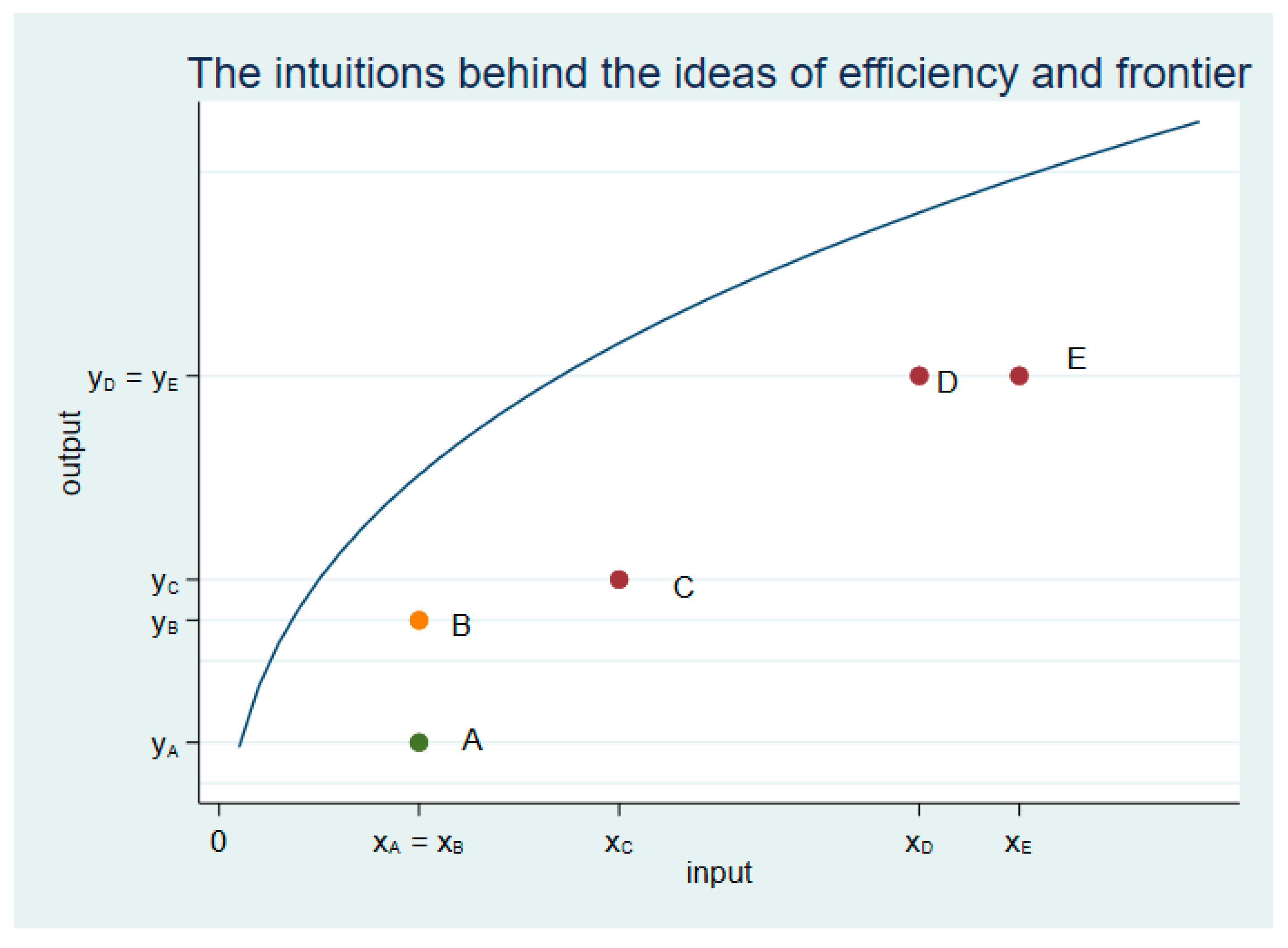
The ideas of frontier and distance encompass an intuitively appealing way to address the study of efficiency. Consider a simple example, firms from an industry which produce a single output y by means of an input x (Figure 1) (this example can be immediately generalized to the case of a vector of outputs and a vector of inputs). There are several firms or DMUs dubbed A, B, C, D, and E. The coordinates for each point in the x, y, space symbolize the input employed and the output produced by each firm. The frontier (solid line) represents optimal combinations of inputs and outputs. It is immediate to notice that B provides more output than A, y_B > y_A, while using the same amount of input since x_A = x_B. Alternatively, D and E produce the same output, y_D = y_E, but firm D consumes a smaller amount of input than E, x_D < x_E.

We say than B is more efficient than A and that D is more efficient than E. The closer a firm to the frontier, the larger its efficiency. Conversely, the deviations from the frontier can be understood as inefficiencies.

It is clear from Figure 1 that optimality can be defined in two alternative ways, maximum output per unit of input or minimal consumption of resources to attain a certain level of output. The first approach is named output oriented while the second is called input oriented.

Suppose there are N DMUs with a technology characterized by constant returns to scale. For the ith firm we can define the following ratio of outputs to inputs:

$$ratio i= \frac{{\alpha }^{\prime }{y}_i}{{\beta }^{\prime }{x}_i}$$

$$i=1, \dots , N$$

where y_i is a vector of M outputs and x_i a vector of K inputs.

The maximization of efficiency implies the following problem:

$$\underset{\alpha ,\beta }{\max } \frac{{\alpha }^{\prime }{y}_i}{{\beta }^{\prime }{x}_i}$$

subject to the following constraints:

$$\frac{{\alpha }^{\prime }{y}_s}{{\beta }^{\prime }{x}_s} \le 1, s=1,\dots , N$$

(2)

$${\alpha }_m\ge 0, m=1,\dots , M$$

(3)

$${\beta }_k\ge 0, k=1,\dots , K$$

(4)

The restriction given by Equation (2) implies that the efficiencies of all firms have to be less or equal that 1. Restrictions given by (3) and (4) rule out negative weights of outputs and inputs.

Intuitively, the problem seeks the optimal weights such that the efficiency of the firm i is maximized, while operating within the feasible set implied by the constraints.

Imposing the restriction ${\beta }^{\prime }{x}_i=1,$ this fractional programming problem can be linearized ([43]) and transformed into the following:

$$\underset{\alpha ,\beta }{\max }{\alpha }^{\prime }{y}_i$$

subject to:

$${\beta }^{\prime }{x}_i=1$$

$${\alpha }^{\prime }{y}_s-{\beta }^{\prime }{x}_s\le 0, s=1,\dots ,N$$

$$\alpha \ge 0$$

$$\beta \ge 0$$

which can be written in the envelopment form as:

$$\underset{\theta ,\lambda }{\min }{\theta }_i$$

subject to:

$${\displaystyle \sum }_{s=1}^N{\lambda }_s{y}_s-y_{i } \ge 0$$

$${\theta }_i{x}_i-{\displaystyle \sum }_{s=1}^N{\lambda }_s{x}_s \ge 0$$

$${\lambda }_s\ge 0$$

where θ_i is the input oriented efficiency score for the ith firm.

λ stands for the set of multipliers in the linear combinations of the DMUs’ inputs and outputs, i.e., the weight of each DMU within the peer group of DMUs.

This set up can also be applied to a technology exhibiting variable returns to scale by adding the convexity condition:

$${\displaystyle \sum }_{s=1}^N{\lambda }_s=1$$

This is an optimization problem, with linear objective function and constraints, solvable by linear programming.

The value of θ_i, the input-oriented technical efficiency score for the ith firm, indicates to what extent the inputs can be reduced in percent while keeping the output constant. For example, if DMU i has an efficiency score of 90%, it can reduce all inputs by 10% while offering the same amount of output.

Notice the difference between this set up and the statistical approach of SFA as presented in Equation (1) above.

The empirical exercise described in this paper employs the non-parametric, DEA formulation of the optimization problem as the baseline for analysis.

3. Material and Method: Data and Empirical Strategy

Data have been gathered primarily from Amadeus [44] a rich database comprising disaggregated economic and financial information from a large number of European companies. [8,35] employ also financial information from similar databases for their analyses.

Within the pharmaceutical industry, we have selected two main categories of firms in Amadeus according to their main activity:

(i)

Manufacture of basic pharmaceutical products and pharmaceutical preparations;

(ii)

Research and experimental development on biotechnology.

They will be labelled henceforth manufacturers and R&D firms, respectively. The two subgroups correspond to NACE (Nomenclature statistique des Activités Économiques dans la Communauté Européenne) codes 2110, 2120 (for manufacturers) and 7211 (for R&D firms). This is equivalent to NAICS (North American Industry Classification System) codes 541714 and 541715.

We work with yearly observations over the time horizon 2010–2018.

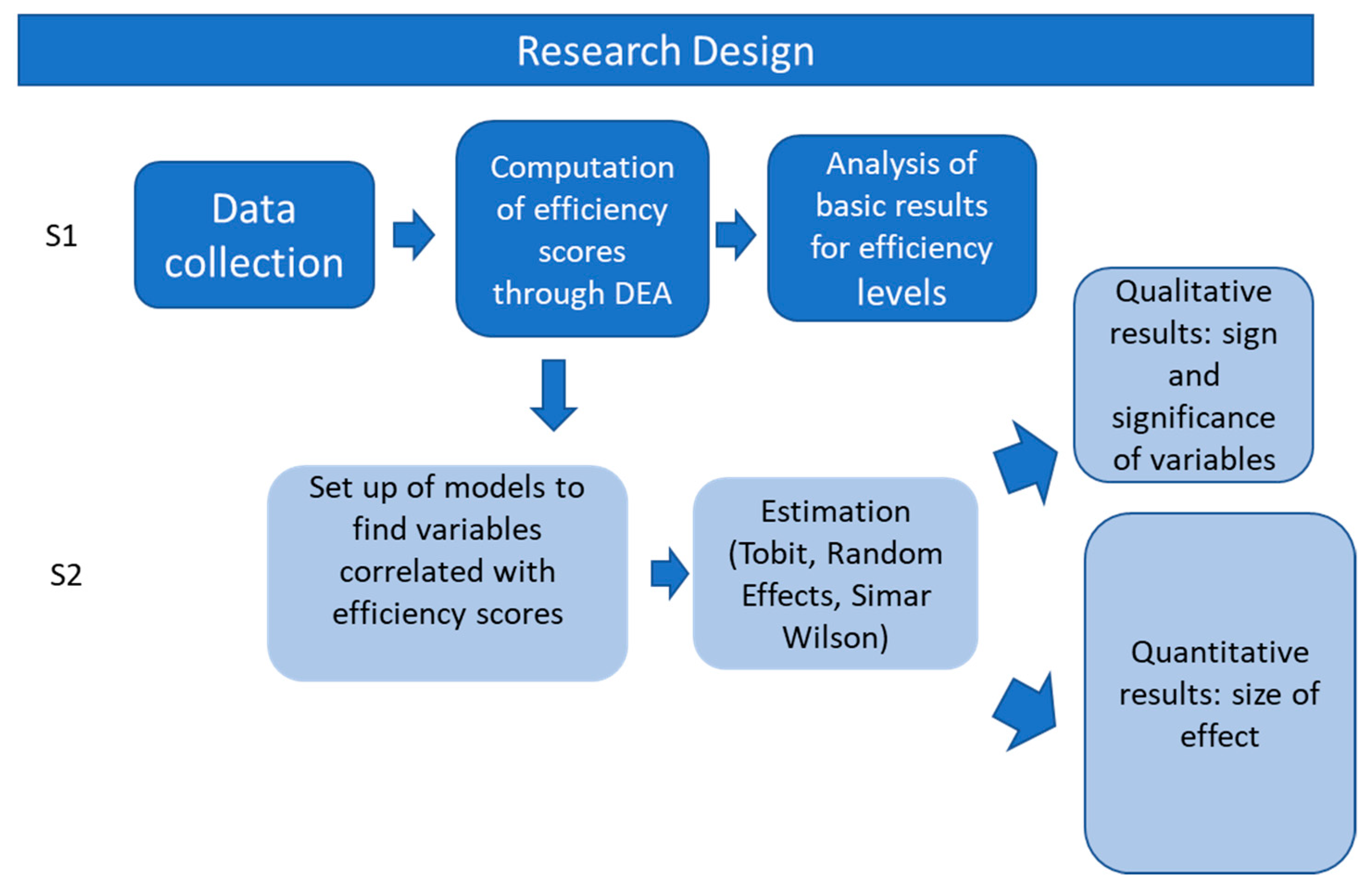
Following part of the literature on DEA, our research design has two stages (see Appendix A for an explanatory diagram of the design of our empirical exercise). The stages are detailed in Section 4 and Section 5, respectively. In the first stage we compute the efficiency scores of the firms in our sample by DEA. In the second stage we design and estimate several statistical models to explore potential variables correlated with the efficiency scores; these models provide information regarding the sign of the correlation between the efficiency score and each variable, its statistical significance and its size.

Ordinarily, non-parametric techniques cannot be applied to data structured in panels because of tractability considerations, as is common, instead, with other methodologies which allow for an explicit time dimension and have been successfully employed with panels. We circumvent this problem computing measures of efficiency year by year. This feature may be regarded as a drawback on a priori grounds; nonetheless, the estimation of efficiency measures performed on a yearly basis has been useful to uncover interesting patterns in their evolution over time.

We have started to work with a sample encompassed by more than 4000 observations from 482 firms over the nine years in the period 2010–2018, evenly split among manufacturers and R&D firms.

For the computation of efficiency for a particular year, however, we have dismissed those observations corresponding to firms which do not report data of turnover, employees and/or assets for that same year. After discarding the firms with missing values, we end up with samples comprising around 200 companies for each year, of different sizes, geographical origins and performances over time. The samples, therefore, are quite representative of the industry.

In the case of multinationals, firms correspond to headquarters. In our selection of companies we have discarded local affiliates because internal accounting procedures of multinationals may reduce their degree of comparability.

Nominal variables have been deflated using the Harmonized European Index from Eurostat [45].

Our measure of output is turnover in real terms (in constant euros of 2015). The inputs labor and capital are proxied by the number of employees and total assets in real terms, respectively. Total assets in real terms are also measured in constant euros of 2015. The choice of these variables has been made in accordance with other contributions performing similar analyses, as [6,8,32].

Economic and financial conditions have been captured by cash flow over turnover, profit margin and average cost of employees, among others (see Appendix B).

We have constructed dummies for size, country of origin, main activity and years. The specific details will be provided in Section 4 and Section 5 below.

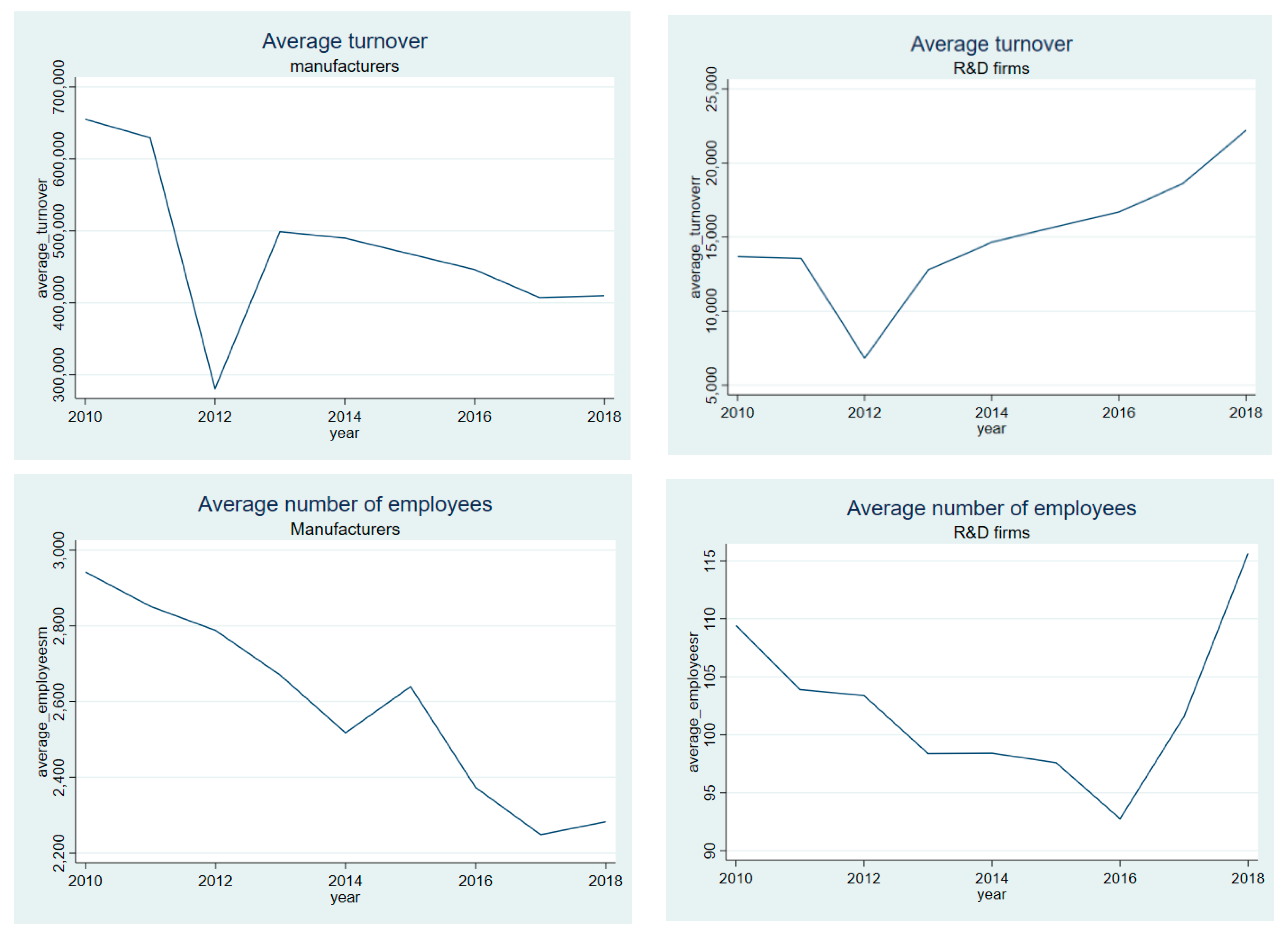
Figure 2 conveys some information for selected variables, disaggregated in manufacturers and R&D firms. Real turnover is expressed in constant euros of 2015. It is apparent from the Figure that the firms encompassing the first category are considerably larger than those in the second, as shown by the average real turnover and average number of employees.

It is also clear that both variables have experienced a decreasing pattern over time for manufacturers, with a very pronounced drop in 2012 in the case of real turnover. This is consistent with the increasingly difficult environment in which they operate. For R&D firms, the pattern is less straightforward. Average real turnover has also plummeted in 2012 but has increased thereafter. Average number of employees falls until 2016 and rises in the last years of the period.

These trends may be associated to the progressive outsourcing of some stages of the value chain, which were traditionally performed by manufacturers and now are increasingly implemented by CROs and other biotechnological firms.

Two more considerations about our empirical strategy are in order. First, and as stated above, the DEA analysis can be implemented in an output oriented or input oriented setting. We have followed this second approach since it seems intuitively more appealing and conforming with firms’ experience: their plans to increase efficiency are usually linked to reduction in costs, rather than to expansions in output.

Secondly, the relevant role played by R&D in this industry suggests that scale economies might be prevalent, but this is a controversial issue which the literature has not been able to settle yet. Reference [46] found evidence in favor of this hypothesis; Reference [47], however, did not, although they did suggest that economies of scope and accumulated knowhow were important for the firms in the sector. Reference [48] encountered knowledge spillovers among firms in Phase I of clinical research and diseconomies of scope in later phases. Reference [32] find that 60% of the firms in their sample of Japanese chemical and pharmaceutical companies operate with either increasing or decreasing returns to scale.

There is no consensus yet, therefore, on the degree of homogeneity of the production function in the industry. Anyhow, since the existence of increasing returns to scale cannot be ruled out, we have chosen to employ a variable returns to scale model as our theoretical framework, rather than a constant returns to scale. Reference [8] follow a similar approach.

4. Stage 1: Computation of Efficiency Scores

Pharmaceutical and biotechnological firms share some activities and hence compete with each other in certain stages of the value chain. We are interested in assessing whether the companies specialized in R&D activities are more or less efficient, being thus better or more poorly positioned to succeed and survive, than companies which are mainly producers and sellers. Hence, we analyze the firms in the industry jointly, i.e., with respect to an efficient frontier common for all of them (nonetheless, we have performed the analysis separately in each of the subgroups and basic results carry over).

Table 1. Efficiency in the pharma and biotechnological European industry by activity, 2010–2018.

	Efficiency Mean	Standard Deviation	Coefficient of Variation
Whole sample	0.341	0.265	0.777
Manufacturers	0.381	0.266	0.698
R&D firms	0.281	0.251	0.893

Note: the table summarizes selected statistics for efficiency levels, computed as described in the main text. We classify firms in two groups, manufacturers and R&D firms, according to their main activity. Source: Own elaboration.

,

Table 2. Relative efficiency in the pharma and biotechnological European industry by size, 2010–2018.

	Mean	Standard Deviation	Coefficient of Variation
Huge	0.98	0.039	0.039
Very big	0.765	0.205	0.267
Quite big	0.425	0.266	0.625
Medium	0.312	0.218	0.698
Small	0.267	0.19	0.71
Very Small	0.318	0.288	0.9

Note: the table summarizes selected statistics for efficiency levels, disaggregated by size of the firms (proxied by real turnover). The thresholds are described in the main text. Source: Own elaboration.

,

Table 3. Efficiency in the pharma and biotechnological European industry by activity, yearly results, 2010–2018.

	2010	2011	2012	2013	2014	2015	2016	2017	2018
Whole sample	0.428	0.392	0.348	0.308	0.304	0.292	0.383	0.311	0.334
Manufacturers	0.481	0.449	0.391	0.351	0.334	0.335	0.409	0.34	0.367
R&D firms	0.338	0.277	0.263	0.243	0.267	0.231	0.345	0.272	0.294

Note: the table details average levels of efficiency by year and main activity of firms. Efficiency is computed as described in the main text. Source: Own elaboration.

,

Table 4. Variables correlated with efficiency, Tobit estimations. Dependent variable is efficiency.

	Model 1	Model 2	Model 3	Model 4
profit_margin	0.1539 ***
	(7.00)
Germany	0.0799	0.1178 **	0.0818	0.1045 *
	(1.38)	(2.02)	(1.49)	(1.89)
Spain	−0.0232	−0.0614	0.0305	0.0435
	(0.44)	(1.10)	(0.54)	(0.87)
France	0.0100	0.0544	−0.0117	0.0167
	(0.17)	(0.94)	(0.21)	(0.31)
Sweden	0.2977 ***	0.2615 ***	0.2389 ***	0.3008 ***
	(3.93)	(3.44)	(3.45)	(4.13)
Italy	0.1421 ***	0.1549 ***	0.1587 ***	0.1374 ***
	(2.62)	(2.85)	(2.85)	(2.79)
UK	0.1389 ***	0.1637 ***	0.1128 ***	0.1356 ***
	(3.62)	(4.16)	(2.88)	(3.64)
Manufacturers	0.0660 **		0.1599 ***
	(2.00)		(4.96)
Huge	0.2054 **			0.2393 ***
	(2.49)			(3.02)
Verybig	0.1276 ***			0.1163 ***
	(3.61)			(3.24)
Quitebig	0.0215			0.0179
	(1.39)			(1.09)
year2014	−0.0795 ***	−0.0744 ***	−0.0633 ***	−0.0738 ***
	(6.90)	(6.37)	(5.88)	(6.16)
year2015	−0.1733 ***	−0.0758 ***	−0.0556 ***	−0.1537 ***
	(4.97)	(4.69)	(5.31)	(4.35)
year2016	0.0373 ***	0.0465 ***	0.0439 ***	0.0441 ***
	(3.32)	(4.12)	(4.34)	(3.79)
cash_flow		0.1650 ***
		(6.86)
Biotech		−0.1384 ***		−0.0494
		(4.21)		(1.59)
Medium		−0.0300 *
		(1.81)
Small		−0.0614 ***
		(3.22)
Verysmall		−0.0069
		(0.29)
collection_period			−0.0226 ***
			(4.44)
employee_cost				−0.3739 ***
				(10.22)
_cons	0.2808 ***	0.3788 ***	0.2245 ***	0.4390 ***
	(7.95)	(12.50)	(6.37)	(15.49)
Likelihood Ratio test of σ2u = 0: X2(1)	928.17 ***	980.9 ***	1505.81 ***	771.79 ***
Likelihood Ratio test of σ2u = 0: p value	0	0	0	0
Number observations	1547	1344	1850	1353

Notes: The table summarizes the results from the Tobit estimation of Equation (6). Dependent variable is efficiency computed in Stage 1. Cons stands for the intercept. For the rest of variables, see main text. Data are organized in a panel varying across firms and time over 2010–2018. In order to circumvent heteroskedasticity, estimations have been performed with corrected standard errors; the variance-covariance matrix of the estimators is the matrix of second derivatives of the likelihood function. 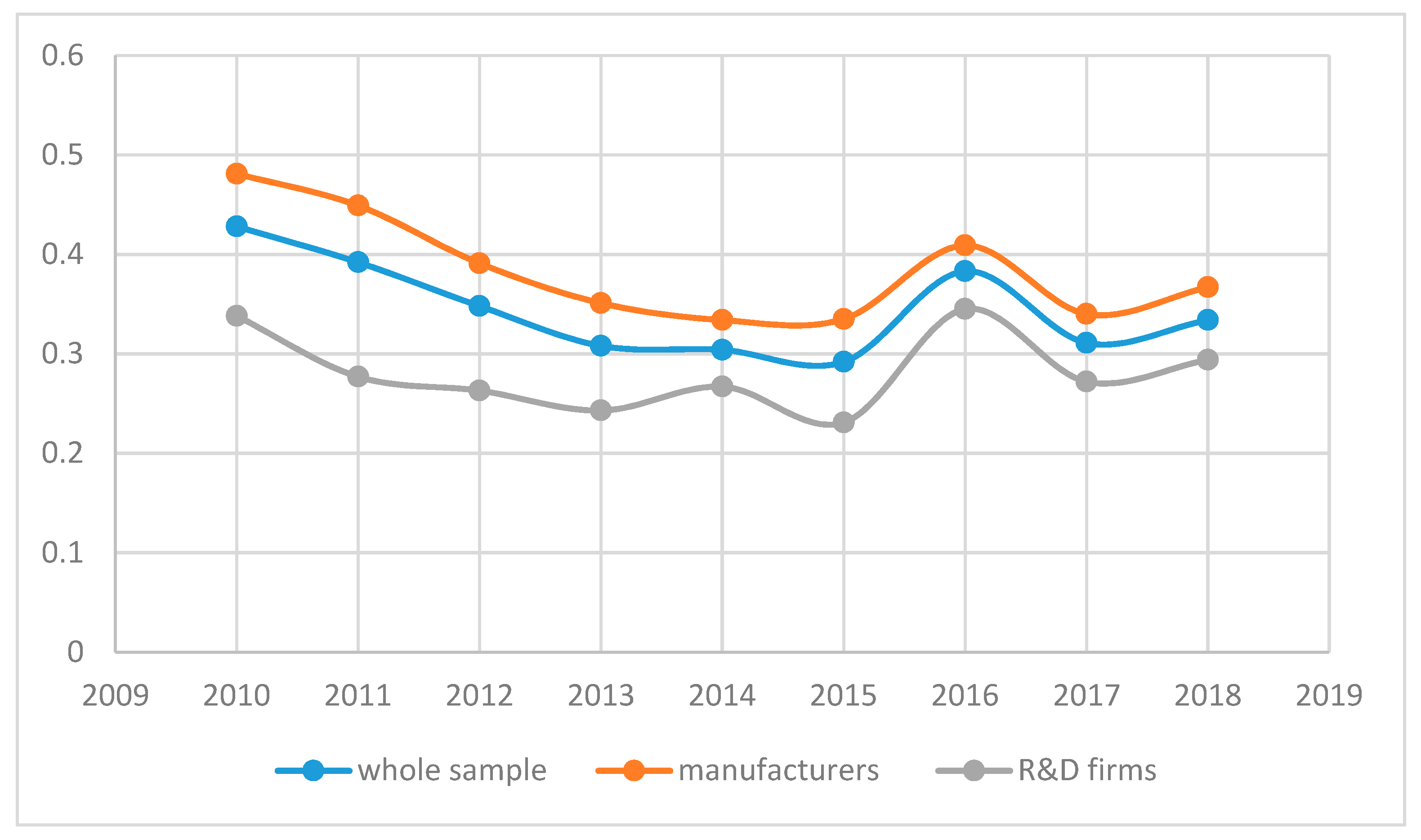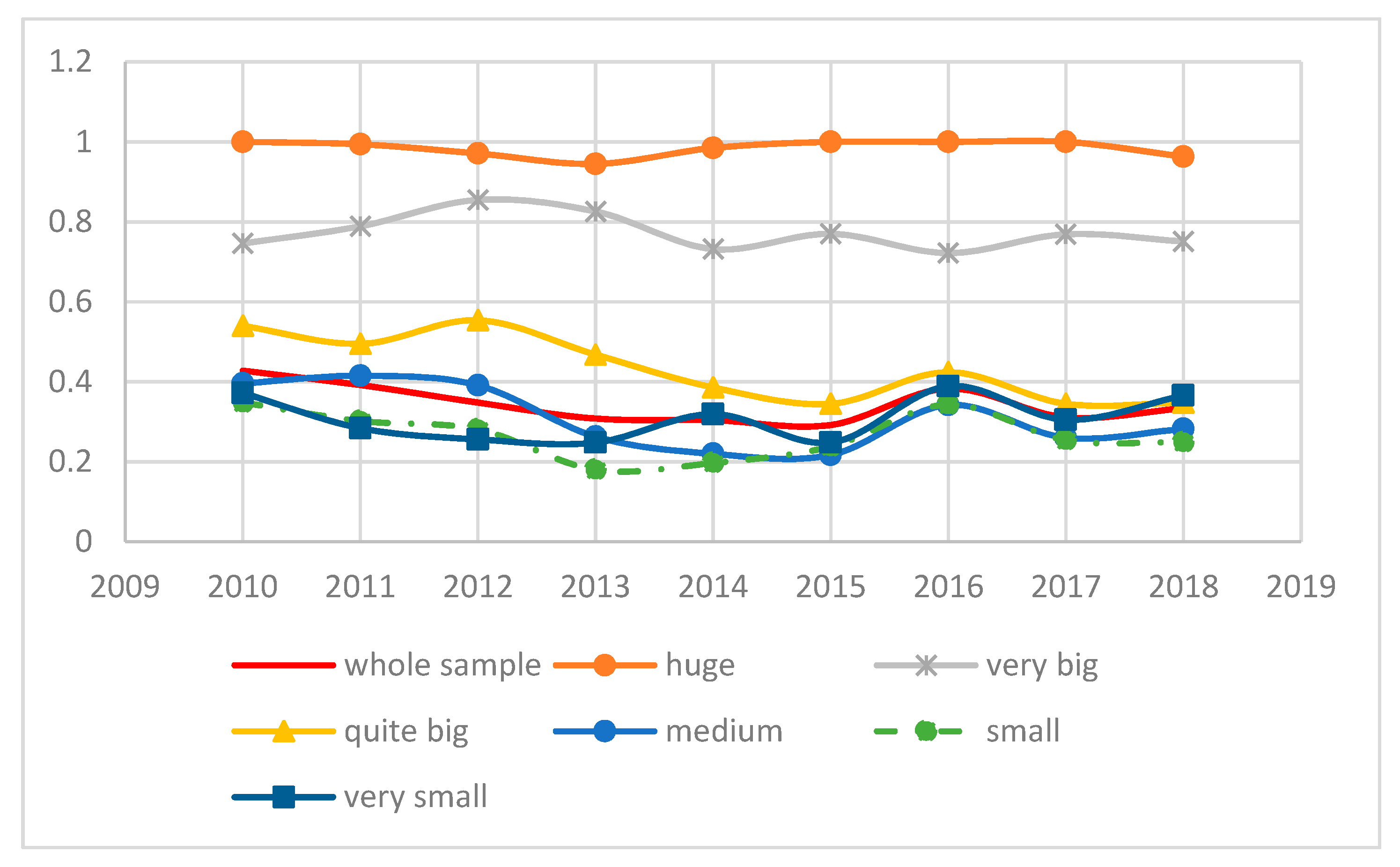LR test of σ²_u = 0 distributed as X²(1). * p < 0.1; ** p < 0.05; *** p < 0.01.

and

Table 5. Variables correlated with efficiency, random effects estimations. Dependent variable is efficiency.

	Model 5	Model 6	Model 7	Model 8
profit_margin	0.1531 ***
	(5.33)
Germany	0.0702	0.1064 *	0.0740	0.0908 *
	(1.23)	(1.85)	(1.41)	(1.70)
Spain	−0.0210	−0.0598 **	0.0304	0.0427
	(0.55)	(2.04)	(0.66)	(0.87)
France	0.0093	0.0504	−0.0150	0.0128
	(0.19)	(1.08)	(0.32)	(0.28)
Sweden	0.2779 ***	0.2420 ***	0.2280 ***	0.2922 ***
	(3.07)	(3.23)	(3.32)	(3.78)
Italy	0.1375 **	0.1488 ***	0.1529 ***	0.1336 ***
	(2.52)	(2.74)	(2.86)	(2.78)
UK	0.1340 ***	0.1538 ***	0.1041 **	0.1295 ***
	(3.44)	(3.91)	(2.51)	(3.70)
Manufacturers	0.0619 *		0.1534 ***
	(1.93)		(4.81)
Huge	0.1189 ***			0.1649 ***
	(2.63)			(3.72)
Verybig	0.1277 ***			0.1247 ***
	(4.28)			(4.06)
Quitebig	0.0233 *			0.0218
	(1.71)			(1.56)
year2014	−0.0778 ***	−0.0736 ***	−0.0625 ***	−0.0728 ***
	(8.64)	(7.67)	(7.14)	(7.90)
year2015	−0.1712 ***	−0.0792 ***	−0.0558 ***	−0.1596 ***
	(6.11)	(6.84)	(7.03)	(5.51)
year2016	0.0366 ***	0.0450 ***	0.0430 ***	0.0430 ***
	(4.09)	(4.52)	(4.78)	(4.46)
cash_flow		0.1661 ***
		(5.83)
Biotech		−0.1298 ***		−0.0421
		(4.42)		(1.44)
Medium		−0.0349 **
		(2.48)
Small		−0.0648 ***
		(3.62)
Verysmall		−0.0092
		(0.33)
collection_period			−0.0226 ***
			(3.97)
employee_cost				−0.3701 ***
				(7.83)
_cons	0.2786 ***	0.3767 ***	0.2257 ***	0.4312 ***
	(7.92)	(15.55)	(6.51)	(19.16)
LR test of σ2u = 0: X2(1)	1306.01 ***	1656.88 ***	2561.80 ***	1156.37 ***
LR test of σ2u = 0: p value	0	0	0	0
Number of observations	1547	1344	1850	1353

Notes: The table summarizes the results from a pure Random-effects estimation of Equation (5). Dependent variable is efficiency computed in Stage 1. Cons stands for the intercept. For the rest of variables, see main text. Data are organized in a panel varying across firms and time over 2010–2018. Robust standard errors clustered at the firm level. LR test of σ²_u = 0 distributed as X²(1). * p < 0.1; ** p < 0.05; *** p < 0.01.

and Figure 3 and Figure 4 summarize some summary statistics about the efficiency of the firms that encompass our sample, as obtained employing DEA in our sample on a yearly basis.

The mean efficiency for the entire sample and over the period 2010–2018 is 0.341. Thus, firms in our sample could increase their efficiency on average in 0.659 points or 65.9%. It seems a reasonable figure. Reference [6] report values of efficiency between 0.42 and 0.58. Their sample is made up by US firms; it seems sensible to think that US firms are, by and large, more efficient than their European counterparts because the general level of efficiency of the US economy is larger and its regulatory burden is smaller. Furthermore, US pharmaceutical firms are larger, on average, than European firms and, as we shall argue below, our results suggest that larger firms are more efficient. The standard deviation is 0.265, which suggests a noticeable degree of dispersion in the sample.

The results are not very different from those obtained by [33]; they find that the average efficiency for a sample of Japanese firms is 0.68 for 1983–1987 and 0.47 for 1988–1993.

If we classify the firms according to their main activity, we find that the mean efficiency for the manufacturers is 0.381 whereas for the R&D firms the figure is smaller, 0.281. This is a somewhat surprising result: the common practice in the industry whereby manufacturers outsource some activities to R&D and biotechnological specialized companies like CROs would suggest on a priori grounds that the former be more efficient that the latter. Otherwise, the outsourcing could be questioned on economic grounds. This is not what we find, however.

One possible explanation for our results is that many manufacturers have been in the market longer, and their historical performance have endowed them with expertise, knowhow and managerial practices which have increased their productivity. This is related to the phenomenon called learning curve in engineering or learning by doing in economics. A classical example is provided by [49], who noticed that the number of hours necessary to produce an airframe was a decreasing function of the number of airframes already produced. Instead, many R&D firms are still relatively young; it is feasible, therefore, that there is still room for them to optimize their processes and value chains and improve their productivity and efficiency.

In addition, the R&D activity in order to develop new drugs is very risky. Success rates are low. Only a modest percentage of molecules are able to complete clinical phases successfully and enter the final market. Reference [50] report that only 10.4% of the drugs entering the clinical stage gain approval by the US Food and Drug Administration (FDA). Biotechnological firms displaying small sizes and relatively reduced pipelines may thus be very affected by failures in the R&D stage. These episodes, in turn, will entail lower levels of productivity.

Notice also that the standard deviation for R&D firms is comparatively high, 0.251. In fact the coefficient of variation, as measured by the ratio standard deviation to mean, is higher for this category. This implies that heterogeneity is more pronounced for this kind of firm.

In order to assess the connection between relative efficiency and size, we have created six categories of firms. Five of these categories (from very big to very small) are linked to the intervals delimited by the 95, 75, 50 and 25 percentiles of real turnover over the period. In particular, the classification is as follows:

• Huge: if the average real turnover over the period exceeds 2000 million euros.
• Very big: if the average real turnover is less or equal than 2000 million euros and higher than 426.92 million euros.
• Quite big: if the average real turnover is less or equal than 426.92 million euros and higher than 38.86 million euros.
• Medium: if the average real turnover is less or equal than 38.86 million euros and higher than 8.10 million euros.
• Small: if the average real turnover is less or equal than 8.10 million euros and higher than 2.10 million euros.
• Very small: if the average real turnover is less or equal than 2.10 million euros.

Table 2 displays summary statistics for relative efficiency classified according to these categories. The largest companies in the sample, those with turnover larger than 2000 million euros, have the highest level of efficiency in the sample, 0.98. In other words, most of them encompass the efficient frontier or are very close to it. There is very little dispersion within this category and the coefficient of variation is almost negligible.

For very big companies, with turnover roughly between 500 and 2000 million euros, efficiency is also remarkably high, 0.765 in average terms. The potential gains in efficiency for this category are only around 25% on average. Firms in the next turnover interval have a smaller record, 0.425. Medium-size firms register lower levels of efficiency on average, 0.312; this is slightly below the figure for the whole sample and period, 0.341.

Small firms, with turnover between 2.10 and 8.10 million euros, register the smallest value of average efficiency, only 0.267. Interestingly, their record is worse than that of the very small firms, with turnover below 2.10 million euros: this last category attains an indicator of 0.318, slightly above medium size firms. This result is consistent with [35], which find that small pharmaceutical firms display smaller levels of efficiency for the case of India.

Higher degrees of flexibility and capacity to adapt to the environment, more agile management and lower levels of conflicts among partners which characterize very small firms may be behind this result. The comparatives advantages provided by specialization may also play a role.

The performance within those categories, as reported by the coefficient of variation, is not uniform. Dispersion is maximum for the very small firms (0.9), whereas more limited for very big firms (0.267). Dispersion in the other categories is similar and quite high: between 0.6 and 0.71.

The implications of these results are interesting. There is not a monotonic, clear cut relationship between size, as captured by turnover, and relative efficiency. Our findings suggest that larger firms are more efficient but only beyond a certain threshold of income, located around 500 million euros. Companies above this figure are considerably more efficient, suggesting the possibility of scale economies for high levels of turnover. Firms with turnover between 38 and 500 thousand million euros also perform better than the whole sample, although their particular advantage amounts just to less than 10 points.

Intermediate and small firms do not profit from scale economies neither from the flexibility and specialization associated to very small firms, and therefore register the poorest results as far as efficiency is concerned.

Table 3 and Figure 3 provide the dynamic context to these results by detailing the performance over the years 2010–2018. Average efficiency plummets from the beginning of the period until 2015, to recover thereafter. In year 2017, efficiency falls again, to increase in 2018, but it does not recover to the levels attained before 2010. Between 2010 and 2018 efficiency diminishes by almost 10 points. The decrease is especially acute for manufacturers, whereas R&D firms only lose 4 points on average.

These results are consistent with [6], who also document a decrease in efficiency for most of the firms in their sample for 2010–2015.

Figure 4 portrays the behavior of firms over time classified according to their size. The largest companies exhibit a fairly consistent performance over time. Instead, for quite big companies the fall of efficiency between the beginning and end of the period is almost 20 points.

At the beginning of the period, in 2010, the efficiency of quite large firms was well above that of the entire sample, while this is not the case anymore in 2018. This category has been affected the most by the drop of efficiency over time.

Medium-sized and small firms exhibit a reduction of 10 points over time, whereas very small firms register a rather stable performance.

5. Stage 2: Variables Correlated with Efficiency

5.1. Overview

In the second stage of this research we have performed a regression analysis in order to explore several aspects of the firms’ economic setting and management which may be correlated with efficiency. Efficiency is proxied by the efficiency scores obtained in the first stage, as detailed in Section 4.

The basic framework is a statistical model described in very general terms by Equation (5):

$$\theta =f\left(x;\upsilon \right)$$

(5)

where θ is a vector containing the efficiency scores, x is a matrix of covariates and υ is the error term.

There are several statistical issues to be considered here.

First, the literature has not reached a consensus about the data generation process underlying Equation (5). Researchers have widely used the Tobit model and ordinary least squares (OLS) (see, for example, [35,51]).

Since the efficiency scores are censored at a maximum of 1 by construction, the Tobit specification seems especially appropriate for this analysis. In addition, References [52,53] argue that OLS provide consistent estimates which are quite similar to those obtained with Tobit and are, therefore, a convenient procedure. Reference [54] show, by means of Monte Carlo simulations, that OLS and Tobit outperform other procedures when employed in the second stage of DEA analyses.

Reference [36], however, have argued that the true data generation process for the efficiency scores is not a censored but a truncated distribution; they discard the analysis of the efficiency scores performed according to Tobit or ordinary least squares because this assessment would not rely on the true distribution of the data. With censored data, the true value of the variable is not known because of the measurement scale; in this particular case, since efficiency has an upper bound of 1. With truncated data, instead, the true value of the variable is unknown because of the sample limitations. The difference in practice between a censored and a truncation distribution may be unclear.

Furthermore, they claim that the efficiency scores are affected by serial correlation. Since the Tobit procedure does not correct for this problem, the estimates obtained from the Tobit model are, in their view, biased. This issue is also controversial, since [54] have argued that OLS and Tobit procedures are valid even if the X variables are correlated.

Reference [36] propose an alternative estimation technique which employs a truncated model, computes new standard errors by bootstrapping the data and corrects the biases in the estimates. There are downsides for this procedure. Reference [53] argues that the Simar–Wilson estimates lack robustness. Furthermore, the Simar–Wilson technique is convoluted and intensive in computing time. Furthermore, as we shall show below, the point estimates computed by the Simar–Wilson method are bigger than those obtained by Tobit or ordinary least squares, although the difference may not be very relevant in applied research.

The debate is still open. According to [53], the controversy about the correct statistical model underlying the data is ultimately methodological and exceeds the scope of our research. By and large, we agree with [53] and think that Tobit and ordinary least squares have helped obtain valid insights about the efficiency in numerous industries or activities, and thus can be employed in applied research.

Meanwhile, since the controversy has not been settled yet, we have decided to adopt a conservative strategy, employ the three methods and compare their results.

Second, the data we are going to use to estimate Equation (5) encompass a panel and hence comprises observations from firms at different points in time.

As is well known, panel data can be assessed by fixed effects or random effects models. [55] shows that Tobit models with fixed effects produce coefficients which are overestimated and asymptotic variances which are biased downwards. Moreover, our specification includes as regressors time-invariant characteristics of firms (such as country of origin, for example); these characteristics would be perfectly collinear with the terms capturing the idiosyncratic features of firms in a fixed effects model. In this case we cannot employ a Hausman test to compare the fixed effects and random effects models because our model cannot be specified within a fixed effects setting.

These considerations advise the utilization of random-effects models. This is the approach followed, for example, by [35].

Finally, at this point we are searching for correlations among efficiency and different aspects of firm idiosyncrasies and management. Looking for causality relationships exceeds the scope of this paper and is left for future research.

We shall start by discussing the main qualitative implications of this exercise, for reasons which will be apparent below.

5.2. Qualitative Implications

5.2.1. Tobit Estimation

Typically, a Tobit model distinguishes between the latent or unobservable dependent variable and the observable dependent variable, where the observed variable is a censored version of the unobserved.

Equation (6) represents a random-effects Tobit specification for the second stage of our analysis:

$${\theta }_{it}^{*}= x_{it}\beta +u_i+{\epsilon }_{it}$$

(6)

$${\theta }_{it }=1 if {\theta }_{it}^{*}\ge 1$$

$${\theta }_{it }= {\theta }_{it}^{*} if 0\le {\theta }_{it}^{*}\le 1$$

$${\theta }_{it }=0 if {\theta }_{it}^{*}\le 0$$

$$i=1, 2, \dots , n.$$

$$t=2010, 2011, \dots , 2018$$

wre θ_it* is the latent or unobservable efficiency, θ_it is the observable efficiency, x_it is a matrix of covariates, β is a vector of coefficients, u_i is the time invariant component of the error term, ε_it is the time-varying component of the error term, i indexes firms and t time.

In the estimation of Equation (6) we have included several indicators as covariates in order to capture different dimensions of firms, such as main activity, size, margins, financial management and personnel costs. We have also included time dummies to capture the impact of the business cycle and country dummies to allow for idiosyncratic aspects related to the markets where firms operate. The data are structured in a panel over the period 2010–2018 in order to exploit both the cross section and time variations.

Table 4 shows a first set of results obtained from the estimation by maximum likelihood of the model described by Equation (6). In order to avoid multicollinearity among the regressors, we have not included all covariates simultaneously; instead, we have added them sequentially, conforming different specifications of the baseline Equation (6). In other words, Equation (6) describes Models 1–4, the differences among them being the variables considered in x_it in each case.

To correct for heteroskedasticity, estimations have been performed with the observed information matrix (OIM) corrected standard errors. In this particular case, the variance-covariance matrix of the estimators is the matrix of second derivatives of the likelihood function. This correction for heteroskedasticity is robust to the violation of normality if distribution is symmetrical.

The last lines of Table 4 include the results from a Lagrange multiplier Breusch–Pagan likelihood ratio test of whether the variance of the time invariant component of the error term is equal to zero. This test is can be regarded as an indirect text of the appropriateness of the random effect model. The null hypothesis of equality to 0 of the variance of the u_i component of the error term is rejected at the 99% significance level for the four models, hence supporting the utilization of the random-effects model.

Dummies for countries capture different aspects: on the one hand, cultural and institutional aspects and managerial practices ([38]). On the other, regulatory and microeconomic and macroeconomics conditions of the particular markets where the firms operate. Regulatory aspects and institutional and macroeconomic conditions in the host country have been shown to impact the performance of multinational firms ([56,57]).

Dummies for the United Kingdom (UK), Italy and Sweden are positive and highly significant in all specifications, implying that the institutional framework in these countries, the size of their markets and/or their macroeconomic and institutional conditions affect the efficiency of firms positively. The dummy for Germany is also positive and significant in two specifications (models 2 and 4), although in one of them at a smaller significance level (90% in model 4).

Instead, the dummies for Spain and France display positive and negative signs and are not significant.

UK pharmaceutical firms feature a swift decision-making process which facilitates a successful and fast adjustment to changing market conditions ([58]). Moreover, the level of distortions in the UK economy is low and factor markets are relatively flexible. In addition, the dynamic biotechnological landscape of the country has allowed the surge of alliances and collaborations. These facts may explain the positive sign of the UK dummy.

German firms typically work in less-flexible environments than their British counterparts; their access to bank funding, though, is comparatively easy. Since sound finance is one important determinant of firms’ success, as will be detailed below, the availability of funding seems quite relevant for the performance of companies in the sector and help explain the positive sign of the dummy.

The Italian industry is populated by highly skilled, agile firms, with a large component of exports and close ties to US companies. These companies encompass an important hub for foreign investment in the industry, which in turn enhances the productivity of local firms through technology diffusion and learning by watching.

Swedish pharmaceutical and biotechnological firms benefit from a market with limited regulation where bureaucracy is kept at a minimum, government support and a highly skilled workforce. These aspects would explain the successful performance of the Swedish pharmaceutical industry.

The positive signs of the country dummies, therefore, are in accordance with particular features of their institutional frameworks and/or industries.

These features, however, are not present in the French and Spanish cases. The French pharmaceutical market has historically been very protected by an outdated industrial policy. Spanish companies have been damaged by a rigid labor market and a low level of interaction between universities, research centers and firms.

We have also captured the main activity of the firms by means of dummies variables. The dummy manufacturers is equal to 1 for those firms whose main activity corresponds to NACE codes 2110 and 2120, and 0 otherwise. Conversely, the dummy biotech is 1 for firms included under the 7211 NACE code and 0 otherwise.

The dummy manufacturers are positively and significantly correlated with efficiency (columns 1 and 3), while biotech displays a negative and significant correlation in one model (column 2) and is not significant in the other (column 4). Overall, these findings are in accordance with those reported in Section 4 above, which suggest consistently higher levels of efficiency for firms engaged in the production and commercialization of pharmaceutical articles.

Dummies for size have been assigned according to the thresholds detailed in Section 4 above. Again, the results for the estimations agree with the trends reported in the previous Section. Firms characterized by large sizes, as conveyed by their levels of turnover, are more efficient than their counterparts, since the dummies huge and very big are positively and significantly correlated with efficiency (Models 1 and 4). The dummy that is quite big is positive but not significant.

The positive correlation between size and efficiency, however, holds only for the first two categories we defined, i.e., for sales larger than 426.92 million euros or the 95 percentile in the distribution. For companies with real turnover between 38.86 and 426.92 million euros results are inconclusive.

Those companies whose level of sales is less or equal than 38.86 million and more than 2.10 million euros register smaller efficiency figures ceteris paribus, since the dummies medium and small are negative and significant (column 2). Finally, we do not find a significant correlation between the dummy capturing the very small level of sales and efficiency (column 2). This is not surprising since firms with sales lower than the 25% percentile register poor levels of efficiency in some years but are capable of surpassing the figure attained by medium and small others.

The results for the dummy variables reflecting size and activity are thus consistent with those reported in the previous section. They are also in accord with [35], who disclose a negative correlation between size and efficiency for a sample of Indian pharmaceutical firms.

Let us turn to the discussion of the variables capturing other aspects of firms in the industry.

As portrayed by column 1 of Table 4, the profit margin is positively and significantly correlated, at the 99% significance level, with efficiency. This means that more efficient firms operate with higher margins. This result makes sense because the industry we are scrutinizing provides goods and services characterized by high added value which can be reflected in large margins. In fact, Reference [59] argues that deviations from trend in profit margins are highly correlated with expenditure in R&D for pharmaceutical companies, thus confirming the links between efficiency, margins and R&D.

Interestingly, this finding suggests that successful firm strategies in this sector are featured by both high margins and high intensity of resource utilizations, at the same time. It is common to see that companies tend to choose to focus either on the achievement of high profits per unit or in the optimization of the installed capacity. This dichotomy, however, is not present in the companies in the pharmaceutical industry, according to our results.

The literature has documented that cash flow influences R&D expenditure in the case of the industry we are considering ([60]). Reference [61] provide some additional evidence since they find that, for the Spanish firms, the proportion of expenditure in R&D financed with internal resources is 75% for pharmaceuticals and 40% for the rest of the industries. Again, we are confronted with another differential feature of this industry. Whereas it is commonly accepted that firms should heavily rely on external funding and increase their profitability through financial leverage, the empirical evidence for this industry suggests that successful companies enjoy comparatively low ratios of indebtedness. This prudent financial structure is consistent with the high risk and long maturing period associated with the R&D activity.

To test this idea in our sample, we have included in the analysis some variables which capture particular elements of financial management. Column 2 shows that cashflow (as a percentage of sales) is indeed positively and significantly correlated with efficiency. The level of significance is very high, 99%.

Column 3, in turn, displays the estimation results when the variable collection period is included as a regressor in the baseline specification. The point estimate is negative and significant at the 99% level. Higher collection periods increase the amount of working capital necessary to run the daily activity of the firm, while shorter spans imply a sounder financial management. Our findings, therefore, are consistent with the literature, and stress the importance of exhibiting solid, well-financed balance sheets in order to register high levels of productivity. In more detail, Reference [35] argue that the low efficiency scores achieved by some firms in their sample is associated to their inability to access financial resources.

Column 4 includes a variable capturing the cost of labor, average cost per employee, as a percentage of sales. It is highly significant and negatively correlated with efficiency.

In terms of the validations of Models 1–4, and as stated above, the literature has shown that the Tobit model provides consistent estimates ([52,53,54,62]).

Moreover, it has been argued that the severity of the problem implied by the presence of heteroskedasticity in Tobit models is a function of the degree of censoring. In our case, censoring is limited, and affects only to 6–7% of the data.

Since the estimations have been performed with OIM corrected standard errors, they are robust to the presence of heteroskedasticity. These standard errors are also robust to the violation of normality if the distribution is symmetric.

Finally, and as detailed below, results from Tobit are quite similar to those obtained by random-effects models. All these considerations lend countenance to the models described in this subsection.

5.2.2. Classical Estimation

In order to assess the robustness of these findings we have performed two complementary analyses.

First, we have considered a pure random-effects model, as described by Equation (7).

$${\theta }_{it}=x_{it}\beta +u_i+{\epsilon }_{it}$$

(7)

where θ_it is efficiency, x_it is a matrix of covariates, β is a vector of coefficients, u_i is the time invariant component of the error term, ε_it is the time-varying component of the error term, i indexes firms and t time.

The estimation has been carried out with robust standard errors, in the spirit of [63,64,65], clustered at the firm level. This procedure is widely recommended in the literature in these types of estimations ([66]).

Table 5 summarizes the specification and results for Models 5–8, estimated according to (7). We see that the main conclusions obtained from the Tobit specification regarding the correlation of efficiency with selected variables carry over to the classical, pure random effects specification. The only remarkable differences are related to the dummy for Spain, which is now negative and significant at the 95% level (Model 6), and the dummy quite big, now significant at the 90% level.

Furthermore, the point estimates of the coefficients are very similar in the censored and the non-censored model. These results are reassuring and consistent with [52,53], who document this kind of similarity when Tobit and ordinary least squares are employed in the second stage analysis.

The last two lines of Table 5 display the results from the Lagrange multiplier Breusch–Pagan test for the presence of random effects. The null hypothesis of no random effects is rejected at conventional levels.

In terms of the validation of Models 5–8, we can invoke the result according to which OLS produces unbiased and consistent estimates because of the central limit theorem for large enough samples. In addition, the literature has also shown the consistency of OLS second-stage estimators for the particular case of DEA analyses. Moreover, cluster robust standard errors yield estimates that are robust to the presence of heteroskedasticity and correlation in the error term.

5.2.3. Simar–Wilson Estimation

We have employed the [36] methodology as a further robustness test. Accordingly, we have replicated the estimations described above, this time employing their technique. These are Models 9–12, whose detailed specifications and results are displayed in

Table 6. Variables correlated with efficiency, Simar–Wilson estimations. Dependent variable is efficiency.

	Model 9	Model 10	Model 11	Model 12
profit_margin	0.3089 ***
	(9.31)
Germany	0.1287 ***	0.1562 ***	0.1405 ***	0.1204 ***
	(4.43)	(4.93)	(3.64)	(4.09)
Spain	−0.0356	−0.0971 ***	−0.0098	0.0053
	(1.36)	(3.25)	(0.24)	(0.20)
France	0.0342	0.0684 *	−0.1606 ***	−0.0364
	(0.92)	(1.72)	(3.06)	(0.97)
Sweden	0.2958 ***	0.2602 ***	0.3352 ***	0.3539 ***
	(8.04)	(6.04)	(7.06)	(8.41)
Italy	0.1548 ***	0.1539 ***	0.2307 ***	0.1506 ***
	(6.13)	(5.67)	(6.41)	(5.99)
UK	0.1439 ***	0.1596 ***	0.1370 ***	0.1396 ***
	(6.89)	(7.33)	(4.97)	(6.81)
Manufacturers	0.0859 ***		0.3157 ***
	(4.54)		(10.51)
Huge	0.7812 **			0.8741 **
	(2.06)			(2.45)
Verybig	0.4284 ***			0.3849 ***
	(9.48)			(8.47)
Quitebig	0.0552 ***			0.0678 ***
	(2.98)			(3.63)
year2014	−0.0994 ***	−0.1072 ***	−0.0982 ***	−0.0977 ***
	(4.20)	(4.16)	(2.80)	(3.77)
year2015	−0.4586 ***	−0.1540 ***	−0.1161 ***	−0.4179 ***
	(9.43)	(5.15)	(3.40)	(8.48)
year2016	0.0652 ***	0.0651 ***	0.0902 ***	0.0785 ***
	(3.04)	(2.76)	(3.07)	(3.66)
cash_flow		0.3351 ***
		(8.31)
Biotech		−0.1790 ***		−0.0229
		(8.07)		(1.15)
Medium		−0.1294 ***
		(6.36)
Small		−0.1091 ***
		(4.63)
Verysmall		0.0192
		(0.60)
collection_period			−0.0568 ***
			(4.11)
employee_cost				−0.6340 ***
				(10.95)
_cons	0.1328 ***	0.3237 ***	−0.0524	0.3822 ***
	(6.01)	(15.50)	(1.24)	(20.23)
Number of observations	1446	1257	1741	1264

Notes: The table summarizes the results from the Simar–Wilson estimation of Equation (5). Dependent variable in the estimations is efficiency. Data are set in a panel varying across firms and time. * p < 0.1; ** p < 0.05; *** p < 0.01.

.

Once again, we see that the basic findings obtained by the Tobit and classical random effects estimations regarding the sign and significance of covariates carry over when the [36] procedure, based upon a truncated distribution for the data and bootstrapping, is employed.

As reported above, this tool aims to remove the alleged bias in the estimation due to correlation among residuals. It computes new standard errors and corrected parameters. In contrast to the Tobit and classical frameworks, the literature has not provided enough evidence yet to illustrate the properties of this estimator.

5.3. Quantitative Implications

From the comparisons of Table 4, Table 5 and Table 6 we observe that Tobit and pure random-effects models yield point estimates which are rather similar. Instead, estimates obtained by the Simar–Wilson methodology are larger.

In contrast to what happens in the classical regression model, the marginal effect or impact of the individual regressor x_j on the dependent variable, defined as:

$$\frac{\partial \theta }{\partial x_j}$$

is not directly measured by the point estimates of regressions estimated by Tobit or Simar–Wilson methodologies, since they are non-linear models.

In order to extract more quantitative implications of the different estimations described in Section 5.2 above, we have computed the marginal effects of selected variables on efficiency implied by these two methods.

Basic results are displayed in

Table 7. Comparison of marginal effects, Tobit, Simar–Wilson and random effects estimations.

Variable	Tobit	Simar–Wilson	Random Effects
Profit margin	0.1511	0.2053	0.1531
Cash flow/income	0.1628	0.2189	0.1661
Collection period	−0.0223	−0.026	−0.0226
Employee cost	−0.3683	−0.4215	−0.3701

Notes: The table details the marginal effects on efficiency levels of each one of the variables displayed in the first column. These marginal effects have been recovered from the Tobit (Models 1–4) and the Simar–Wilson (Models 9–12) estimations. The last column displays the marginal effects obtained in the pure random-effects models (Models 5–8) to facilitate the comparison; since this framework is linear, the marginal effects coincide with the point estimates of the variables as reported in Table 5.

. In order to facilitate comparisons, we have added the point estimates obtained by the pure random-effects estimation.

The variable exerting the highest impact on efficiency is employee cost. According to our results, an increase of one unit in the employee cost reduces efficiency in an amount which is comprised in the interval (0.368, 0.42).

If the profit margin rises in one unit, the correspondent increase in efficiency is around 0.15–0.2. The improvement of the financial position (as captured by cash flow/income) in one unit brings about a positive change in efficiency of 0.162–0.218. Finally, the increase of the collection period in one unit reduces efficiency around 0.02.

In our view, these findings have some interesting economic implications and may be useful for managers, owners and other stakeholders of firms in the industry. The efforts to contain personnel costs and increase margins translate directly into higher levels of productivity. Firms in the industry should also strive to achieve an adequate combination of external and internal finance, aligned with the risky and slow-paced nature of R&D activities.

There are implications for policymakers and policy analysts as well. Efficiency in the pharmaceutical sector, according to the empirical evidence presented here, hinges on the sound functioning of labor markets and financial markets. Measures to improve their behavior may have a noticeable impact on the performance of the firms in the industry.

It is apparent from Table 7 that the marginal effects obtained by the Tobit and the classical specifications are remarkably close, whereas those yielded by the Simar–Wilson procedure are slightly larger. It is important to notice that the difference among the Tobit/pure random effects results, on the one hand, and the Simar–Wilson, on the other, is smaller regarding the marginal effects (Table 7) that if we compare the point estimates (Table 4, Table 5 and Table 6).

This fact has several interesting implications:

-

As far the particular goal of this subsection is concerned, the Simar–Wilson tool implies marginal effects slightly larger (about 15–35%) but of the same order of magnitude than those obtained from Tobit/pure random-effects model.

-

In general terms, more research at the theoretical level and probably Monte Carlo simulations are necessary to know in more detail the properties of the Simar–Wilson estimator. This exceeds the scope of this paper.

-

The Simar–Wilson procedure may be useful for applied research, especially in conjunction with other methodologies, although it has a higher cost in computing time if compared with Tobit or classical models.

6. Concluding Remarks

The pharmaceutical industry has experienced deep changes in the last few decades. The cost of R&D has soared while market conditions have become tougher. Companies have confronted these challenges by different strategies such as mergers, acquisitions, outsourcing and alliances. It remains an open question whether these transformations have brought about an increase in the efficiency of the firms that make up the industry.

We examine this issue employing disaggregated microdata from a large sample of European medium and large firms belonging to the pharmaceutical and biotechnological industry. In the first stage of our research, we perform a non-parametric DEA analysis of efficiency over the period 2010–2018. In the second stage we analyze which potential features of the environmental framework and management are correlated with efficiency by regression techniques.

The consideration of a large sample of European firms, disaggregating by main activity and isolating the performance of biotechnological firms is a novel feature of this paper. The comparison of the results provided by the Tobit, classical and Simar–Wilson frameworks for the second stage is also a contribution of the investigation presented here.

The main insights from our analysis are the following:

-

The average level of efficiency in the industry is moderate, 0.341. This figure is not far from results obtained by other studies for alternative samples. Efficiency exhibits a decreasing trend over the years 2010–2018.

-

Efficiency levels display a large level of heterogeneity when particular dimensions of companies are considered. Efficiency is higher for those companies whose main activity is manufacturing of pharmaceutical products than for firms focused on R&D activities. This result may be traced to the relative youth of R&D firms, which cannot fully exploit the learning curve yet. The specialization of this kind of firms in a few projects, characterized by low rates of success, may also be a relevant factor in this respect.

-

We find a complex relationship between size and efficiency. By and large, bigger firms are more efficient, but only beyond the threshold of 426.92 million euros of turnover per year. Medium-size and small firms register the poorest levels of efficiency, whereas very small firms perform slightly better. This suggests that firms may benefit from either scale economies or high levels of specialization, while the middle ground does not yield good results.

-

Our findings suggest that sound financial structures, lower employee costs and higher margins are correlated with higher levels of efficiency. Moreover, the idiosyncratic aspects of the country of origin of the firms may foster or jeopardize productivity.

Our results convey some messages for policymakers. The survival and buoyancy of companies in the pharmaceutical industry seems closely linked to the sound functioning of the labor and capital markets. The experience of selected countries, in particular the UK, suggests as well that the existence of agile, dynamic biotechnological firms is beneficial for the whole sector.

Finally, the higher levels of efficiency obtained for larger firms suggest that mergers and acquisitions may enhance the performance of pharmaceutical companies due to the influence of scale economies. These financial transactions should not be discouraged or jeopardized by policymakers on the basis of an allegedly anti-competitive strategy. It is important to keep in mind that the pharmaceutical and biotechnological industry relies heavily on R&D, and that R&D is only feasible for firms if their size is big enough.

We have also found that very small firms display a sounder behavior than medium size companies. The link between size and performance for the sector is thus nuanced. This suggests that industrial policies intending to enhance the sector should be horizontal rather than vertical: instead of featuring active interventions in favor of a particular firm size, it is better to adopt a less activist stance since it is hard to determine on an a priori basis which is the efficient scale of operations.

Our investigation has several limits. The time horizon is relatively short; it would be convenient to increase it whenever new data are available. We have computed efficiency scores in Stage 1 only by a non-parametric technique, DEA; another computation by means of parametric SFA would be useful to check whether efficiency scores are very sensible to the tool employed.

In stage 2 we have investigated the correlations among efficiency scores and other variables, but we have not explored the direction of causality among them. This last issue could be addressed by introducing lags and leads of the variables and/or employing other econometric techniques, such as general methods of moment or instrumental variables.

One of the techniques we have employed in Stage 2 is the Simar–Wilson estimation. It seems to be useful in applied work, especially in combination with other techniques. More evidence about its performance would be convenient, nonetheless.

Finally, and although country dummies have provided useful information about the potential impact of institutional and economic aspects on efficiency, they are ultimately dummies or the measure of our ignorance; it would be interesting to go one step further and characterize the specific features of the various countries which enhance or jeopardize efficiency. This could be done by introducing macroeconomic and institutional variables in the Stage 2 models.

These limitations suggest promising directions for new research.

References

1. Lucas, R.E. On the mechanics of economic growth. J. Monet. Econ. 1988, 22, 3–42. [Google Scholar] [CrossRef]
2. Romer, P.M. Increasing Returns and Long-Run Growth. J. Political Econ. 1986, 94, 1002–1037. [Google Scholar] [CrossRef] [Green Version]
3. Romer, P.M. Endogenous Technological Change. J. Political Econ. 1990, 98, S71–S102. [Google Scholar] [CrossRef] [Green Version]
4. Pammolli, F.; Magazzini, L.; Riccaboni, M. The productivity crisis in pharmaceutical R&D. Nat. Rev. Drug Discov. 2011, 10, 428–438. [Google Scholar] [CrossRef] [PubMed]
5. Shimura, H.; Masuda, S.; Kimura, H. A lesson from Japan: Research and development efficiency is a key element of pharmaceutical industry consolidation process. Drug Discov. Ther. 2014, 8, 57–63. [Google Scholar] [CrossRef] [PubMed] [Green Version]
6. Shin, K.; Lee, D.; Shin, K.; Kim, E. Measuring the Efficiency of U.S. Pharmaceutical Companies Based on Open Innovation Types. J. Open Innov. Technol. Mark. Complex. 2018, 4, 34. [Google Scholar] [CrossRef] [Green Version]
7. Rafols, I.; Hoekman, J.; Siepel, J.; Nightingale, P.; Hopkins, M.M.; O’Hare, A.; Perianes-Rodriguez, A. Big Pharma, Little Science? A Bibliometric Perspective on Big Pharma’s R&D Decline. SSRN Electron. J. 2012, 81, 22–38. [Google Scholar] [CrossRef] [Green Version]
8. Gascón, F.; Lozano, J.; Ponte, B.; De La Fuente, D. Measuring the efficiency of large pharmaceutical companies: An industry analysis. Eur. J. Health Econ. 2016, 18, 587–608. [Google Scholar] [CrossRef]
9. Jiang, H.; He, Y. Applying Data Envelopment Analysis in Measuring the Efficiency of Chinese Listed Banks in the Context of Macroprudential Framework. Mathematics 2018, 6, 184. [Google Scholar] [CrossRef] [Green Version]
10. Kumbhakar, S.C.; Lien, G.; Hardaker, J.B. Technical efficiency in competing panel data models: A study of Norwegian grain farming. J. Prod. Anal. 2012, 41, 321–337. [Google Scholar] [CrossRef]
11. Wang, C.-N.; Nguyen, M.N.; Le, A.L.; Tibo, H. A DEA Resampling Past-Present-Future Comparative Analysis of the Food and Beverage Industry: The Case Study on Thailand vs. Vietnam. Mathematics 2020, 8, 1140. [Google Scholar] [CrossRef]
12. Chen, C.F.; Soo, K.T. Some university students are more equal than others: Efficiency evidence from England. Econ. Bull. 2010, 30, 2697–2708. [Google Scholar]
13. Lozano, S.; Gutiérrez, E. A slacks-based network DEA efficiency analysis of European airlines. Transp. Plan. Technol. 2014, 37, 623–637. [Google Scholar] [CrossRef]
14. Lin, B.-H.; Lee, H.-S.; Chung, C.-C. The Construction and Implication of Group Scale Efficiency Evaluation Model for Bulk Shipping Corporations. Mathematics 2020, 8, 702. [Google Scholar] [CrossRef]
15. Zhou, Z.; Jin, Q.; Peng, J.; Xiao, H.; Wu, S. Further Study of the DEA-Based Framework for Performance Evaluation of Competing Crude Oil Prices’ Volatility Forecasting Models. Mathematics 2019, 7, 827. [Google Scholar] [CrossRef] [Green Version]
16. Kuosmanen, T.; Saastamoinen, A.; Sipiläinen, T. What is the best practice for benchmark regulation of electricity distribution? Comparison of DEA, SFA and StoNED methods. Energy Policy 2013, 61, 740–750. [Google Scholar] [CrossRef]
17. Cherchye, L.; De Rock, B.; Walheer, B. Multi-output efficiency with good and bad outputs. Eur. J. Oper. Res. 2015, 240, 872–881. [Google Scholar] [CrossRef] [Green Version]
18. Orea, L.; Llorca, M.; Filippini, M. A new approach to measuring the rebound effect associated to energy efficiency improvements: An application to the US residential energy demand. Energy Econ. 2015, 49, 599–609. [Google Scholar] [CrossRef] [Green Version]
19. Alarenan, S.; Gasim, A.A.; Hunt, L.C.; Muhsen, A.R. Measuring underlying energy efficiency in the GCC countries using a newly constructed dataset. Energy Transit. 2019, 3, 31–44. [Google Scholar] [CrossRef] [Green Version]
20. Ahn, H.; Afsharian, M.; Emrouznejad, A.; Banker, R.D. Recent developments on the use of DEA in the public sector. Socio-Econ. Plan. Sci. 2018, 61, 1–3. [Google Scholar] [CrossRef] [Green Version]
21. Sueyoshi, T.; Yuan, Y.; Goto, M. A literature study for DEA applied to energy and environment. Energy Econ. 2017, 62, 104–124. [Google Scholar] [CrossRef]
22. Odeck, J.; Bråthen, S. A meta-analysis of DEA and SFA studies of the technical efficiency of seaports: A comparison of fixed and random-effects regression models. Transp. Res. Part A Policy Pract. 2012, 46, 1574–1585. [Google Scholar] [CrossRef]
23. Fall, F.; Akim, A.-M.; Wassongma, H. DEA and SFA research on the efficiency of microfinance institutions: A meta-analysis. World Dev. 2018, 107, 176–188. [Google Scholar] [CrossRef] [Green Version]
24. Marchetti, D.; Wanke, P.F. Efficiency in rail transport: Evaluation of the main drivers through meta-analysis with resampling. Transp. Res. Part A Policy Pract. 2019, 120, 83–100. [Google Scholar] [CrossRef]
25. Emrouznejad, A.; Yang, G.-L. A survey and analysis of the first 40 years of scholarly literature in DEA: 1978–2016. Socio-Econ. Plan. Sci. 2018, 61, 4–8. [Google Scholar] [CrossRef]
26. Emrouznejad, A.; Thanassoulis, E. A mathematical model for dynamic efficiency using data envelopment analysis. Appl. Math. Comput. 2005, 160, 363–378. [Google Scholar] [CrossRef]
27. Hu, X.-Y.; Li, J.; Li, X.; Cui, J. A Revised Inverse Data Envelopment Analysis Model Based on Radial Models. Mathematics 2020, 8, 803. [Google Scholar] [CrossRef]
28. Wei, G.-W.; Wang, J. A comparative study of robust efficiency analysis and Data Envelopment Analysis with imprecise data. Expert Syst. Appl. 2017, 81, 28–38. [Google Scholar] [CrossRef]
29. Khezrimotlagh, D.; Zhu, J.; Cook, W.D.; Toloo, M. Data envelopment analysis and big data. Eur. J. Oper. Res. 2019, 274, 1047–1054. [Google Scholar] [CrossRef]
30. You, T.; Chen, X.; Holder, M.E. Efficiency and its determinants in pharmaceutical industries: Ownership, R&D and scale economy. Appl. Econ. 2010, 42, 2217–2241. [Google Scholar] [CrossRef]
31. Mao, Y.; Li, J.; Liu, Y. Evaluating business performance of China’s pharmaceutical companies based on data envelopment analysis. Stud. Ethno-Med. 2014, 8, 51–60. [Google Scholar] [CrossRef]
32. Sueyoshi, T.; Goto, M. DEA radial measurement for environmental assessment: A comparative study between Japanese chemical and pharmaceutical firms. Appl. Energy 2014, 115, 502–513. [Google Scholar] [CrossRef]
33. Hashimoto, A.; Haneda, S. Measuring the change in R&D efficiency of the Japanese pharmaceutical industry. Res. Policy 2008, 37, 1829–1836. [Google Scholar] [CrossRef] [Green Version]
34. Al-Refaie, A.; Wu, C.-W.; Sawalheh, M. DEA window analysis for assessing efficiency of blistering process in a pharmaceutical industry. Neural Comput. Appl. 2018, 31, 3703–3717. [Google Scholar] [CrossRef]
35. Mazumdar, M.; Rajeev, M.; Ray, S.C. Output and Input Efficiency of Manufacturing Firms in India: A Case of the Indian Pharmaceutical Sector; Institute for Social and Economic Change: Bangalore, India, 2009. [Google Scholar]
36. Simar, L.; Wilson, P.W. Estimation and inference in two-stage, semi-parametric models of production processes. J. Econ. 2007, 136, 31–64. [Google Scholar] [CrossRef]
37. Bloom, N.; Lemos, R.; Sadun, R.; Scur, D.; Van Reenen, J. International Data on Measuring Management Practices. Am. Econ. Rev. 2016, 106, 152–156. [Google Scholar] [CrossRef] [Green Version]
38. Bénabou, R.; Tirole, J. Mindful Economics: The Production, Consumption, and Value of Beliefs. J. Econ. Perspect. 2016, 30, 141–164. [Google Scholar] [CrossRef] [Green Version]
39. Aigner, D.; Lovell, C.; Schmidt, P. Formulation and estimation of stochastic frontier production function models. J. Econ. 1977, 6, 21–37. [Google Scholar] [CrossRef]
40. Meeusen, W.; Broeck, J.V.D. Efficiency Estimation from Cobb-Douglas Production Functions with Composed Error. Int. Econ. Rev. 1977, 18, 435. [Google Scholar] [CrossRef]
41. Kumbhakar, S.C.; Parmeter, C.F.; Zelenyuk, V. Stochastic frontier analysis: Foundations and advances. In Handbook of Production Economics; Springer: New York, NY, USA, 2017. [Google Scholar]
42. Charnes, A.; Cooper, W.; Rhodes, E. Measuring the efficiency of decision making units. Eur. J. Oper. Res. 1978, 2, 429–444. [Google Scholar] [CrossRef]
43. Banker, R.D.; Charnes, A.; Cooper, W.W. Some Models for Estimating Technical and Scale Inefficiencies in Data Envelopment Analysis. Manag. Sci. 1984, 30, 1078–1092. [Google Scholar] [CrossRef] [Green Version]
44. Van Dijk, B. Amadeus Database; Bureau van Dijk Electronic Publishing: Brussels, Belgium, 2020. [Google Scholar]
45. Eurostat. Available online: https://appsso.eurostat.ec.europa.eu/nui/show.do?dataset=prc_hicp_aind&lang=en (accessed on 5 May 2020).
46. Henderson, R.; Cockburn, I. Scale, Scope and Spillovers: The Determinants of Research Productivity in the Pharmaceutical Industry. RAND J. Econ. 1993, 27, 32–59. [Google Scholar] [CrossRef]
47. Cockburn, I.; Henderson, R.M. Scale and scope in drug development: Unpacking the advantages of size in pharmaceutical research. J. Health Econ. 2001, 20, 1033–1057. [Google Scholar] [CrossRef]
48. Danzon, P.M.; Nicholson, S.; Pereira, N.S. Productivity in pharmaceutical-biotechnology R&D: The role of experience and alliances. J. Health Econ. 2005, 24, 317–339. [Google Scholar] [CrossRef] [PubMed] [Green Version]
49. Arrow, K.J. The Economic Implications of Learning by Doing. Rev. Econ. Stud. 1962, 29, 155. [Google Scholar] [CrossRef]
50. Hay, M.; Thomas, D.W.; Craighead, J.L.; Economides, C.; Rosenthal, J. Clinical development success rates for investigational drugs. Nat. Biotechnol. 2014, 32, 40–51. [Google Scholar] [CrossRef]
51. Bravo-Ureta, B.E.; Solís, D.; López, V.H.M.; Maripani, J.F.; Thiam, A.; Rivas, T. Technical efficiency in farming: A meta-regression analysis. J. Prod. Anal. 2006, 27, 57–72. [Google Scholar] [CrossRef]
52. Hoff, A. Second stage DEA: Comparison of approaches for modelling the DEA score. Eur. J. Oper. Res. 2007, 181, 425–435. [Google Scholar] [CrossRef]
53. McDonald, J. Using least squares and tobit in second stage DEA efficiency analyses. Eur. J. Oper. Res. 2009, 197, 792–798. [Google Scholar] [CrossRef]
54. Banker, R.D.; Natarajan, R. Evaluating Contextual Variables Affecting Productivity Using Data Envelopment Analysis. Oper. Res. 2008, 56, 48–58. [Google Scholar] [CrossRef]
55. Greene, W. The behaviour of the maximum likelihood estimator of limited dependent variable models in the presence of fixed effects. Econ. J. 2004, 7, 98–119. [Google Scholar] [CrossRef] [Green Version]
56. Bengoa, M.; Sanchez-Robles, B. Policy shocks as a source of endogenous growth. J. Policy Model. 2005, 27, 249–261. [Google Scholar] [CrossRef]
57. Bengoa-Calvo, M.; Sanchez-Robles, B.; Shachmurove, Y. Back to BITs and Bites: Do Trade and Investment Agreements Promote Foreign Direct Investment within Latin America? SSRN Electron. J. 2017, 3083980. [Google Scholar] [CrossRef]
58. Casper, S.; Matraves, C. Institutional frameworks and innovation in the German and UK pharmaceutical industry. Res. Policy 2003, 32, 1865–1879. [Google Scholar] [CrossRef]
59. Scherer, F.; Kleinke, J. The Link Between Gross Profitability and Pharmaceutical R&D Spending. Health Aff. 2001, 20, 216–220. [Google Scholar] [CrossRef]
60. Lakdawalla, D.N. Economics of the Pharmaceutical Industry. J. Econ. Lit. 2018, 56, 397–449. [Google Scholar] [CrossRef]
61. Mondrego, A.; Barge-Gil, A. La I+D en el sector farmacéutico español en el periodo 2003–2015. Pap. Econ. Esp. 2019, 160, 76–93. [Google Scholar]
62. Greene, W.H. Econometric Analysis Fifth Edition; Prentice Hall: New York, NY, USA, 2003. [Google Scholar]
63. Eicker, F. Limit theorems for regressions with unequal and dependent errors. In Proceedings of the Fifth Berkeley Symposium on Mathematical Statistics and Probability, Davis, CA, USA, 21 June–18 July 1965. [Google Scholar]
64. Huber, P.J. The behavior of maximum likelihood estimates under nonstandard conditions. In Proceedings of the Fifth Berkeley Symposium on Mathematical Statistics and Probability, Davis, CA, USA, 21 June–18 July 1965; pp. 221–233. [Google Scholar]
65. White, H. A Heteroskedasticity-Consistent Covariance Matrix Estimator and a Direct Test for Heteroskedasticity. Econometrica 1980, 48, 817. [Google Scholar] [CrossRef]
66. Stock, J.; Watson, M. Heteroskedasticity-Robust Standard Errors for Fixed Effects Panel Data Regression. NBER Tech. Work. Pap. 2006, 323. [Google Scholar] [CrossRef]
Figure 1. The intuitions behind the ideas of efficiency and frontier. Note: The figure portrays the ideas of efficiency and frontier. x is input and y is output. The concave solid line represents the technology or frontier of possibilities of production, the maximum attainable amount of output for each value of the input endowment. The dots A, B, C, D and E represent decision-making units or DMUs, i.e., firms, organizations, institutions, etc., whose efficiency is considered. Intuitively, B is more efficient than A because it produces more output than A (yB > YA) with the same amount of input (xB = xA). Similarly, D is more efficient than E since D uses a smaller amount of input (xD < XE) to produce the same amount of output (YD = YE). The closer a DMU is to the frontier, the larger its level of efficiency. Source: own elaboration.
Mathematics 08 01522 g001
Figure 2. Average real turnover (in constant euros of 2015) and average number of employees over time by main activity. Notes: The figure displays the time pattern for average real turnover and average number of employees over 2010–2018, disaggregated by main activity of firms. Averages have been computed from the data year by year. Two main categories are considered: firms whose main activity is the manufacture of basic pharmaceutical products (manufacturers), and companies focused on research and experimental development on biotechnology (research and development (R&D) firms). Average turnover exhibits a decreasing trend over the period, with a big drop in 2012 for manufacturers, and an increasing trend for R&D firms since 2013. Average number of employees decreases over the period for the first category of firms and increases since 2016 for the second. Source: own elaboration with data from the Amadeus data basis).
Mathematics 08 01522 g002
Figure 3. Efficiency in the pharma and biotechnological European industry by main activity, 2010–2018. Note: the figure summarizes the yearly trend of average efficiency, for the whole sample and disaggregated by categories corresponding to the main activity of firms. Efficiency decreases over the period, with a partial recovery in 2015–2016. Source: own elaboration.
Mathematics 08 01522 g003
Figure 4. Average efficiency, pharma and biotechnological industry by size, 2010–2018. Note: the figure summarizes the yearly trend of average efficiency of the firms in our sample, disaggregated by size of firms. Size is proxied by real turnover. Efficiency decreases over the period for all categories except for the huge and very big firms. The thresholds are detailed in the main text. Source: own elaboration.
Mathematics 08 01522 g004