The LR-Type Fuzzy Multi-Objective Vendor Selection Problem in Supply Chain Management


Abstract
1. Introduction
2. Literature Review
3. Fuzzy Sets Preliminaries
- A trapezoidal fuzzy number is a fuzzy number whose membership function is defined as:where with . Please note that the membership function is piecewise continuous and is normal, hence it is a well-defined fuzzy number. Further, note that the quadruple is sufficient to describe , so we write as abbreviation for a trapezoidal fuzzy number. In case of , the trapezoidal fuzzy number is called a triangular fuzzy number, and one can write . The -cut of the trapezoidal fuzzy number is the closed intervalThe -cut of a triangular fuzzy number is the closed interval
- A trapezoidal fuzzy number is a special case of an fuzzy number, where in addition to , two continuous, strictly monotone function with and are specified, and is defined asPlease note that the core of is the interval . The left spread and the right spread are defined as and , respectively. The -cut is
- A fuzzy number is called a Gaussian fuzzy number, if its membership function is defined aswhere . Here are called the left spread and right spread, respectively. As abbreviation, we write , and if , we write as abbreviation . Please note that is the core of the Gaussian fuzzy number. Please note that the Gaussian fuzzy number is a special case of the fuzzy number. The -cut of a Gaussian fuzzy number is
- An exponential fuzzy number is a fuzzy number which has a membership function given bywhere is the core, for . Here are called the left spread and right spread, respectively. As abbreviation, we write , and if , we write as abbreviation . Please note that the exponential fuzzy number is a special case. The -cut of an exponential fuzzy number is
4. Multi-Objective Vendor Selection Problem (MOVSP)
4.1. The Conversion Procedure of Fuzzy MOVSP into Crisp MOVSP
- Case 1.
- The vague input parameters of the problem (2) is defined by the generalized exponential LR normalize fuzzy number , where a, b are left and right extreme (lower and upper values) endpoints, and are left and right spread. Let , are two monotonic functions respectively.andWe now define the ranking function value as
- Case 2.
- The vague input parameters of the problem (2) is defined by the Gaussian LR normalize fuzzy number .andWe now define the ranking function value as
- Case 3.
- The vague input parameters of the problem (2) is defined by the Gaussian LR normalize fuzzy number .andWe now define the ranking function value as
4.2. Fuzzy Goal Programming Procedure
- Step 1.
- Firstly, we solve the problem to obtain the ideal solutions for the respective objective functions. Using these ideal solutions, we formulate a pay-off matrix. Then lower and upper bound of each of the objective functions is estimated from the pay-off matrix as: Where are imprecise aspiration levels of fuzzy goals for which we define linear membership functions in the next step.
- Step 2.
- In this step, we define a fuzzy membership function for the k-th objective function :
- For first minimize type objective function, the membership function is constructed as:
- For second minimize type objective function, the membership function is constructed as:For third minimize type objective function, the membership function is constructed as:Here and are upper tolerance limit for the fuzzy goal and , respectively.
- Step 3.
- Next, we consider the conversion of the objective functions into fuzzy goals using aspiration level to the corresponding objective function. Thus, problems (4), (6) and (8) are approximated as a fuzzy goal program by taking certain aspiration levels and introducing an auxiliary variable for the deviation from below to the objective function.The minimization type objective function is approximated asThe above membership function is used to formulate the multi-objective optimization problem as a single-objective optimization problem. Now we can use the FGP approach for attaining the highest degree of membership and thus the above problem is transformed into a goal programming problem as
4.3. Computational Procedure
- Step 1.
- Formulate the real world problem as a mathematical programming problem with fuzzy parameter. In our case, we formulated the MOVSP with LRfuzzy parameters.
- Step 2.
- Define the membership function for fuzzy parameters in the mathematical formulation of the stated problem.
- Step 3.
- Compute the ranking function for these fuzzy parameters to convert them into an equivalent crisp parameter.
- Step 4.
- Determine the solution of multi-objective programming problem with objectives , and respectively with crisp parameter as obtained in Step 3 for an individual optimal solution by any optimization software (Lingo, R, Matlab and any other appropriate software).
- Step 5.
- Set the optimal solution obtained in Step 4 as a goal, and compute the appropriate aspiration level for each goal.
- Step 6.
- Repeat the Steps 4 and 5 for the various choices of values of lambda set by the decision maker.
- Step 7.
- Compute .
- Step 8.
- Finally, formulate the problem into a deterministic goal programming problem.
- Step 9.
- Solve the deterministic goal programming problem for various values of alpha-cut set by decision maker by any optimization software.
- Step 10.
- Choose the optimal solution from the obtained solution set and the corresponding decision variables.
5. Case Study
- When demand is fixed to 25,000 units.
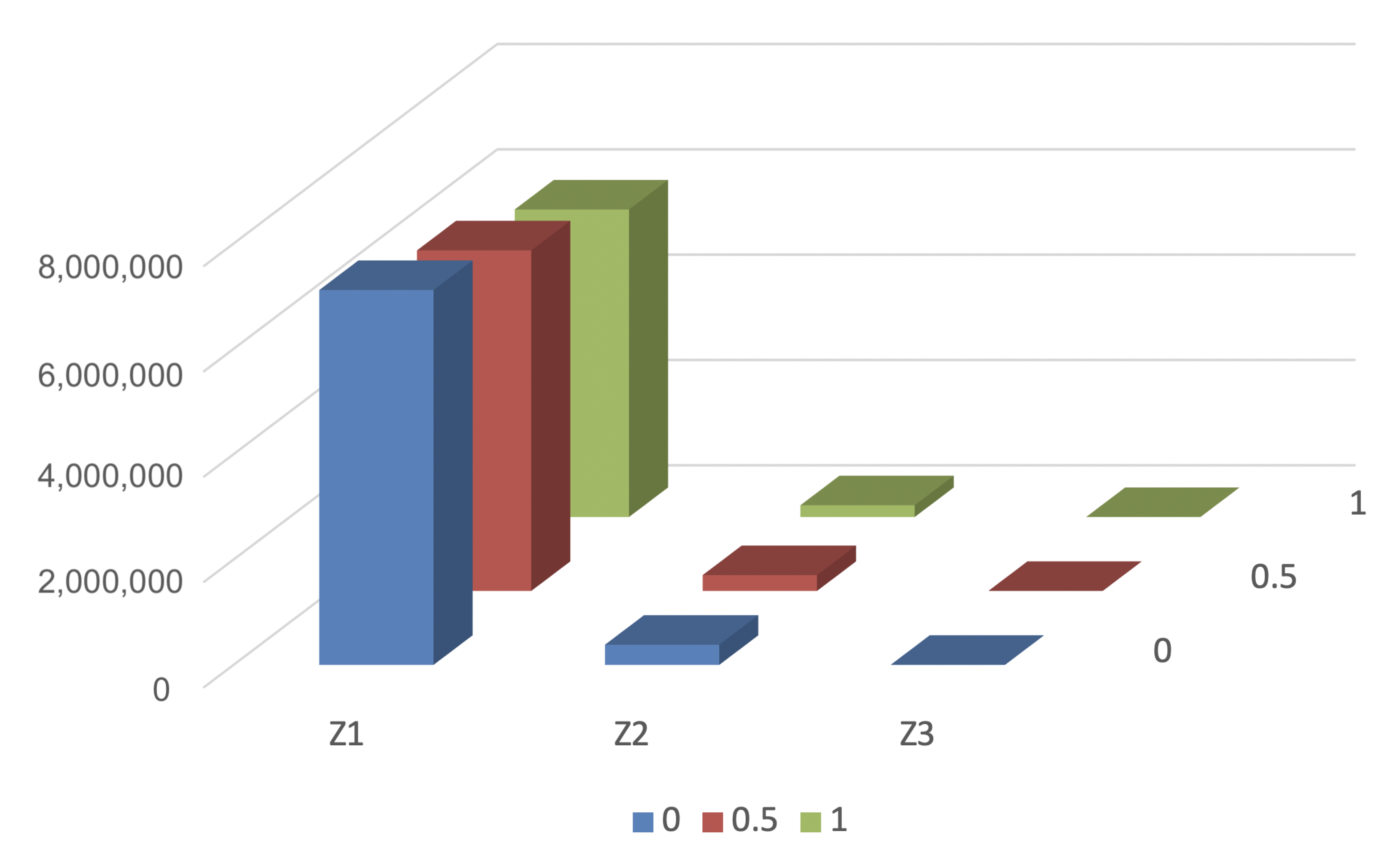
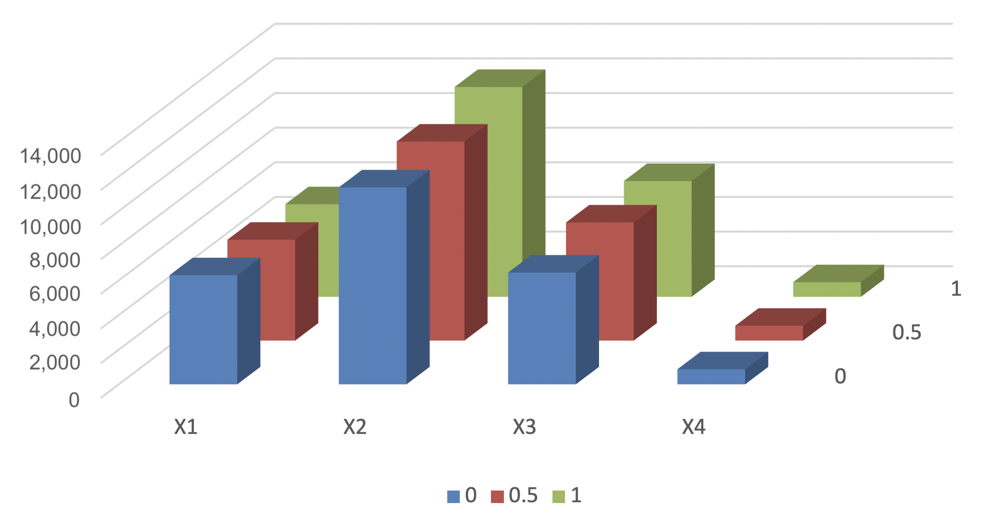
- Using values of Table 5, problem (4) of case 1 was solved using the FGP approach as defined in Section 4.2. The results obtained at the distinct value of and 1 are given in Table 8.Similarly, problems (6) and (8) of case 2 and 3 respectively were solved for the distinct value of and 1 using the FGP approach, and the result is summarized below in Table 9 and Table 10.The optimal result for various discrete choices for is presented in Table 8, Table 9 and Table 10. They show that vendor 4 has lost most of his quota due to inferior performance on the criterion set up by the manufacturer, i.e., percentage of flexibility, purchase rating, percentage of rejection, purchasing cost, and budget allocation. However, vendor 2 received more quota allocation as he performed best among the other vendors on the different performance criteria. The quota for vendor 3 is higher than the vendor 1 due to their inferior capacity. The result also indicates that if the value of increases or decreases, then the quota allocation to different vendors also starts changing consistently.
- When the demand is not fixed ( 22,000 or 23,000 or 2000 or 4000) units.
- Since the parameters are in uncertain form; we generated the optimistic, pessimistic and most likely value of the fuzzy parameters, and their corresponding solutions. The compromise solution values for , and and optimum allocation of order quantities for the vendors for the same discrete values for are summarized below in Table 8, Table 9 and Table 10.By using the values in Table 5, problem (4) of case 1 was solved using the FGP approach as defined in Section 4.2. The results obtained at the distinct value of and 1 are given in Table 11.Similarly, problem (6) and (8) of case 2 and 3 respectively were solved for the distinct value of and 1 using the FGP approach, and the result is summarized in Table 12 and Table 13.The optimal result for various discrete choices is presented in Table 11, Table 12 and Table 13. They show that vendor 4 lost most of their quota due to inferior performance on the criterion set up by the manufacturer, i.e., percentage of flexibility, purchase rating, percentage of rejection, purchasing cost, and budget allocation. However, the second vendor received more quota allocation as he performed best among the other vendors on the different performance criteria. The quota for vendor 3 is higher than the vendor 1 due to their inferior capacity. The result also indicates that if the value of increases or decreases, then the quota allocation to different vendors also starts changing consistently.
6. Result Analysis and Discussion
- Pessimistic Result ().
- From the different solutions tables and their obtained trace value, we can see that the results attained from Approach 2 are very close to the aspiration goal set by the decision-maker. Approach 2 provides a better objective value in comparison to Approach 1 for an aggregate demand of 25,000 units that yields a minimum net ordering cost of 6,837,807 rupees, minimum transportation cost of 331,160.2 rupees and a minimum late delivered units to be around 1506 (aggregated) during the process. Based on the optimization technique and the results generated from it show that the manufacturer decides to purchase 11,632 units form vendor 2, 6587 units form vendor 3, 5932 units from vendor 1 and purchase only 849 units from vendor 4 due to their most inferior performance on the criteria set (viz. the highest percentage rejections, high percentage late deliveries, less vendor rating value, less quota flexibility value, etc.).
- Most Likely Result ().
- From the different solutions tables and their obtained trace value, we can see that the results attained from Approach 1 are very close to the aspiration goal set by the decision-maker. Approach 1 provides a better objective value in comparison to Approach 2 for an aggregate demand of 25,000 units that yields a minimum net ordering cost of 6,455,521 rupees, minimum transportation cost of 298,038.7 rupees and a minimum late delivered units to be around 1328 (aggregated) during the process. Based on the optimization technique and the results generated from it, show that the manufacturer decides to purchase 11,505 units form vendor 2, 6836 units form vendor 3, 5800 units from vendor 1 and purchase only 859 units from vendor 4 due to their most inferior performance on the criteria set (viz. the highest percentage rejections, high percentage late deliveries, less vendor rating value, less quota flexibility value, etc.). (5,839,909, 224,235.7, 922.5766)
- Optimistic Result ().
- From the different solutions tables and their obtained trace value, we can see that the results attained from Approach 2 is very close to the aspiration goal set by the decision-maker. Approach 1 provides a better objective value in comparison to Approach 2 for an aggregate demand of 25,000 units that yields a minimum net ordering cost of 5,839,909 rupees, minimum transportation cost of 224,235.7 rupees and a minimum late delivered units to be around 923 (aggregated) during the process. Based on the optimization technique and the results generated from it show that the manufacturer decides to purchase 12,120 units form vendor 2, 6686 units form vendor 3, 5349 units from vendor 1 and purchase only 845 units from vendor 4 due to their most inferior performance on the criteria set (viz. the highest percentage rejections, high percentage late deliveries, less vendor rating value, less quota flexibility value, etc.). A similar conclusion can be drawn for the uncertain demand. Notable, the objective values and order quantities associated with different values do not need to be the same.
- Mean value Method.
- Since Table 6 is in the case of vagueness, where the input information is present in the form of LR fuzzy numbers. The suitable fuzzy set theory concept was applied to obtain the equivalent crisp form. Moreover, we can consider the mean method of extreme values to handle the vagueness in the input parameters. Therefore, Table 4 is revised accordingly to the mean values method, and resultant Table 14 is given below:
- The Goal Programming.
- The data given in Table 15 was used to solve the MOVSP by the goal programming approach.After using the goal programming approach, the optimal compromise solution is obtained as (6,398,528, 282,442.2, 1301.87) with the order quantities (5750,12,387,6863,0).
- The Chebyshev Goal Programming.
- The data given in Table 15 was used to solve the MOVSP by the Chebyshev goal programming approach.After using the Chebyshev goal programming approach, the optimal compromise solution is obtained as (6,439,980, 292,074.2, 1313.05) with order quantities (5750, 11, 527, 6863, 860).
- The Fuzzy Goal Programming.
- The data given in Table 15 was used to solve the MOVSP by the fuzzy goal programming approach.After using the fuzzy goal programming approach, the optimal compromise solution is obtained as (6,925,348, 297,672, 1140.43) with order quantities (4063, 16,602, 3819, 516). Also, by introducing the auxiliary variables for each objective function as , the above model is reformulated as:After using the fuzzy goal programming approach with auxiliary variables, the optimal compromise solution is obtained as (6,731,794, 299,191.8, 1088.83) with order quantities (5078, 16,590, 3332, 0).
7. Conclusions
Author Contributions
Funding
Conflicts of Interest
References
- Dickson, G.W. An analysis of vendor selection systems and decisions. J. Purch. 1966, 2, 5–17. [Google Scholar] [CrossRef]
- Dempsey, W.A. Vendor selection and the buying process. Ind. Mark. Manag. 1978, 7, 257–267. [Google Scholar] [CrossRef]
- Xia, W.; Wu, Z. Supplier selection with multiple criteria in volume discount environments. Omega 2007, 35, 494–504. [Google Scholar] [CrossRef]
- Charnes, A.; Cooper, W.W. Management Models of Industrial Applications of Linear Program; Wiley: New York, NY, USA, 1968; Volume 1–2. [Google Scholar]
- Lee, S.M. Goal Programming for Decision Analysis; Auerbach Publishers: Philadelphia, PA, USA, 1972. [Google Scholar]
- Ignizio, J.P. Goal Programming and Extensions; D.C. Heath: Lexington, KY, USA, 1976. [Google Scholar]
- Zadeh, L.A. Fuzzy Sets. Inf. Control 1965, 8, 338–353. [Google Scholar] [CrossRef]
- Zimmermann, H.J. Fuzzy Programming and Linear Programming with Several Objective Functions. Fuzzy Sets Syst. 1978, 1, 45–55. [Google Scholar] [CrossRef]
- Bellman, R.E.; Zadeh, L.A. Decision Making in a Fuzzy Environment. Manag. Sci. 1970, 17, 141–164. [Google Scholar] [CrossRef]
- Ravindran, A.R. Multiple Criteria Decision Making in Supply Chain Management; CRC Press: Boca Raton, FL, USA, 2016. [Google Scholar]
- Wind, Y.; Green, P.E.; Robinson, P.J. The determinants of vendor selection: The evaluation function approach. J. Purch. 1968, 4, 29–41. [Google Scholar] [CrossRef]
- Stewart, A.K. Vendor Rating and Credit Rating: A Comparison and Analysis. J. Purch. 1968, 4, 54–69. [Google Scholar] [CrossRef]
- Hinkle, C.L.; Robinson, P.J.; Green, P.E. Vendor evaluation using cluster analysis. J. Purch. 1969, 5, 49–58. [Google Scholar] [CrossRef]
- Miller, W.G. Selection Criteria for Computer System Adoption. In The Educational Technology Reviews Series, Number Nine, The Computer and Education; Educational Technology Publications: Englewood Cliffs, NJ, USA, 1973; pp. 118–122. [Google Scholar]
- McMillan, J.R. The Role of Perceived Risk in Vendor Selection Decisions. Ph.D. Thesis, The Ohio State University, Columbus, OH, USA, 1972. [Google Scholar]
- Lucas, H.; Moore, J. A multiple-criterion scoring approach to information system project selection. INFOR Inf. Syst. Oper. Res. 1976, 14, 1–12. [Google Scholar] [CrossRef]
- Wieters, C.D.; Ostrom, L.L. Supplier evaluation as a new marketing tool. Ind. Mark. Manag. 1979, 8, 161–166. [Google Scholar] [CrossRef]
- Manzer, L.L.; Ireland, R.D.; Van Auken, P.M. A matrix approach to vendor selection for small business buyers. Am. J. Small Bus. 1980, 4, 21–28. [Google Scholar] [CrossRef]
- Fakhrzad, M.B.; Goodarzian, F. A fuzzy multi-objective programming approach to develop a green closed-loop supply chain network design problem under uncertainty: Modifications of the imperialist competitive algorithm. RAIRO-Oper. Res. 2019, 53, 963–990. [Google Scholar] [CrossRef]
- Goodarzian, F.; Hosseini-Nasab, H.; Munuzuri, J.; Fakhrzad, M.B. A multi-objective pharmaceutical supply chain network based on a robust fuzzy model: A comparison of meta-heuristics. Appl. Soft Comput. J. 2020, 92, 106331. [Google Scholar] [CrossRef]
- Goodarzian, F.; Hosseini-Nasab, H. Applying a fuzzy multi-objective model for a production-distribution network design problem by using a novel self-adoptive evolutionary algorithm. Int. J. Syst. Sci. Oper. Logist. 2019. [Google Scholar] [CrossRef]
- Huang, L.; Murong, L.; Wang, W. Green closed-loop supply chain network design considering cost control and CO2 emission. Mod. Supply Chain. Res. Appl. 2020, 2, 42–59. [Google Scholar] [CrossRef]
- Kumar, M.; Vrat, P.; Shankar, R. A fuzzy programming approach for vendor selection problem in a supply chain. Int. J. Prod. Econ. 2006, 101, 273–285. [Google Scholar] [CrossRef]
- Weber, C.A.; Current, J.R. Theory and methodology: A multi-objective approach to vendor selection. Eur. J. Oper. Res. 1993, 68, 173–184. [Google Scholar] [CrossRef]
- Dahel, N.E. Vendor selection and order quantity allocation in volume discount environments. Supply Chain Manag. An Int. J. 2003, 8, 335–342. [Google Scholar] [CrossRef]
- Pokharel, S. A two objective model for decision making in a supply chain. Int. J. Prod. Econ. 2008, 111, 378–388. [Google Scholar] [CrossRef]
- Tsai, W.C.; Wang, C.H. Decision making of sourcing and order allocation with price discounts. J. Manuf. Syst. 2010, 29, 47–54. [Google Scholar] [CrossRef]
- Rezaei, J.; Davoodi, M. Multi-objective models for lot-sizing with supplier selection. Int. J. Prod. Econ. 2011, 130, 77–86. [Google Scholar] [CrossRef]
- Kumar, M.; Vrat, P.; Shankar, R. A fuzzy goal programming approach for vendor selection problem in a supply chain. Comput. Ind. Eng. 2004, 46, 69–85. [Google Scholar] [CrossRef]
- Lamberson, L.R.; Diederich, D.; Wuori, J. Quantitative vendor evaluation. J. Purch. Mater. Manag. 1976, 12, 19–28. [Google Scholar] [CrossRef]
- Kumar, A.; Karunamoorthy, N.; Anand, L.S.; Babu, T.R. Linear approach for solving a piecewise linear vendor selection problem of quantity discounts using lexicographic method. Int. J. Adv. Manuf. Technol. 2006, 28, 1254–1260. [Google Scholar]
- Amid, A.; Ghodsypour, S.H.; O’Brien, C. Fuzzy multiobjective linear model for supplier selection in a supply chain. Int. J. Prod. Econ. 2006, 104, 394–407. [Google Scholar] [CrossRef]
- Amid, A.; Ghodsypour, S.H.; O’Brien, C. A weighted additive fuzzy multiobjective model for the supplier selection problem under price breaks in a supply chain. Int. J. Prod. Econ. 2009, 121, 323–332. [Google Scholar] [CrossRef]
- Tiwari, R.N.; Dharmar, S.; Rao, J.R. Fuzzy goal programming—An additive model. Fuzzy Sets Syst. 1987, 24, 27–34. [Google Scholar] [CrossRef]
- Lin, C.C. A weighted max–min model for fuzzy goal programming. Fuzzy Sets Syst. 2004, 142, 407–420. [Google Scholar] [CrossRef]
- Amid, A.; Ghodsypour, S.H.; O’Brien, C. A weighted max–min model for fuzzy multi-objective supplier selection in a supply chain. Int. J. Prod. Econ. 2011, 131, 139–145. [Google Scholar] [CrossRef]
- Liao, C.N.; Kao, H.P. Supplier selection model using Taguchi loss function, analytical hierarchy process and multi-choice goal programming. Comput. Ind. Eng. 2010, 58, 571–577. [Google Scholar] [CrossRef]
- Liao, C.N.; Kao, H.P. An integrated fuzzy TOPSIS and MCGP approach to supplier selection in supply chain management. Expert Syst. Appl. 2011, 38, 10803–10811. [Google Scholar] [CrossRef]
- Wu, D.D.; Zhang, Y.; Wu, D.; Olson, D.L. Fuzzy multi-objective programming for supplier selection and risk modeling: A possibility approach. Eur. J. Oper. Res. 2010, 200, 774–787. [Google Scholar] [CrossRef]
- Ozkok, B.A.; Tiryaki, F. A compensatory fuzzy approach to multi-objective linear supplier selection problem with multiple-item. Expert Syst. Appl. 2011, 38, 11363–11368. [Google Scholar] [CrossRef]
- Pandey, P.; Shah, B.J.; Gajjar, H. A fuzzy goal programming approach for selecting sustainable suppliers. Benchmarking An Int. J. 2017, 24, 1138–1165. [Google Scholar] [CrossRef]
- Mirzaee, H.; Naderi, B.; Pasandideh, S.H.R. A preemptive fuzzy goal programming model for generalized supplier selection and order allocation with incremental discount. Comput. Ind. Eng. 2018, 122, 292–302. [Google Scholar] [CrossRef]
- Abbas, Y.A.S. Enhancement fuzzy goal programming approach for multi-item/multi-supplier selection problem ina fuzzy environment. Int. J. Dev. Res. 2018, 8, 23521–23530. [Google Scholar]
- Sari, I.U. Development of an integrated discounting strategy based on vendors’ expectations using FAHP and fuzzy goal programming. Technol. Econ. Dev. Econ. 2018, 24, 635–652. [Google Scholar] [CrossRef]
- Wadhwa, V. Multi-Objective Multi-Period Supplier Selection Problem with Product Bundling. In Multiple Criteria Decision Making in Supply Chain Management; CRC Press: Boca Raton, FL, USA, 2017; pp. 285–310. [Google Scholar]
- Kamal, M.; Gupta, S.; Raina, A.A. Fuzzy multi-objective supplier selection problem in a supply chain. World Sci. News 2018, 100, 165–183. [Google Scholar]
- Shaw, K. Fuzzy multi-objective, multi-item, multi-supplier, lot-sizing considering carbon footprint. Int. J. Math. Oper. Res. 2017, 11, 171–203. [Google Scholar] [CrossRef]
- Aggarwal, R.; Singh, S.P.; Kapur, P. Integrated dynamic vendor selection and order allocation problem for the time dependent and stochastic data. Benchmarking An Int. J. 2018, 25, 777–796. [Google Scholar] [CrossRef]
- Islam, S.; Deb, S.C. Neutrosophic Goal Programming Approach to A Green Supplier Selection Model with Quantity Discount. Neutrosophic Sets Syst. 2019, 30, 98–112. [Google Scholar]
- Ho, H.P. The supplier selection problem of a manufacturing company using the weighted multi-choice goal programming and MINMAX multi-choice goal programming. Appl. Math. Model. 2019, 75, 819–836. [Google Scholar] [CrossRef]
- Torres-Ruiz, A.; Ravindran, A.R. Use of interval data envelopment analysis, goal programming and dynamic eco-efficiency assessment for sustainable supplier management. Comput. Ind. Eng. 2019, 131, 211–226. [Google Scholar] [CrossRef]
- Hassan, M.M.; Jiang, D.; Ullah, A.S.; Noor-E-Alam, M. Resilient Supplier Selection in Logistic 4.0: An integrated approach of Fuzzy Multi-Attribute Decision Making (F-MADM) and Multi-choice Goal Programming (MCGP) with Heterogeneous. arXiv 2019, arXiv:1904.09837. [Google Scholar]
- Alizadeh, A.; Yousefi, S. An integrated Taguchi loss function–fuzzy cognitive map–MCGP with utility function approach for supplier selection problem. Neural Comput. Appl. 2019, 31, 7595–7614. [Google Scholar] [CrossRef]
- Ozkan, O.; Aydin, S. Supplier Selection with Intuitionistic Fuzzy AHP and Goal Programming. In International Conference on Intelligent and Fuzzy Systems, Proceedings of the INFUS 2019: Intelligent and Fuzzy Techniques in Big Data Analytics and Decision Making, Istanbul, Turkey, 23–25 July 2019; Springer: Berlin/Heidelberg, Germany, 2019; pp. 835–842. [Google Scholar]
- Jia, R.; Liu, Y.; Bai, X. Sustainable supplier selection and order allocation: Distributionally robust goal programming model and tractable approximation. Comput. Ind. Eng. 2020, 140, 106267. [Google Scholar] [CrossRef]
- Krishankumar, R.; Ravichandran, K.S.; Tyagi, S.K. Solving cloud vendor selection problem using intuitionistic fuzzy decision framework. Neural Comput. Appl. 2020, 32, 589–602. [Google Scholar] [CrossRef]
- Arikan, F. A fuzzy solution approach for multi objective supplier selection. Expert Syst. Appl. 2013, 40, 947–952. [Google Scholar] [CrossRef]
- Lai, Y.J.; Hwang, C.L. Possibilistic linear programming for managing interest rate risk. Fuzzy Sets Syst. 1993, 54, 135–146. [Google Scholar] [CrossRef]
- Lai, Y.J.; Hwang, C.L. Fuzzy multiple objective decision making. In Fuzzy Multiple Objective Decision Making; Springer: Berlin/Heidelberg, Germany, 1994; pp. 139–262. [Google Scholar]
- Shirkouhi, N.; Shakouri, S.; Javadi, B.; Keramati, A. Supplier selection and order allocation problem using a two-phase fuzzy multi-objective linear programming. Appl. Math. Model. 2013, 37, 9308–9323. [Google Scholar] [CrossRef]
- Kilic, H.S. An integrated approach for supplier selection in multi-item/multi-supplier environment. Appl. Math. Model. 2013, 37, 7752–7763. [Google Scholar] [CrossRef]
- Rouyendegh, B.D.; Saputro, T.E. Supplier selection using integrated fuzzy TOPSIS and MCGP: A case study. Procedia-Soc. Behav. Sci. 2014, 116, 3957–3970. [Google Scholar] [CrossRef]
- Jadidi, O.M.I.D.; Zolfaghari, S.; Cavalieri, S. A new normalized goal programming model for multi-objective problems: A case of supplier selection and order allocation. Int. J. Prod. Econ. 2014, 148, 158–165. [Google Scholar] [CrossRef]
- Chang, C.T.; Ku, C.Y.; Ho, H.P. Fuzzy multi-choice goal programming for supplier selection. Int. J. Oper. Res. Inf. Syst. 2010, 1, 28–52. [Google Scholar] [CrossRef][Green Version]
- Karimi, H.; Rezaeinia, A. Supplier selection using revised multi-segment goal programming model. Int. J. Adv. Manuf. Technol. 2014, 70, 1227–1234. [Google Scholar] [CrossRef]
- Sivrikaya, B.T.; Kaya, A.; Dursun, E.; Cebi, F. Fuzzy AHP-goal programming approach for a supplier selection problem. Res. Logist. Prod. 2015, 5, 271–285. [Google Scholar]
- Tirkolaee, E.B.; Mardani, A.; Dashtian, Z.; Soltani, M.; Weber, G.W. A novel hybrid method using fuzzy decision making and multi-objective programming for sustainable-reliable supplier selection in two-echelon supply chain design. J. Clean. Prod. 2020, 250, 119517. [Google Scholar] [CrossRef]
- Maragatham, M.; Jiji, D.S.; Mariappan, P. A Fuzzy Integer Programming Approach for Vendor Selection Problem. Our Herit. 2020, 68, 57–64. [Google Scholar]
- Sumrit, D. Supplier selection for vendor-managed inventory in healthcare using fuzzy multi-criteria decision-making approach. Decis. Sci. Lett. 2020, 9, 233–256. [Google Scholar] [CrossRef]
- Shen, C.W.; Peng, Y.T.; Tu, C.S. Multi-Criteria Decision-Making Techniques for Solving the Airport Ground Handling Service Equipment Vendor Selection Problem. Sustainability 2019, 11, 3466. [Google Scholar] [CrossRef]
- Charles, V.; Gupta, S.; Ali, I. A Fuzzy Goal Programming Approach for Solving Multi-Objective Supply Chain Network Problems with Pareto-Distributed Random Variables. Int. J. Uncertain. Fuzziness-Knowl.-Based Syst. 2019, 27, 559–593. [Google Scholar] [CrossRef]
- Razmi, J.; Jafarian, E.; Amin, S.H. An intuitionistic fuzzy goal programming approach for finding pareto-optimal solutions to multi-objective programming problems. Expert Syst. Appl. 2016, 65, 181–193. [Google Scholar] [CrossRef]
- Yong, D. Plant location selection based on fuzzy TOPSIS. Int. J. Adv. Manuf. Technol. 2006, 7–8, 839–844. [Google Scholar] [CrossRef]
- Dulmin, R.; Mininno, V. Supplier selection using a multi-criteria decision aid method. J. Purch. Supply Manag. 2003, 9, 177–187. [Google Scholar] [CrossRef]
- Tam, M.C.; Tummala, V.R. An application of the AHP in vendor selection of a telecommunications system. Omega 2001, 29, 171–182. [Google Scholar] [CrossRef]
- Muralidharan, C.; Anantharaman, N.; Deshmukh, S. Vendor rating in purchasing scenario: A confidence interval approach. Int. J. Oper. Prod. Manag. 2001, 21, 1305–1326. [Google Scholar] [CrossRef]
- Petroni, A.; Braglia, M. Vendor selection using principal component analysis. J. Supply Chain Manag. 2000, 36, 63–69. [Google Scholar] [CrossRef]
- Yahya, S.; Kingsman, B. Vendor rating for an entrepreneur development programme: A case study using the analytic hierarchy process method. J. Oper. Res. Soc. 1999, 50, 916–930. [Google Scholar] [CrossRef]
- Mandal, A.; Deshmukh, S. Vendor selection using interpretive structural modelling (ISM). Int. J. Oper. Prod. Manag. 1994, 14, 52–59. [Google Scholar] [CrossRef]
- Abbasbandy, S.; Asady, B. The nearest trapezoidal fuzzy number to a fuzzy quantity. Appl. Math. Comput. 2004, 156, 381–386. [Google Scholar] [CrossRef]
- Bede, B. Mathematics of Fuzzy Sets and Fuzzy Logic; Springer: Berlin/Heidelberg, Germany, 2013. [Google Scholar]
- Zimmermann, H.J. Fuzzy Sets Theory and Its Applications; Kluwer: Boston, MA, USA, 1991. [Google Scholar]


| Authors | Model Objectives | Techniques Used | Converted to Single Objective By |
|---|---|---|---|
| Jia et al. [55] | Multiple | Preemtive GP | Expected & join chance constraints |
| Tirkolaee et al. [67] | Multiple | FANP,FTOPSIS & FDEMATEL | WGP |
| Maragatham et al. [68] | Multiple | FILP | Modefied Zimmermann’s approach |
| Sumrit [69] | Multiple | Fuzzy Delphi, Fuzzy SWARA | MCDM framewoek proposed |
| Shen et al. [70] | Single | Fuzzy TOPSIS | MCGP |
| Mahmudul Hassan et al. [52] | Multi-Attribute | FTOPSIS | MCGP |
| Alizadeh and Yousefi [53] | Multiple | MCGP | Utility Function |
| Ozkan and Aydin [54] | Multiple | IFAHP | FGP |
| Islam and Deb [49] | Multiple | Neutrosophic AHP & GP | Compared with FGP |
| Ho [50] | Multiple | WGP, FG | WGP, MINMAX MCGP |
| Torres-Ruiz and Ravindran [51] | Multiple | Preemtive, Non-preemtive & FGP | DEA |
| Mirzaee et al. [42] | Multiple | MILP | Preemtive & WFP, Max-min & Classical GP |
| Abbas [43] | Multiple | Intractive Fuzzy GP | Alpha-cut, FGP |
| Sari [44] | Multiple | FAHP, FGP | FGP |
| Kamal et al. [46] | Multiple | WFGP | Weighted root power mean, linear, exponential, & hyperbolic |
| Charles et al. [71] | Multiple | Additive, Weighted & Preemtive GP | FGP |
| Aggarwal et al. [48] | Multiple | Non-preemtive GP | Weighted Sum AOF |
| Shaw [47] | Multiple | IGP,WGP, IFG | Interactive fuzzy -constraint |
| Wadhwa [45] | Multiple Criteria | FGP, Tcebycheff Min-max | Preemtive & non-preemtive GP |
| Pandey et al. [41] | Multiple | WFGP | Hyperbolic membership function |
| Razmi et al. [72] | Multiple | IFGP | Two-step GP |
| Sivrikaya et al. [66] | Multiple | FAHP, GP | Trapezoidal Fuzzy, geometric mean Method |
| Jadidi et al. [63] | Multiple | WGP, TOPSIS, Min-Max GP, WMin-Max, | Compromise Programming, Normalized GP developed |
| Karimi and Rezaeinia [65] | Multiple | multi-segment goal programming | multi-segment goal programming revised |
| Rouyendegh and Saputro [62] | Multi-Criteria | FTOPSIS, MCGP | Triangular fuzzy numbers |
| Arikan [57] | Multiple | FGP | Fuzzy additive, augumented max-min model |
| Shirkouhi et al. [60] | Multiple | FMOLP | Piecewise linear membership |
| Kilic [61] | Multiple | FTOPSIS & MILP | Many MCDM proposed |
| Ozkok and Tiryaki [40] | Multi-item | MLSSP-MI | Fuzzy operator |
| Ozkok and Tiryaki [40] | Multiple | Weners’ fuzzy and operator | compensatory fuzzy approach developed |
| Rezaei and Davoodi [28] | Multiple | Genatic Algorithm | Two Multiobjective Mixed-Integer Non-linear models developed |
| Authors | Model Objectives | Techniques Used | Converted to Single Objective by |
|---|---|---|---|
| Chang et al. [64] | Multiple | MCGP | FMCGP |
| Liao and Kao [37], Liao and Kao [38] | Multi-Criteria | AHP, Taguschi loss function, FTOPSIS | MCGP |
| Wu et al. [39] | Multiple | FMOP | Simulation |
| Amid et al. [32], Amid et al. [33], Amid et al. [36] | Multiple | Fuzzy-assymetric | weighted additive, alpha-cute approach |
| Pokharel [26] | Two Objectives | STEP Method | MOP |
| Xia and Wu [3] | Multi-Criteria | AHP | MILP |
| Yong [73] | Multi-Criteria | Fuzzy TOPSIS | new FTOPSIS proposed |
| Kumar et al. [23], Kumar et al. [29] | Multiple | Fuzzy Integer | Linear membership |
| Lin [35] | Multiple | FGP | Weighted Max-min |
| Dulmin and Mininno [74] | Multiple criteria | promethee/gaia techniques | MCDM investigated |
| Tam and Tummala [75] | Multi-Criteria | AHP | AHP-based model developed |
| Muralidharan et al. [76] | Multiple-Criteria | Confidence interval approach | Ranking methodology proposed |
| Petroni and Braglia [77] | Multi-Attribute | PCA | Multi-attribute approach discussed |
| Yahya and Kingsman [78] | Multiple criteria | AHP | Vendor rating and comparison |
| Mandal and Deshmukh [79] | Qualitative research | Interpretive Structural Modeling | Vendor selection framework |
| Lai and Hwang [58] | Single | Probalistic LP | Augmented max-min proposed |
| Weber and Current [24] | Multi-criteria | ILP | IMB XT |
| Tiwari et al. [34] | Multiple | aditive & weighted GP | additive FGP formulated |
| Indices | |
|---|---|
| j | vendor’s index, ∀ |
| k | objectives index, ∀ |
| Parameters | |
| n | vendors’ number who are competing for selection |
| D | aggregate item demand for a fixed planning period |
| per unit item price for the quantity ordered to the vendor | |
| unit item transportation cost from the vendor | |
| percentage for the late delivered units by the vendor | |
| upper limit for the vendor’s quantity available | |
| each vendor’s budget constraint allocation | |
| percentage for the vendor rejected units | |
| rating value for the vendor | |
| P | vendor’s minimum total purchasing value |
| vendor quota flexibility | |
| F | vendor’s minimum value flexible in supply quota |
| R | maximum affordable rejection by a purchaser |
| Decision Variable | |
| order quantity is given to the vendor j |
| Vendors | 1 | 2 | 3 | 4 |
|---|---|---|---|---|
| (110, 130, 10, 15) | (305, 325, 15, 20) | (250, 265, 13, 18) | (355, 370, 12, 20) | |
| (15, 17, 2, 3) | (11, 12, 1, 2) | (5, 7, 0.9, 1.8) | (21, 24, 4, 6) | |
| (2, 2.5, 0.3, 0.7) | (3, 4.5, 0.6, 0.9) | (9, 11, 0.8, 1.1) | (4, 6, 0.5, 0.7) | |
| (5600, 5800, 200, 400) | (16,500, 16,900, 600, 750) | (7000, 7900, 250, 450) | (5500, 5800, 310, 420) | |
| (1,250,000, 1,300,000, 50,000, 60,000) | (5,000,000, 5,500,000, 65,000, 70,000) | (1,750,000, 1,800,000, 40,000, 45,000) | (300,000, 325,000, 10,000, 15,000) | |
| (4, 6, 0.8, 1.2) | (4, 5.5, 0.6, 0.8) | (1, 2, 0.1, 0.2) | (7.5, 8.5, 1.5, 1.8) | |
| (0.05, 0.06, 0.001, 0.002) | (0.02, 0.03, 0.002, 0.003) | (0.07, 0.09, 0.001, 0.003) | (0.03, 0.04, 0.001, 0.002) | |
| (0.87, 0.88, 0.01, 0.02) | (0.90, 0.94, 0.04, 0.06) | (0.91, 0.93, 0.03, 0.05) | (0.89, 0.90, 0.08, 0.09) |
| Vendors | 1 | 2 | 3 | 4 | |
|---|---|---|---|---|---|
| 0 | 145.00 | 345.00 | 283.00 | 390.00 | |
| 0.5 | 122.50 | 317.50 | 260.00 | 366.50 | |
| 1 | 100.00 | 290.00 | 237.00 | 343.00 | |
| 0 | 20.00 | 14.00 | 8.80 | 30.00 | |
| 0.5 | 16.50 | 12.00 | 6.45 | 23.50 | |
| 1 | 13.00 | 10.00 | 4.10 | 17.00 | |
| 0 | 3.2 | 5.4 | 12.10 | 6.70 | |
| 0.5 | 2.45 | 3.9 | 10.15 | 5.10 | |
| 1 | 1.7 | 2.4 | 8.20 | 3.50 | |
| 0 | 6200 | 17,650 | 8350 | 6220 | |
| 0.5 | 5800 | 16,775 | 7550 | 5705 | |
| 1 | 5400 | 15,900 | 6750 | 5190 | |
| 0 | 1,360,000 | 5,570,000 | 1,845,000 | 340,000 | |
| 0.5 | 1,280,000 | 5,252,500 | 1,777,500 | 315,000 | |
| 1 | 1,200,000 | 4,935,000 | 1,710,000 | 290,000 | |
| 0 | 7.20 | 6.30 | 2.20 | 10.30 | |
| 0.5 | 5.20 | 4.85 | 1.55 | 8.15 | |
| 1 | 3.20 | 3.40 | 0.90 | 6.00 | |
| 0 | 0.0620 | 0.0330 | 0.0930 | 0.0420 | |
| 0.5 | 0.0555 | 0.0255 | 0.0810 | 0.0355 | |
| 1 | 0.0490 | 0.0180 | 0.0690 | 0.0290 | |
| 0 | 0.90 | 1.00 | 0.98 | 0.99 | |
| 0.5 | 0.88 | 0.93 | 0.93 | 0.90 | |
| 1 | 0.86 | 0.86 | 0.88 | 0.81 |
| Vendors | 1 | 2 | 3 | 4 | |
|---|---|---|---|---|---|
| 0 | 148.79 | 350.00 | 287.55 | 395.06 | |
| 0.5 | 123.13 | 318.13 | 260.63 | 367.52 | |
| 1 | 97.46 | 286.20 | 233.71 | 339.96 | |
| 0 | 20.76 | 14.51 | 9.25 | 31.52 | |
| 0.5 | 16.62 | 12.13 | 6.56 | 23.75 | |
| 1 | 12.49 | 9.74 | 3.87 | 15.98 | |
| 0 | 3.37 | 5.63 | 12.38 | 6.87 | |
| 0.5 | 2.50 | 3.94 | 10.18 | 5.13 | |
| 1 | 1.63 | 2.25 | 7.99 | 3.37 | |
| 0 | 6301 | 17,840 | 8464 | 6326 | |
| 0.5 | 5825 | 16,794 | 7575 | 5719 | |
| 1 | 5349 | 15,748 | 6687 | 5111 | |
| 0 | 1,375,198 | 5,587,731 | 1,856,398 | 343,799 | |
| 0.5 | 1,281,266 | 5,253,133 | 1,778,133 | 315,633 | |
| 1 | 1,187,335 | 4,918,536 | 1,699,868 | 287,467 | |
| 0 | 7.51 | 6.51 | 2.25 | 10.75 | |
| 0.5 | 5.25 | 4.87 | 1.56 | 8.18 | |
| 1 | 2.99 | 3.25 | 0.87 | 5.62 | |
| 0 | 0.0625 | 0.0337 | 0.0937 | 0.0425 | |
| 0.5 | 0.0556 | 0.0256 | 0.0813 | 0.0356 | |
| 1 | 0.0487 | 0.0174 | 0.0687 | 0.0287 | |
| 0 | 0.91 | 1.02 | 0.99 | 1.02 | |
| 0.5 | 0.88 | 0.93 | 0.93 | 0.91 | |
| 1 | 0.86 | 0.85 | 0.87 | 0.79 |
| Vendors | 1 | 2 | 3 | 4 | |
|---|---|---|---|---|---|
| 0 | 135.43 | 338.22 | 269.79 | 380.63 | |
| 0.5 | 123.64 | 322.73 | 257.18 | 368.69 | |
| 1 | 111.85 | 307.24 | 244.57 | 356.75 | |
| 0 | 17.82 | 13.15 | 7.52 | 27.04 | |
| 0.5 | 16.39 | 11.88 | 6.18 | 23.06 | |
| 1 | 14.96 | 10.61 | 4.84 | 19.08 | |
| 0 | 2.93 | 4.88 | 10.84 | 5.99 | |
| 0.5 | 2.48 | 3.87 | 9.61 | 4.98 | |
| 1 | 2.03 | 2.86 | 8.38 | 3.97 | |
| 0 | 5932 | 17,230 | 7885 | 6043 | |
| 0.5 | 5700 | 16,817 | 7505 | 5689 | |
| 1 | 5468 | 16,403 | 7124 | 5335 | |
| 0 | 1,331,185 | 5,394,682 | 1,777,112 | 323,239 | |
| 0.5 | 1,280,245 | 5,231,522 | 1,764,536 | 308,615 | |
| 1 | 1,229,305 | 5,068,362 | 1,751,960 | 293,990 | |
| 0 | 6.44 | 5.61 | 1.87 | 8.67 | |
| 0.5 | 5.51 | 4.63 | 1.49 | 7.54 | |
| 1 | 4.58 | 3.65 | 1.11 | 6.41 | |
| 0 | 0.0605 | 0.0286 | 0.0875 | 0.0395 | |
| 0.5 | 0.0547 | 0.0246 | 0.0794 | 0.0357 | |
| 1 | 0.0488 | 0.0206 | 0.0714 | 0.0319 | |
| 0 | 0.88 | 0.95 | 0.96 | 0.91 | |
| 0.5 | 0.87 | 0.92 | 0.94 | 0.88 | |
| 1 | 0.85 | 0.88 | 0.91 | 0.84 |
| Objective Value | Vendor’s Allocation | |
|---|---|---|
| 0 | (7,232,987, 385,099.2, 1431.551) | (6200, 14,845, 6084, 871) |
| 0.5 | (6,455,521, 298,038.7, 1328.458) | (5800, 11,505, 6836, 859) |
| 1 | (5,911,035, 232,290, 962.99) | (5400, 122,005, 6750, 845) |
| Objective Value | Vendor’s Allocation | |
|---|---|---|
| 0 | (7,118,268, 382,976.7, 1674.064) | (6301, 11,374, 6455, 870) |
| 0.5 | (6,467,487, 301,375.7, 1337.023) | (5825, 11,495, 6822, 858) |
| 1 | (5,839,909, 224,235.7, 922.5766) | (5349, 12,120, 6686, 845) |
| Objective Value | Vendor’s Allocation | |
|---|---|---|
| 0 | (6,837,807, 331,160.2, 1506.335) | (5932, 11,632, 6587, 849) |
| 0.5 | (6,522,167, 292,957, 1055.71) | (5700, 11,602, 6861, 837) |
| 1 | (6,206,943, 254,909.6, 1072.01) | (5468, 11,584, 7124, 824) |
| Objective Value | Vendor’s Allocation | |
|---|---|---|
| 0 | (7,710,017, 395,237.2, 1769.69) | (6200, 13,410, 6519, 871) |
| 0.5 | (5,979,271, 280,038.7, 1269.95) | (5800, 10,005, 6836, 859) |
| 1 | (4,461,035, 182,290, 842.99) | (5400, 7005, 6750, 845) |
| Objective Value | Vendor’s Allocation | |
|---|---|---|
| 0 | (8,172,818, 426,695.3, 1833.757) | (6301, 14,387, 6455, 870) |
| 0.5 | (6,070,779, 286,249.6, 1287.89) | (5825, 10,248, 6822, 858) |
| 1 | (4,263,805, 170,597.5, 798.66) | (5349, 6613, 6686, 845) |
| Objective Value | Vendor’s Allocation | |
|---|---|---|
| 0 | (6,866,894, 332,291.1, 1510.53) | (5932, 11,718, 6587, 849) |
| 0.5 | (5,788,602, 265,953.7, 990.71) | (5700, 9329, 6861, 837) |
| 1 | (4,784,421, 205,785.3, 939.58) | (5468, 6954, 7124, 824) |
| Vendors | 1 | 2 | 3 | 4 |
|---|---|---|---|---|
| 122.50 | 316.30 | 258.80 | 364.50 | |
| 16.30 | 11.80 | 6.20 | 23.00 | |
| 2.35 | 3.825 | 10.075 | 5.05 | |
| 5750 | 16,737 | 7500 | 5678 | |
| 1,277,500 | 5,251,250 | 1,776,250 | ||
| 5.10 | 4.80 | 1.525 | 8.075 | |
| 0.055 | 0.025 | 0.081 | 0.035 | |
| 0.878 | 0.925 | 0.925 | 0.898 |
| Problem 1(a) of case 1 | |||
|---|---|---|---|
| 0 | 7,619,517.75 | 7,502,918.76 | 1.0155 |
| 0.5 | 6,754,888.16 | 6,770,199.72 | 0.9977 |
| 1 | 6,144,287.99 | 6,065,067.28 | 1.0131 |
| Problem 1(a) of case 2 | |||
| 0 | 7,619,517.75 | 7,170,473.54 | 1.0626 |
| 0.5 | 6,754,888.16 | 6,816,179.71 | 0.9910 |
| 1 | 6,144,287.99 | 6,462,924.61 | 0.9506 |
| Problem 1(a) of case 3 | |||
| 0 | 7,502,918.76 | 7,170,473.54 | 1.0464 |
| 0.5 | 6,770,199.72 | 6,816,179.71 | 0.9934 |
| 1 | 6,065,067.28 | 6,462,924.61 | 0.9384 |
© 2020 by the authors. Licensee MDPI, Basel, Switzerland. This article is an open access article distributed under the terms and conditions of the Creative Commons Attribution (CC BY) license (http://creativecommons.org/licenses/by/4.0/).
Share and Cite
Ali, I.; Fügenschuh, A.; Gupta, S.; Modibbo, U.M. The LR-Type Fuzzy Multi-Objective Vendor Selection Problem in Supply Chain Management. Mathematics 2020, 8, 1621. https://doi.org/10.3390/math8091621
Ali I, Fügenschuh A, Gupta S, Modibbo UM. The LR-Type Fuzzy Multi-Objective Vendor Selection Problem in Supply Chain Management. Mathematics. 2020; 8(9):1621. https://doi.org/10.3390/math8091621
Chicago/Turabian StyleAli, Irfan, Armin Fügenschuh, Srikant Gupta, and Umar Muhammad Modibbo. 2020. "The LR-Type Fuzzy Multi-Objective Vendor Selection Problem in Supply Chain Management" Mathematics 8, no. 9: 1621. https://doi.org/10.3390/math8091621
APA StyleAli, I., Fügenschuh, A., Gupta, S., & Modibbo, U. M. (2020). The LR-Type Fuzzy Multi-Objective Vendor Selection Problem in Supply Chain Management. Mathematics, 8(9), 1621. https://doi.org/10.3390/math8091621