Article

A New Extended Two-Parameter Distribution: Properties, Estimation Methods, and Applications in Medicine and Geology

1
Department of Mathematics, Tafila Technical University, Tafila 66110, Jordan
2
Department of Statistics, Mathematics and Insurance, Benha University, Benha 13511, Egypt
3
Institute for Mathematical Research, Universiti Putra Malaysia, Selangor 43400, Malaysia
*
Author to whom correspondence should be addressed.
Mathematics 2020, 8(9), 1578; https://doi.org/10.3390/math8091578
Submission received: 20 July 2020 / Revised: 7 August 2020 / Accepted: 11 August 2020 / Published: 12 September 2020
(This article belongs to the Special Issue Probability, Statistics and Their Applications)

Abstract

:
In this paper, a new two-parameter generalized Ramos–Louzada distribution is proposed. The proposed model provides more flexibility in modeling data with increasing, decreasing, J-shaped, and reversed-J shaped hazard rate functions. Several statistical properties of the model were derived. The unknown parameters of the new distribution were explored using eight frequentist estimation approaches. These approaches are important for developing guidelines to choose the best method of estimation for the model parameters, which would be of great interest to practitioners and applied statisticians. Detailed numerical simulations are presented to examine the bias and the mean square error of the proposed estimators. The best estimation method and ordering performance of the estimators were determined using the partial and overall ranks of all estimation methods for various parameter combinations. The performance of the proposed distribution is illustrated using two real datasets from the fields of medicine and geology, and both datasets show that the new model is more appropriate as compared to the Marshall–Olkin exponential, exponentiated exponential, beta exponential, gamma, Poisson–Lomax, Lindley geometric, generalized Lindley, and Lindley distributions, among others.

1. Introduction

Probability distributions have great importance for modeling data in several areas, such as medicine, engineering, and life testing, among others. Ramos and Louzada [1] recently introduced a one-parameter distribution called the Ramos–Louzada (RL) distribution with survival function (SF) given by
S ( t | λ ) = 1 λ 1 λ 1 + t λ e t λ , t > 0 ,
where λ 2 .
The two most common one-parameter distributions are the exponential and Lindley distributions. The important generalizations of the exponential distribution are the Weibull [2] and exponentiated exponential [3] models. In the case of the Lindley distribution, the power Lindley [4] and generalized Lindley [5] models play important roles in survival analysis. These two generalizations are obtained by considering a power parameter in the exponential and Lindley distributions. Ramos and Louzada [1] showed that (1) outperforms the common exponential and Lindley distributions in many situations. Therefore, we propose a new two-parameter extension of the RL distribution by including a power parameter in the baseline model (1). The new proposed model is called a generalized Ramos–Louzada (GRL) distribution.
Let T be a non-negative random variable that follows the GRL model; the SF of random variable T is given by
S ( t | λ , α ) = 1 λ 1 λ 1 + t α λ e t α λ ,
where λ ( 2 ) and α ( > 0 ) are shape parameters.
Some mathematical properties, parameter estimations via eight different methods, simulations, and applications are studied and proposed in this paper.
We can summarize the motivations of this proposed model as: (i) the cumulative distribution function (CDF) and hazard rate function (HRF) of the GRL model have simple closed forms; hence, it can be utilized to analyze censored data; (ii) it can be represented as a mixture of Weibull distribution and a particular case of the generalized gamma distribution [6] (see Section 2); (iii) the GRL distribution exhibits increasing, decreasing, reversed-J shaped, and J shaped hazard rates, whereas the RL model exhibits only an increasing hazard rate; and (iv) the GRL distribution outperformed many of the well-known distributions, namely, the Marshall–Olkin exponential, exponentiated exponential, beta exponential, gamma, Poisson–Lomax, Lindley geometric, generalized Lindley, and Lindley distributions, using two unimodal real datasets from the fields of medicine and geology.
Furthermore, another important goal of this paper is to show how several frequentist estimators of the GRL parameters choose the best parameter estimation method for the proposed model, which should be of great interest to practitioners and applied statisticians. Estimating the parameters of generalized models using classical estimation methods and comparing them based on numerical simulations have been discussed by many authors (see, e.g., [7,8,9]).
This paper is organized as follows: Section 2 introduces the GRL distribution and its properties, such as quantile function, moments, order statistics, and HRF. Section 3 presents the estimators of the GRL unknown parameters based on eight classical estimation methods. The simulation study—to evaluate and compare the behavior of the eight classical estimation methods—is discussed in Section 4. Section 5 illustrates the relevance of GRL model for two real lifetime datasets. Section 6 summarizes the present study.

2. The GRL Distribution and Its Properties

Let T be a random variable that follows the GRL model with SF given in (2); the probability density function (PDF) of the random variable T is given by
f ( t ; ϕ ) = α λ ( λ 1 ) t α 1 λ + t α λ 2 e t α λ , t > 0 , λ 2 , α > 0 ,
where ϕ = ( λ , α ) . Note that the RL model can be obtained from (3) when α = 1 . When λ = 2 , we get a special case of generalized gamma distribution.
The CDF of the GRL distribution is given by
F ( t ; ϕ ) = 1 1 λ 1 λ 1 + t α λ e t α λ , t > 0 , λ 2 , α > 0 .
The HRF of T is given by
h ( t ; ϕ ) = f ( t | α , λ ) S ( t | α , λ ) = α t α λ ( λ 2 + t α 2 λ ) ( λ 2 + t α λ ) .
The GRL distribution can be expressed as a two-component mixture
f ( t ; ϕ ) = p f 1 ( t ; ϕ ) + ( 1 p ) f 2 ( t ; ϕ ) ,
where 1 p = 1 / ( λ 1 ) (or p = ( λ 2 ) / ( λ 1 ) ) and
f j ( t ; ϕ ) = α λ j t j α 1 e t α λ for j = 1 , 2 .
Note that f 1 ( · ) is a Weibull distribution and f 2 ( · ) is a particular case of the generalized gamma distribution [6]. Then, after some algebra, Equation (6) reduces to the PDF in (3).
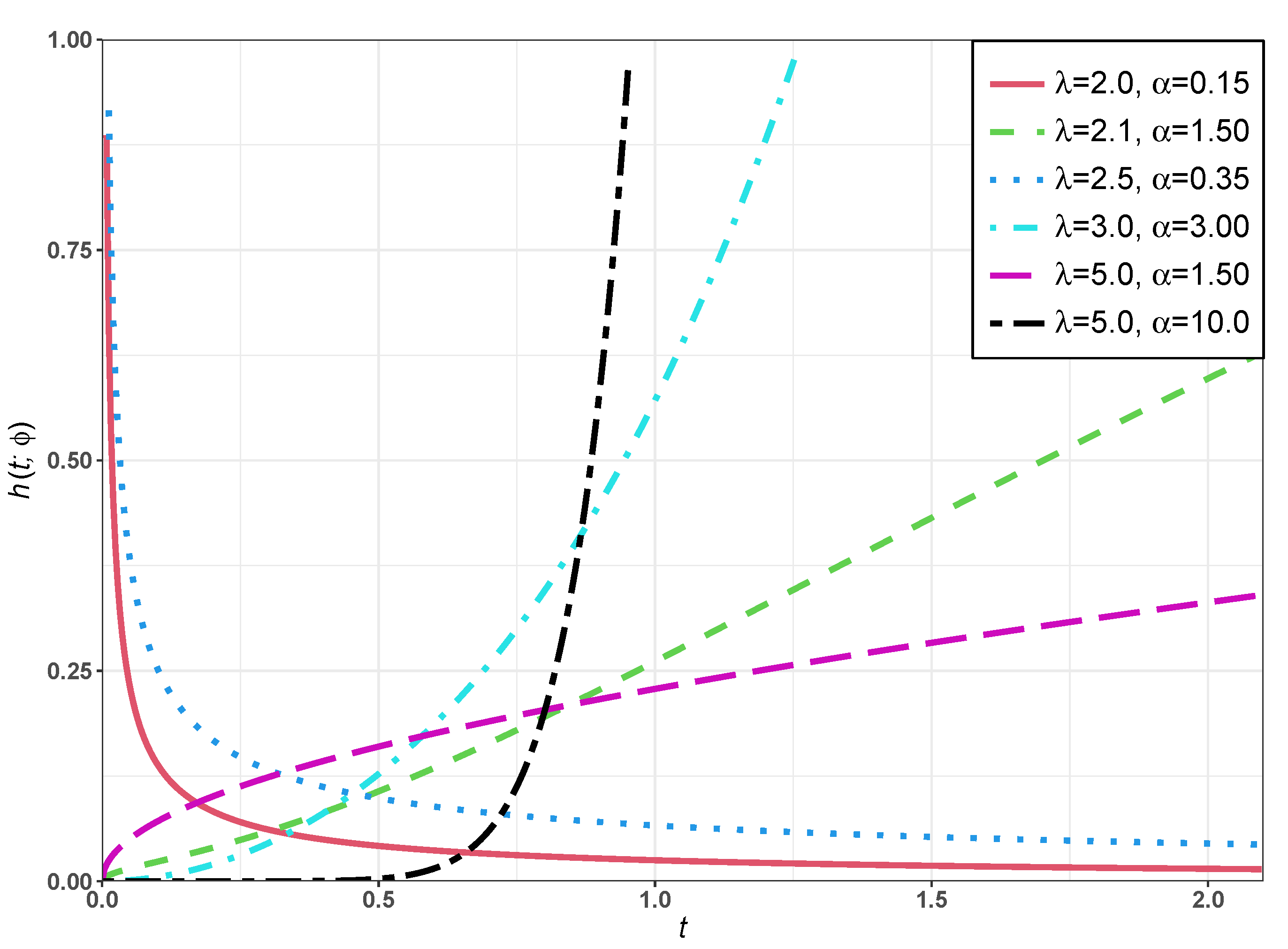
Figure 1 displays some possible shapes of HRF of the GRL for some selected values of λ and α . The shape of HRF can follow increasing, decreasing, reversed-J shaped, or J shaped hazard rates.

2.1. Shapes

The behavior of the PDF in (3) when t 0 and t are, respectively, given by
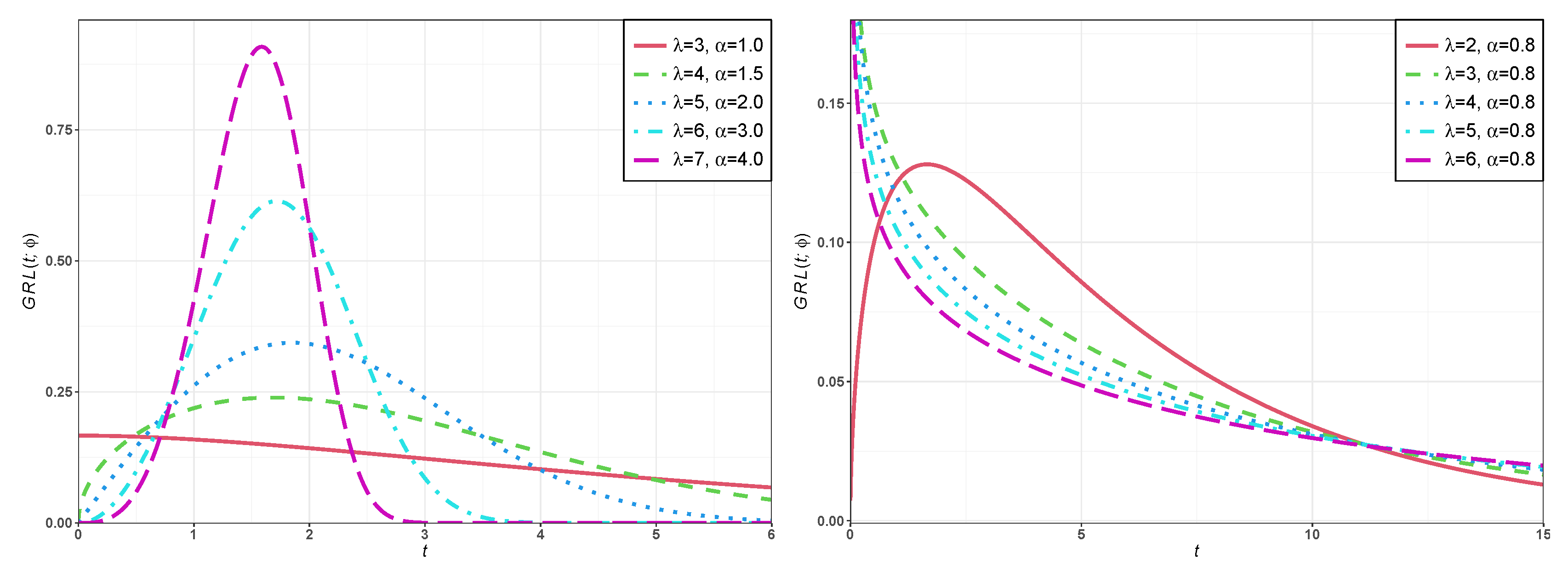
lim t 0 f ( t ; ϕ ) = , if α < 1 ( λ 2 ) λ ( λ 1 ) , if α = 1 0 , if α > 1 ,
lim t f ( t ; ϕ ) = 0 .
In Figure 2, we present the shapes of the PDF for different values of the parameters λ and α . The shape of PDF of the GRL model can be right-skewed or reversed-J shaped.

2.2. Quantile Function

The quantile function (QF) of the GRL distribution defined in (3), say, Q ( p ) wherein 0 < p < 1 , can be obtained by solving the equation F ( Q ( p ) ) = p in (4) for Q ( p ) in terms of p, and this implies
Q ( p ) = λ W 1 ( λ 1 ) ( p 1 ) e 1 λ + λ 1 1 / α ,
where W 1 ( · ) is the negative branch of the Lambert function.

2.3. Moments

Moments play an important role in statistical theory, so in this section we provide the r -th moment, the mean, and the variance for the GRL distribution.
Proposition 1.
For the random variable T that follows the GRL distribution, the r -th moment is given by
μ r = E [ T r ] = r λ r α α ( λ 1 ) λ + r α 1 Γ r α , f o r r N .
Proof. 
Note that the r-th moment for the random variable in (7) is given by
E [ T r ; α , λ ] = λ r α Γ r α + j , for j = 1 , 2 .
Since the GRL model can be expressed as a two-component mixture, as in (6), we have
μ r = E [ T r ] = 0 t r f ( t | α , λ ) d t = p E [ T r ; α , λ ] + ( 1 p ) E [ T r ; α + 1 , λ ] = λ 2 λ 1 λ r α Γ r α + 1 + 1 ( λ 1 ) λ r α Γ r α + 2 = r λ r α α ( λ 1 ) λ + r α 1 Γ r α ·
 □
Proposition 2.
The random variable T follows the GRL distribution; its mean and variance, respectively, are given by
μ = λ 1 α α ( λ 1 ) Γ 1 α λ + 1 α 1 a n d
σ 2 = λ 2 α α 2 ( λ 1 ) 2 2 α ( λ 1 ) Γ 2 α λ + 2 α 1 Γ 2 1 α λ + 1 α 1 2 .
Proof. 
From (9) and considering r = 1 , it follows that μ 1 = μ . The second result can be obtained by using σ 2 = E [ T 2 ] μ 2 and with some algebra the proof is completed. □
Proposition 3.
The r-th central moment for the GRL distribution is given by
M r = E [ T μ ] r = i = 0 r r i ( μ ) r i E [ T i ] = i = 0 r r i λ 1 α Γ α 1 α ( λ 1 ) λ + 1 α 1 r i i λ i α α ( λ 1 ) λ + i α 1 Γ i α .
Proof. 
The result follows directly from Proposition 1. □
The mean, variance, skewness, and kurtosis of the GRL distribution were computed numerically for different values of the parameters λ and α , using R software. Table 1 displays these numerical values. From Table 1 we can indicate that the skewness of the GRL distribution varies within the interval (−0.68158, 5.17333), whereas the skewness of the RL distribution can only range in the interval (1.41421, 1.85648) when the parameter λ takes values (2, 3.1, 4, 5.5). Furthermore, the spread of the kurtosis of the GRL distribution is much larger ranging, which is from 2.69447 to 52.6597, whereas the spread of the kurtosis of the RL distribution can only varies from 6.00 to 8.04 for the same values shown above for the parameter λ . The GRL model can also be left skewed or right skewed. Hence, the GRL distribution is a flexible distribution which can be used in modeling skewed data.

2.4. Order Statistics

Let T 1 , T 2 , T n be a random sample from (3) and T 1 : n T 2 : n T n : n denote the the corresponding order statistics. It is well known that the PDF and the CDF of the of r-th order statistics, say, T r : n and 1 r n , respectively, are given by
f r : n ( t ) = n ! ( r 1 ) ! ( n r ) ! [ F ( t ) ] r 1 [ 1 F ( t ) ] n r f ( t ) = n ! ( r 1 ) ! ( n r ) ! u = 0 n r ( 1 ) u n r u [ F ( t ) ] r 1 + u f ( t )
and
F r : n ( t ) = l = k n n l [ F ( t ) ] l [ 1 F ( t ) ] n l = l = k n u = 0 n r ( 1 ) u n l n r u [ F ( t ) ] l + u ,
for k = 1 , 2 , , n . It follows from (13) and (14) that the PDF and CDF of the r-th order statistic of the GRL reduce to
f r : n ( t ) = n ! ( λ 1 ) ( r 1 ) ! ( n r ) ! λ + t λ 2 e t λ u = 0 n r ( 1 ) u n r u × 1 1 λ 1 λ 1 + t α λ e t α λ r 1 + u
and
F r : n ( t ) = l = k n u = 0 n r ( 1 ) u n l n r u 1 1 λ 1 λ 1 + t α λ e t α λ l + u .

3. Estimation

In this section, we estimate of the GRL parameters λ and α using eight frequentist approaches. These methods are the weighted least-squares estimator (WLSE), ordinary least-squares estimator (OLSE), maximum likelihood estimator (MLE), maximum product of spacing estimator (MPSE), Cramér–von Mises estimator (CVME), Anderson–Darling estimator (ADE), right-tail Anderson–Darling estimator (RADE), and percentile based estimator (PCE).

3.1. Maximum Likelihood Estimators

In this sub-section we present the MLEs of the parameters λ and α of the GRL distribution.
Let t 1 , , t n be a sample from the GRL distribution given in (3). In this case, for ϕ = ( λ , α ) , the likelihood function from (3) is given by
L ( ϕ ; t ) = α n λ n + 1 ( λ 1 ) n i = 1 n t i α 1 i = 1 n λ 2 + t i α 2 λ exp 1 λ i = 1 n t i α .
The log-likelihood function l ( ϕ ; t ) = log L ( ϕ ; t ) is given by
l ( ϕ ; t ) = n log α ( n + 1 ) log ( λ ) n log ( λ 1 ) 1 λ i = 1 n t i α + ( α 1 ) i = 1 n log ( t i ) + i = 1 n log λ 2 + t i α 2 λ .
From the expressions λ l ( ϕ ; t ) = 0 , α l ( ϕ ; t ) = 0 , we get the likelihood equations
n + 1 λ n λ 1 + 1 λ 2 i = 1 n t i α + i = 1 n 2 ( λ 1 ) λ 2 + t i α 2 λ = 0
and
n α 1 λ i = 1 n t i α log ( t i ) + i = 1 n log ( t i ) + i = 1 n t i α log ( t i ) λ 2 + t i α 2 λ = 0 .
Under mild conditions [10] the ML estimates are asymptotically normal distributed with a bivariate normal distribution given by
( λ ^ , α ^ ) N 2 [ ( λ , α ) , H 1 ( λ , α ) ] for n   ,
where the elements of the observed Fisher information matrix H ( λ , α ) are given by
h 11 ( λ , α ) = n + 1 λ 2 n ( λ 1 ) 2 + 2 λ 3 i = 1 n t i α i = 1 n 2 ( t i α λ 2 + 2 λ 2 ) λ 2 + t i α 2 λ 2 ,
h 12 ( λ , α ) = h 21 ( α , λ ) = 1 λ 2 i = 1 n t i α log ( t i ) + i = 1 n 2 ( λ 1 ) t i α log ( t i ) λ 2 + t i α 2 λ 2 ,
h 22 ( λ , α ) = + n α 2 + 1 λ i = 1 n t i α log ( t i ) 2 i = 1 n λ ( λ 2 ) t i α log ( t i ) 2 λ 2 + t i α 2 λ 2 .
This can also be done by using different programs, namely, R (optim function) and SAS (PROC NLMIXED), or by solving the nonlinear likelihood equations obtained by differentiating .

3.2. Ordinary and Weighted Least-Squares Estimators

Let t ( 1 ) , t ( 2 ) , , t ( n ) be the order statistics of a sample of size n from F t ; λ , α in (4). Take the OLSE from [11]. λ ^ L S E and α ^ L S E can be obtained by minimizing
V λ , α = i = 1 n F t ( i ) | λ , α i n + 1 2 ,
with respect to λ and α . Or equivalently, the OLSEs follow by solving the non-linear equations
i = 1 n F t ( i ) | λ , α i n + 1 Δ s t ( i ) | λ , α = 0 , s = 1 , 2 ,
where
Δ 1 t ( i ) | λ , α = λ F t ( i ) | λ , α and Δ 2 t ( i ) | λ , α = α F t ( i ) | λ , α .
Note that the solution of Δ s for s = 1 , 2 can be obtained numerically.
The WLSEs [11] λ ^ W L S E and α ^ W L S E can be obtained by minimizing the following equation:
W λ , α = i = 1 n n + 1 2 n + 2 i n i + 1 F t ( i ) | λ , α i n + 1 2 .
Further, the WLSEs can also be derived by solving the non-linear equations:
i = 1 n n + 1 2 n + 2 i n i + 1 F t ( i ) | λ , α i n + 1 Δ s t ( i ) | λ , α = 0 , s = 1 , 2 ,
where Δ 1 · | λ , α and Δ 2 · | λ , α are provided in (17).

3.3. Maximum Product of Spacing Estimators

The maximum product of the spacings method [12,13,14], as an approximation of the Kullback–Leibler information measure, is a good alternative to the maximum likelihood method.
Let D i ( λ , α ) = F t ( i ) | λ , α F t ( i 1 ) | λ , α , for i = 1 , 2 , , n + 1 , be the uniform spacing of a random sample from the GRL distribution, where F t ( 0 ) | λ , α = 0 , F t ( n + 1 ) | λ , α = 1 and i = 1 n + 1 D i ( λ , α ) = 1 . The MPSE for λ ^ M P S E and α ^ M P S E can be obtained by maximizing the geometric mean of the spacing
G λ , α = i = 1 n + 1 D i ( λ , α ) 1 n + 1 ,
with respect to λ and α , or, equivalently, by maximizing the logarithm of the geometric mean of sample spacings
H λ , α = 1 n + 1 i = 1 n + 1 log D i ( λ , α ) .
The MPSE of the GRL parameters can be obtained by solving the nonlinear equations defined by
1 n + 1 i = 1 n + 1 1 D i ( λ , α ) Δ s ( t ( i ) | λ , α ) Δ s ( t ( i 1 ) | λ , α ) = 0 , s = 1 , 2 ,
where Δ 1 · | λ , α and Δ 2 · | λ , α are defined in (17).

3.4. The Cramér–von Mises Minimum Distance Estimators

The CVME, as a type of minimum distance estimator, has less bias than the other minimum distance estimators [15]. The CVMEs are obtained based on the difference between the estimates of the CDF and the empirical distribution function [16]. The CVMEs of the GRL parameters are obtained by minimizing
C ( λ , α ) = 1 12 n + i = 1 n F t ( i ) | λ , α 2 i 1 2 n 2 ,
with respect to λ and α . Further, the CVMEs follow by solving the non-linear equations:
i = 1 n F t ( i ) | λ , α 2 i 1 2 n Δ s t ( i ) | λ , α = 0 , s = 1 , 2 ,
where Δ 1 · | λ , α and Δ 2 · | λ , α are provided in (17).

3.5. The Anderson–Darling and Right-Tail Anderson–Darling Estimators

The Anderson–Darling statistic or Anderson–Darling estimator is another type of minimum distance estimator. The ADEs of the GRL parameters are obtained by minimizing
A ( λ , α ) = n 1 n i = 1 n 2 i 1 log F t ( i ) | λ , α + log S t ( i ) | λ , α ,
with respect to λ and α . These ADE can also be obtained by solving the non-linear equations
i = 1 n 2 i 1 Δ s t ( i ) | λ , α F t ( i ) | λ , α Δ j t ( n + 1 i ) | λ , α S t ( n + 1 i ) | λ , α = 0 , s = 1 , 2 .
The RADEs of the GRL parameters are obtained by minimizing
R ( λ , α ) = n 2 2 i = 1 n F t i : n | λ , α 1 n i = 1 n 2 i 1 log S t n + 1 i : n | λ , α ,
with respect to λ and α . The RADE can also be obtained by solving the non-linear equations
2 i = 1 n Δ s t i : n | λ , α + 1 n i = 1 n 2 i 1 Δ s t n + 1 i : n | λ , α S t n + 1 i : n | λ , α = 0 , s = 1 , 2 .
where Δ 1 · | λ , α and Δ 2 · | λ , α are defined in Equation (17).

3.6. Percentile Estimators

This method was originally suggested by [17,18]. Let u i = i / n + 1 be an unbiased estimator of F t ( i ) | λ , α . Then, the PCE of the parameters of GRL distribution are obtained by minimizing the following function
P ( λ , α ) = i = 1 n t ( i ) λ W 1 ( λ 1 ) ( u i 1 ) e 1 λ + λ 1 1 / α 2 ,
with respect to λ and α , where W 1 ( · ) is the negative branch of the Lambert function.

4. Simulation Analysis

A simulation study was conducted to explore and compare the behavior of the estimates with respect to their: average of absolute value of biases ( | B i a s ( ϕ ^ ) | ), | B i a s ( ϕ ^ ) | = 1 N i = 1 N | ϕ ^ ϕ | , average of mean square errors (MSEs), M S E s = 1 N i = 1 N ( ϕ ^ ϕ ) 2 , and average of mean relative errors (MREs), M R E s = 1 N i = 1 N | ϕ ^ ϕ | / ϕ .
We generated N = 5000 random samples T 1 , T 2 , , T N of sizes n = 30 , 50 , 80 , 100, and 200 from the GRL model by using Equation (8) while choosing λ = { 2.0 , 4.5 } and α = { 0.5 , 2.5 , 0.7 , 3.5 } ; we used R software (version 4.0.2) [19]. For each parameter combination and each sample, we estimated the GRL parameters λ and α using eight frequentist estimators including WLSE, OLSE, MLE, MPSE, CVME, ADE, RADE, and PCE. Then, the MSEs and MREs of the parameter estimates were computed. Simulated outcomes are listed in Table 2, Table 3, Table 4, Table 5, Table 6, Table 7, Table 8 and Table 9. Furthermore, these tables show the rank of each of the estimators among all the estimators in each row; the superscripts are the indicators, and the R a n k s is the partial sum of the ranks for each column in a certain sample size. Table 10 shows the partial and overall ranks of the estimators.
From Table 2, Table 3, Table 4, Table 5, Table 6, Table 7, Table 8 and Table 9, we can observe that:
  • All estimation methods show the property of consistency, i.e., the MSEs and MREs decrease as sample size increases, for all parameter combinations, except the weighted least-squares method.
  • The weighted least-squares method shows the property of consistency for all parameter combinations, except the combinations ϕ = ( λ = 3.1 , α = 0.7 ) T and ϕ = ( λ = 3.1 , α = 3.5 ) T , for the parameter λ .
From Table 10, and for the parameter combinations, we can conclude that the MPSE outperforms all the other estimators with an overall score of 62. Therefore, based on our study, we can confirm the superiority of MPSE and ADE for the GRL distribution.

5. Real Data Analysis

In this section, we illustrate the importance of the GRL distribution in modeling skewed data using two real datasets from the medicine and geology fields. The first dataset represents the survival times, in weeks, of 33 patients suffering from acute myelogeneous leukemia [20]. This dataset had already been analyzed by [21,22,23]. The second dataset was used to evaluate the risks associated with earthquakes occurring close to the central site of a nuclear power plant. This dataset refers to the distances, in miles, to the nuclear power plant of the most recent eight earthquakes of intensity larger than a given value [24] and it consists of 60 observations. It is noted that both datasets are unimodal based on the Hartigans’ dip test for the unimodality/multimodality test by using the function d i p . t e s t which is available within the R package diptest [25]. The null hypothesis: the data have a uni-modal distribution. The p-value (PV) of the first dataset was 0.8238, and 0.1507 was that of the second dataset; hence, we failed to reject the null hypothesis in the both cases at the 5 % significance level; thus, both datasets are unimodal.
The fits of the GRL distribution is compared with other competitive models which are given in Table 11, and their densities (for t > 0 ) are given by:
MOEx: f ( t ) = α λ exp ( λ t ) 1 1 α exp ( λ t ) 2 .
BEx: f ( t ) = λ B ( a , b ) exp ( b λ t ) 1 exp ( λ t ) a 1 .
EEx: f ( t ) = α λ exp ( λ t ) 1 exp ( λ t ) α 1 .
Ga: f ( t ) = b a Γ a t a 1 exp t / b .
GLi: f ( t ) = α λ 2 λ + 1 1 + t exp ( λ t ) 1 1 + λ + λ t λ + 1 exp ( λ t ) α 1 .
TTLi: f t = a 2 α + a ( 1 + α t ) exp ( a t ) 1 + λ 2 λ 1 α + a + α a t α + a exp ( a t ) .
PLx: f t = α β λ 1 + β t α 1 exp λ 1 + β t α 1 exp ( λ ) 1 .
LiGc: f t = 1 1 + a t a + 1 exp ( a t ) / 1 α 1 + a t a + 1 exp ( a t ) .
Li: f t = λ 2 λ + 1 1 + t exp ( λ t ) .
The parameters of the above densities are all positive real numbers except λ 1 for the TTLi distribution and α 0 , 1 for the LiGc distribution.
We considered some measures of goodness-of-fit, namely, minus maximized log-likelihood ( ^ ), Cramér–Von Mises ( W * ), Anderson–Darling ( A * ), and Kolmogorov–Smirnov (KS) statistics with bootstrapped (PV), to compare the fits of the GRL distribution with other competitive models. The results of these measures, for both datasets, are given in Table 12 and Table 13. We drew 999 , 999 bootstrap samples to obtain the KS bootstrapped PV.
The numerical values of ^ , W * , A * , KS, and bootstrapped PV, the MLEs, and their corresponding standard errors (SEs) (given in parentheses) of the fitted models are listed in Table 12 and Table 13, for both datasets, respectively. The figures in these tables show that the GRL distribution has the lowest values for all goodness-of-fit statistics among all fitted models.
Table 14 and Table 15 display the parameter estimates under various estimation methods and the goodness-of-fit statistics for both datasets, respectively. From Table 14 and Table 15, and based on the K S bootstrapped PV, we recommend using the MPSE to estimate the parameters of the GRL distribution for leukemia data, while the OLS method is recommended to estimate the GRL parameters for epicenter data.
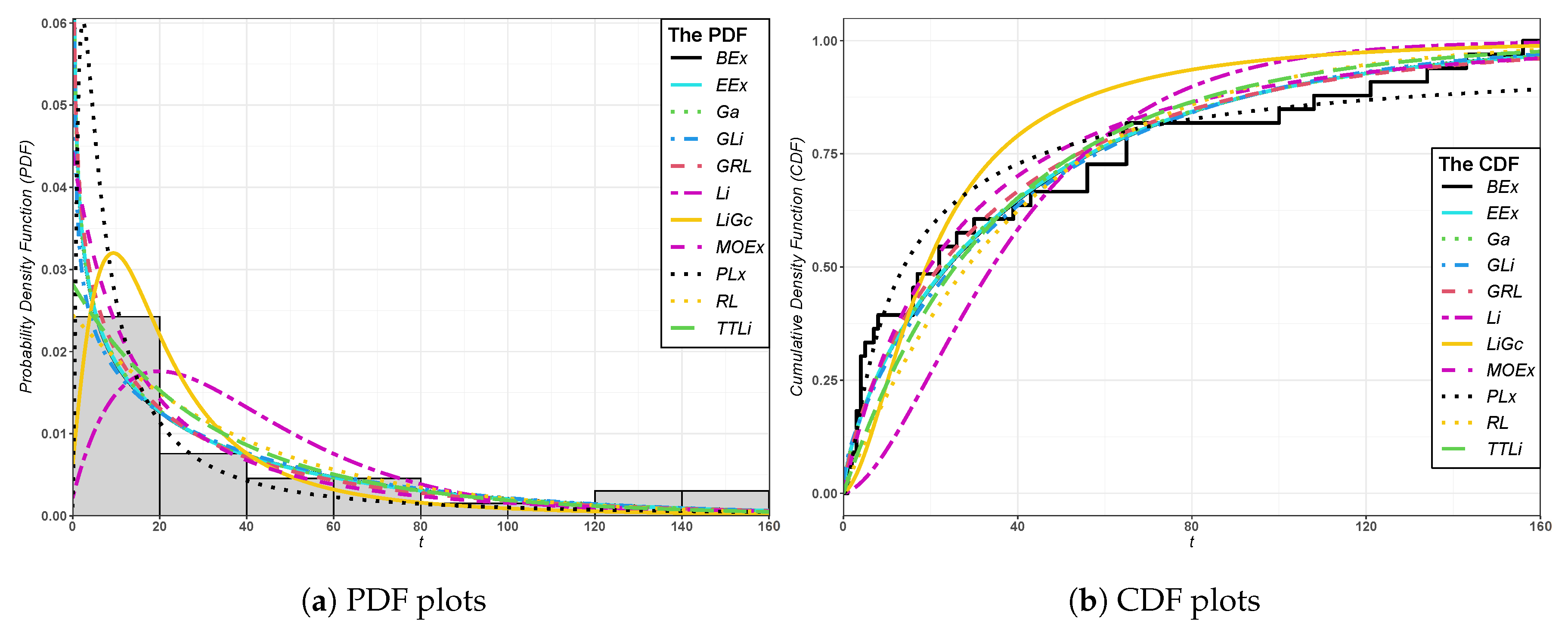
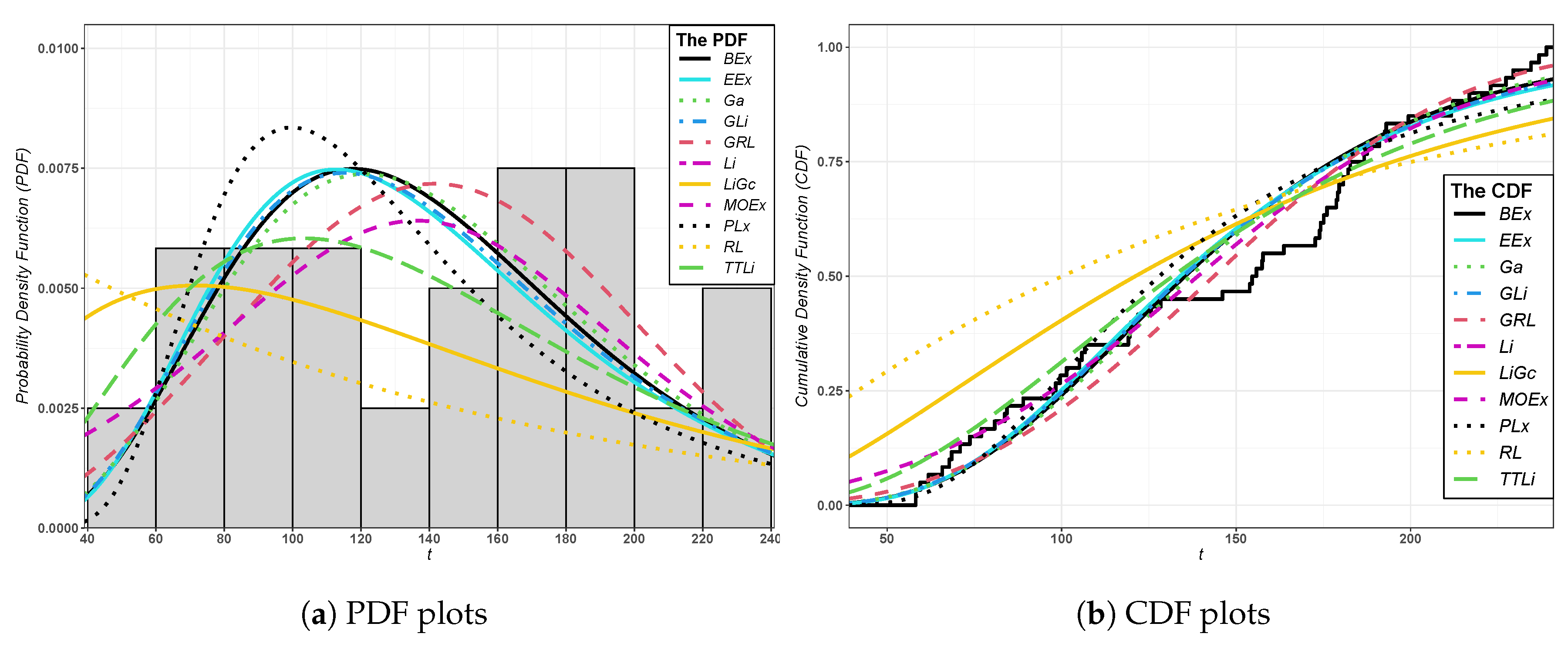
The histogram of the fitted GRL distribution and the other distributions are displayed in Figure 3 and Figure 4 for the two datasets, respectively. Figure 3 and Figure 4 show the plots of PDFs and CDFs of the fitted models for leukemia and epicenter data. The HRF plot of the GRL distribution and the TTT plot of leukemia data are displayed in Figure 5, whereas the HRF plot of the GRL distribution and the TTT plot of epicenter data are displayed in Figure 6. It is shown that the HRF is decreasing for leukemia data, whereas the HRF is increasing for epicenter data. Furthermore, the scaled TTT plot for the leukemia data is convex, which indicates a decreasing HRF, and it is concave for epicenter data, which indicates an increasing HRF. Thus, the GRL distribution is suitable for modeling leukemia and epicenter data.

6. Concluding Remarks

In this paper, we introduced a new two-parameter distribution called the generalized Ramos–Louzada (GRL) distribution. Further, the mathematical properties of the GRL model were studied in detail. The GRL parameters are estimated by eight estimation methods—namely, the weighted least-squares, ordinary least squares, maximum likelihood, maximum product of spacing, Cramér–von Mises, Anderson–Darling, right-tail Anderson–Darling, and percentile based estimators. The simulation study illustrated that the maximum product of the spacing method outperforms all other estimation methods. Therefore, based on our study, we can confirm the superiority of the maximum product of spacing method for the GRL distribution. Finally, the practical importance of GRL model was reported in two real applications. The goodness of fit for the proposed datasets showed that our model returned better fitting in comparison with other well-known distributions. Further, the two real data applications showed that the maximum product of the spacing estimator for the leukemia data and the least-square estimator for the epicenter data return the best estimates for the parameters of the GRL distribution.

Author Contributions

Conceptualization, H.A.-M.; methodology, A.Z.A.; software, H.A.-M.; validation, H.A.-M. and A.Z.A.; investigation, H.A.-M. and A.Z.A.; resources, H.A.-M. and A.Z.A.; writing—original draft preparation, H.A.-M. and A.Z.A.; writing—review and editing, H.A.-M., A.Z.A. and N.A.I.; supervision, A.Z.A.; project administration, A.Z.A.; funding acquisition, N.A.I. All authors have read and agreed to the revised version of the manuscript.

Funding

This research received no external funding.

Acknowledgments

The authors would like to thank the editor and two reviewers for their constructive comments and suggestions which greatly improved the final version of the manuscript.

Conflicts of Interest

The authors declare no conflict of interest.

References

  1. Ramos, P.L.; Louzada, F. A distribution for instantaneous failures. Stats 2019, 2, 247–258. [Google Scholar] [CrossRef] [Green Version]
  2. Weibull, W. A statistical distribution function of wide applicability. J. Appl. Mech. 1951, 18, 293–297. [Google Scholar]
  3. Gupta, R.D.; Kundu, D. Exponentiated exponential family: An alternative to gamma and Weibull distributions. J. Math. Methods Biosci. 2001, 43, 117–130. [Google Scholar] [CrossRef]
  4. Ghitany, M.; Al-Mutairi, D.; Balakrishnan, N.; Al-Enezi, L. Power Lindley distribution and associated inference. Comput. Stat. Data Anal. 2013, 64, 20–33. [Google Scholar] [CrossRef]
  5. Nadarajah, S.; Bakouch, H.S.; Tahmasbi, R. A generalized Lindley distribution. Sankhya B 2011, 73, 331–359. [Google Scholar] [CrossRef]
  6. Stacy, E.W. A generalization of the gamma distribution. Ann. Math. Stat. 1962, 33, 1187–1192. [Google Scholar] [CrossRef]
  7. Nassar, M.; Afify, A.Z.; Shakhatreh, M. Estimation methods of alpha power exponential distribution with applications to engineering and medical Data. Pak. J. Stat. Oper. Res. 2020, 16, 149–166. [Google Scholar] [CrossRef]
  8. Afify, A.Z.; Mohamed, O.A. A new three-parameter exponential distribution with variable shapes for the hazard rate: Estimation and applications. Mathematics 2020, 8, 135. [Google Scholar] [CrossRef] [Green Version]
  9. Afify, A.Z.; Nassar, M.; Cordeiro, G.M.; Kumar, D. The Weibull Marshall–Olkin Lindley distribution: Properties and estimation. J. Taibah Univ. Sci. 2020, 14, 192–204. [Google Scholar] [CrossRef]
  10. Migon, H.S.; Gamerman, D.; Louzada, F. Statistical Inference: An Integrated Approach; CRC Press: New York, NY, USA, 2014. [Google Scholar]
  11. Swain, J.J.; Venkatraman, S.; Wilson, J.R. Least-squares estimation of distribution functions in johnson’s translation system. J. Stat. Comput. Simul. 1988, 29, 271–297. [Google Scholar] [CrossRef]
  12. Cheng, R.; Amin, N. Maximum Product of Spacings Estimation with Application to the Lognormal Distribution; Mathematical Report 79-1; University of Wales: Cardiff, UK, 1979. [Google Scholar]
  13. Cheng, R.; Amin, N. Estimating parameters in continuous univariate distributions with a shifted origin. J. R. Stat. Soc. Ser. B Methodol. 1983, 45, 394–403. [Google Scholar] [CrossRef]
  14. Ranneby, B. The maximum spacing method. An estimation method related to the maximum likelihood method. Scand. J. Stat. 1984, 11, 93–112. [Google Scholar]
  15. Macdonald, P. Comment on “an estimation procedure for mixtures of distributions” by Choi and Bulgren. J. R. Stat. Soc. Ser. B Methodol. 1971, 33, 326–329. [Google Scholar]
  16. Luceño, A. Fitting the generalized pareto distribution to data using maximum goodness-of-fit estimators. Comput. Stat. Data Anal. 2006, 51, 904–917. [Google Scholar] [CrossRef]
  17. Kao, J. Computer methods for estimating Weibull parameters in reliability studies. IRE Reliab. Qual. Control 1958, 13, 15–22. [Google Scholar] [CrossRef]
  18. Kao, J. A graphical estimation of mixed Weibull parameters in life testing electron tube. Technometrics 1959, 1, 389–407. [Google Scholar] [CrossRef]
  19. R Core Team. R: A Language and Environment for Statistical Computing; R Foundation for Statistical Computing: Vienna, Austria, 2020; Available online: https://www.R-project.org (accessed on 22 June 2020).
  20. Feigl, P.; Zelen, M. Estimation of exponential probabilities with concomitant information. Biometrics 1965, 21, 826–838. [Google Scholar] [CrossRef]
  21. Abouelmagd, T.H.M.; Hamed, M.S.; Afify, A.Z.; Al-Mofleh, H.; Iqbal, Z. The Burr X Fréchet distribution with its properties and applications. J. Appl. Probab. Stat. 2018, 13, 23–51. [Google Scholar]
  22. Nassar, M.; Afify, A.Z.; Dey, S.; Kumar, D. A new extension of Weibull distribution: Properties and different methods of estimation. J. Comput. Appl. Math. 2018, 336, 439–457. [Google Scholar] [CrossRef]
  23. Sen, S.; Afify, A.Z.; Al-Mofleh, H.; Ahsanullah, M. The quasi Xgamma-geometric distribution with application in medicine. Filomat 2019, 33, 5291–5330. [Google Scholar] [CrossRef] [Green Version]
  24. Castillo, E. Extreme Value Theory in Engineering; Elsevier: Amsterdam, The Netherlands, 2012. [Google Scholar]
  25. Maechler, M. Diptest: Hartigan’s Dip Test Statistic for Unimodality—Corrected: R Package Version 0.75-7. 2016. Available online: https://CRAN.R-project.org/ (accessed on 5 December 2016).
  26. Marshall, A.W.; Olkin, I. A new method for adding a parameter to a family of distributions with application to the exponential and Weibull families. Biometrika 1997, 84, 641–652. [Google Scholar] [CrossRef]
  27. Jones, M.C. Families of distributions arising from distributions of order statistics. Test 2004, 13, 1–43. [Google Scholar] [CrossRef]
  28. Beyer, W.H. CRC Standard Mathematical Tables, 30th ed.; CRC: Boca Raton, FL, USA, 1996. [Google Scholar]
  29. Kemaloglu, S.A.; Yilmaz, M. Transmuted two-parameter Lindley distribution. Commun. Stat. Theory Methods 2017, 46, 11866–11879. [Google Scholar] [CrossRef]
  30. Al-Zahrani, B.; Sagor, H. The Poisson-lomax distribution. Rev. Colomb. Estad. 2014, 37, 225–245. [Google Scholar] [CrossRef]
  31. Zakerzadeh, H.; Mahmoudi, E. A new two parameter lifetime distribution: Model and properties. arXiv 2012, arXiv:1204.4248. [Google Scholar]
  32. Lindley, D.V. Fiducial distributions and Bayes theorem. J. R. Stat. Soc. 1958, 20, 102–107. [Google Scholar] [CrossRef]
Figure 1. Hazard rat function shapes for the generalized Ramos–Louzada distribution considering different values of λ and α .
Mathematics 08 01578 g001
Figure 2. PDF shapes for the GRL distribution considering different values of λ and α .
Mathematics 08 01578 g002
Figure 3. Fitted densities and distribution functions of the competing models for leukemia data.
Mathematics 08 01578 g003
Figure 4. Fitted densities and distribution functions of the competing models for epicenter data.
Mathematics 08 01578 g004
Figure 5. The hazard rate function (HRF) plot of the GRL distribution and TTT plot for leukemia data.
Mathematics 08 01578 g005
Figure 6. The HRF plot of the GRL distribution and TTT plot for epicenter data.
Mathematics 08 01578 g006
Table 1. Mean, variance, skewness, and kurtosis of the GRL distribution for different values of the parameters λ and α .
ϕ MeanVarianceSkewnessKurtosis
( λ = 2.0 , α = 0.5 ) 24.001344.004.3037.41
( λ = 2.0 , α = 0.7 ) 8.2772.442.3912.65
( λ = 2.0 , α = 2.5 ) 1.640.230.202.89
( λ = 2.0 , α = 3.5 ) 1.410.09−0.042.88
( λ = 3.1 , α = 0.5 ) 37.525030.155.1752.66
( λ = 3.1 , α = 0.7 ) 10.71186.232.8516.24
( λ = 3.1 , α = 2.5 ) 1.660.420.182.73
( λ = 3.1 , α = 3.1 ) 1.490.23−0.032.71
( λ = 4.0 , α = 1.5 ) 2.783.190.923.89
( λ = 4.0 , α = 3.5 ) 1.460.20−0.072.71
( λ = 4.0 , α = 5.0 ) 1.290.08−0.352.95
( λ = 4.0 , α = 10 ) 1.130.02−0.733.74
( λ = 5.5 , α = 3.5 ) 1.560.23−0.032.69
( λ = 5.5 , α = 5.0 ) 1.350.09−0.302.90
( λ = 5.5 , α = 5.5 ) 1.310.07−0.362.99
( λ = 5.5 , α = 10 ) 1.150.02−0.683.64
Table 2. Simulation results for ϕ = ( λ = 2.0 , α = 0.5 ) .
nEst.Est. Par.WLSEOLSEMLEMPSECVMEADERADEPCE
| B I A S | λ ^ 0.21560 { 4 } 0.25992 { 7 } 0.19097 { 2 } 0.24975 { 6 } 0.19471 { 3 } 0.18910 { 1 } 0.23949 { 5 } 0.60664 { 8 }
α ^ 0.04161 { 6 } 0.04378 { 8 } 0.03703 { 2 } 0.03455 { 1 } 0.04313 { 7 } 0.03896 { 4 } 0.03856 { 3 } 0.03931 { 5 }
M S E λ ^ 0.18356 { 3 } 0.23965 { 5 } 0.36520 { 7 } 0.27292 { 6 } 0.17386 { 2 } 0.16253 { 1 } 0.22387 { 4 } 2.80485 { 8 }
30 α ^ 0.00315 { 5 } 0.00347 { 7 } 0.00283 { 4 } 0.00210 { 1 } 0.00337 { 6 } 0.00262 { 3 } 0.00259 { 2 } 0.00516 { 8 }
M R E λ ^ 0.10780 { 4 } 0.12996 { 7 } 0.09549 { 2 } 0.12488 { 6 } 0.09736 { 3 } 0.09455 { 1 } 0.11975 { 5 } 0.30332 { 8 }
α ^ 0.08322 { 6 } 0.08755 { 8 } 0.07406 { 2 } 0.06909 { 1 } 0.08626 { 7 } 0.07791 { 4 } 0.07713 { 3 } 0.07861 { 5 }
R a n k s 28 { 5.5 } 42 { 7.5 } 19 { 2 } 21 { 3 } 28 { 5.5 } 14 { 1 } 22 { 4 } 42 { 7.5 }
| B I A S | λ ^ 0.13639 { 3 } 0.18362 { 6 } 0.12166 { 1 } 0.15871 { 5 } 0.14529 { 4 } 0.12558 { 2 } 0.1852 { 7 } 0.45425 { 8 }
α ^ 0.02936 { 5 } 0.03369 { 8 } 0.02734 { 2 } 0.02600 { 1 } 0.03270 { 7 } 0.02913 { 4 } 0.02955 { 6 } 0.02903 { 3 }
M S E λ ^ 0.09622 { 2 } 0.14769 { 4 } 0.19069 { 7 } 0.14789 { 5 } 0.11450 { 3 } 0.08491 { 1 } 0.15437 { 6 } 0.67882 { 8 }
50 α ^ 0.00150 { 3 } 0.00197 { 8 } 0.00156 { 4.5 } 0.00123 { 1 } 0.00186 { 6 } 0.00144 { 2 } 0.00156 { 4.5 } 0.00187 { 7 }
M R E λ ^ 0.06819 { 3 } 0.09181 { 6 } 0.06083 { 1 } 0.07936 { 5 } 0.07264 { 4 } 0.06279 { 2 } 0.09260 { 7 } 0.22712 { 8 }
α ^ 0.05873 { 5 } 0.06739 { 8 } 0.05469 { 2 } 0.05200 { 1 } 0.06540 { 7 } 0.05826 { 4 } 0.05910 { 6 } 0.05806 { 3 }
R a n k s 21 { 4 } 40 { 8 } 17.5 { 2 } 18 { 3 } 31 { 5 } 15 { 1 } 36.5 { 6 } 37 { 7 }
| B I A S | λ ^ 0.08834 { 2 } 0.12514 { 6 } 0.05967 { 1 } 0.09455 { 4 } 0.10202 { 5 } 0.08968 { 3 } 0.12941 { 7 } 0.42545 { 8 }
α ^ 0.02248 { 4 } 0.02583 { 8 } 0.01925 { 2 } 0.01906 { 1 } 0.02481 { 7 } 0.02247 { 3 } 0.02265 { 5 } 0.02466 { 6 }
M S E λ ^ 0.04546 { 2 } 0.07616 { 6 } 0.06131 { 5 } 0.05756 { 3 } 0.05795 { 4 } 0.04391 { 1 } 0.08631 { 7 } 0.66542 { 8 }
80 α ^ 0.00087 { 3.5 } 0.00114 { 7 } 0.00072 { 2 } 0.00064 { 1 } 0.00108 { 6 } 0.00087 { 3.5 } 0.00091 { 5 } 0.00140 { 8 }
M R E λ ^ 0.04417 { 2 } 0.06257 { 6 } 0.02983 { 1 } 0.04728 { 4 } 0.05101 { 5 } 0.04484 { 3 } 0.06471 { 7 } 0.21272 { 8 }
α ^ 0.04496 { 4 } 0.05165 { 8 } 0.03849 { 2 } 0.03812 { 1 } 0.04962 { 7 } 0.04494 { 3 } 0.04529 { 5 } 0.04932 { 6 }
R a n k s 17.5 { 4 } 41 { 7 } 13 { 1 } 14 { 2 } 34 { 5 } 16.5 { 3 } 36 { 6 } 44 { 8 }
| B I A S | λ ^ 0.06011 { 3 } 0.08382 { 6 } 0.03817 { 1 } 0.05747 { 2 } 0.07447 { 5 } 0.06168 { 4 } 0.09059 { 7 } 0.36554 { 8 }
α ^ 0.01795 { 5 } 0.02018 { 6 } 0.01511 { 2 } 0.01504 { 1 } 0.02037 { 7 } 0.01791 { 4 } 0.01785 { 3 } 0.02127 { 8 }
M S E λ ^ 0.01744 { 2 } 0.03412 { 6 } 0.02904 { 4 } 0.01501 { 1 } 0.03090 { 5 } 0.01893 { 3 } 0.04248 { 7 } 0.38789 { 8 }
120 α ^ 0.00053 { 3.5 } 0.00068 { 6 } 0.00043 { 2 } 0.00037 { 1 } 0.00070 { 7 } 0.00053 { 3.5 } 0.00055 { 5 } 0.00095 { 8 }
M R E λ ^ 0.03005 { 3 } 0.04191 { 6 } 0.01909 { 1 } 0.02874 { 2 } 0.03724 { 5 } 0.03084 { 4 } 0.04530 { 7 } 0.18277 { 8 }
α ^ 0.03590 { 5 } 0.04036 { 6 } 0.03022 { 2 } 0.03008 { 1 } 0.04074 { 7 } 0.03582 { 4 } 0.03570 { 3 } 0.04253 { 8 }
R a n k s 21.5 { 3 } 36 { 6.5 } 12 { 2 } 8 { 1 } 36 { 6.5 } 22.5 { 4 } 32 { 5 } 48 { 8 }
| B I A S | λ ^ 0.04146 { 4 } 0.05483 { 6 } 0.02171 { 1 } 0.03768 { 2 } 0.04827 { 5 } 0.04074 { 3 } 0.06524 { 7 } 0.29846 { 8 }
α ^ 0.01373 { 4 } 0.01528 { 7 } 0.01158 { 2 } 0.01126 { 1 } 0.01502 { 6 } 0.01344 { 3 } 0.01374 { 5 } 0.01693 { 8 }
M S E λ ^ 0.00755 { 4 } 0.01424 { 6 } 0.00364 { 1 } 0.00503 { 2 } 0.00929 { 5 } 0.00656 { 3 } 0.01827 { 7 } 0.25762 { 8 }
200 α ^ 0.00030 { 4 } 0.00039 { 7 } 0.00022 { 2 } 0.00021 { 1 } 0.00036 { 6 } 0.00029 { 3 } 0.00031 { 5 } 0.00062 { 8 }
M R E λ ^ 0.02073 { 4 } 0.02742 { 6 } 0.01086 { 1 } 0.01884 { 2 } 0.02413 { 5 } 0.02037 { 3 } 0.03262 { 7 } 0.14923 { 8 }
α ^ 0.02745 { 4 } 0.03056 { 7 } 0.02316 { 2 } 0.02252 { 1 } 0.03004 { 6 } 0.02689 { 3 } 0.02748 { 5 } 0.03385 { 8 }
R a n k s 24 { 4 } 39 { 7 } 9 { 1.5 } 9 { 1.5 } 33 { 5 } 18 { 3 } 36 { 6 } 48 { 8 }
Table 3. Simulation results for ϕ = ( λ = 2.0 , α = 2.5 ) .
nEst.Est. Par.WLSEOLSEMLEMPSECVMEADERADEPCE
| B I A S | λ ^ 0.21244 { 4 } 0.26189 { 8 } 0.19438 { 1 } 0.25088 { 7 } 0.19742 { 3 } 0.19522 { 2 } 0.24708 { 6 } 0.24484 { 5 }
α ^ 0.19894 { 6 } 0.22582 { 8 } 0.18894 { 3 } 0.16969 { 1 } 0.21786 { 7 } 0.19693 { 5 } 0.19001 { 4 } 0.18423 { 2 }
M S E λ ^ 0.19082 { 3 } 0.24426 { 6 } 0.37099 { 8 } 0.27879 { 7 } 0.17947 { 2 } 0.17346 { 1 } 0.23687 { 5 } 0.22556 { 4 }
30 α ^ 0.07158 { 5 } 0.09018 { 8 } 0.07436 { 6 } 0.05047 { 1 } 0.08317 { 7 } 0.06861 { 4 } 0.06401 { 3 } 0.05827 { 2 }
M R E λ ^ 0.10622 { 4 } 0.13095 { 8 } 0.09719 { 1 } 0.12544 { 7 } 0.09871 { 3 } 0.09761 { 2 } 0.12354 { 6 } 0.12242 { 5 }
α ^ 0.07958 { 6 } 0.09033 { 8 } 0.07558 { 3 } 0.06788 { 1 } 0.08715 { 7 } 0.07877 { 5 } 0.07600 { 4 } 0.07369 { 2 }
R a n k s 28 { 5.5 } 46 { 8 } 22 { 3 } 24 { 4 } 29 { 7 } 19 { 1 } 28 { 5.5 } 20 { 2 }
| B I A S | λ ^ 0.15218 { 4 } 0.19041 { 8 } 0.12832 { 1 } 0.16578 { 5 } 0.14117 { 3 } 0.13719 { 2 } 0.17754 { 7 } 0.16591 { 6 }
α ^ 0.15254 { 6 } 0.16622 { 8 } 0.13759 { 3 } 0.13128 { 1 } 0.16422 { 7 } 0.14949 { 5 } 0.14755 { 4 } 0.13745 { 2 }
M S E λ ^ 0.12789 { 3 } 0.15222 { 6 } 0.22581 { 8 } 0.15456 { 7 } 0.10804 { 2 } 0.10193 { 1 } 0.14774 { 5 } 0.13513 { 4 }
50 α ^ 0.04130 { 5 } 0.04890 { 8 } 0.04144 { 6 } 0.03102 { 1 } 0.04880 { 7 } 0.03916 { 4 } 0.03824 { 3 } 0.03382 { 2 }
M R E λ ^ 0.07609 { 4 } 0.09520 { 8 } 0.06416 { 1 } 0.08289 { 5 } 0.07058 { 3 } 0.06859 { 2 } 0.08877 { 7 } 0.08296 { 6 }
α ^ 0.06102 { 6 } 0.06649 { 8 } 0.05504 { 3 } 0.05251 { 1 } 0.06569 { 7 } 0.05980 { 5 } 0.05902 { 4 } 0.05498 { 2 }
R a n k s 28 { 5 } 46 { 8 } 22 { 3.5 } 20 { 2 } 29 { 6 } 19 { 1 } 30 { 7 } 22 { 3.5 }
| B I A S | λ ^ 0.09792 { 5 } 0.11640 { 7 } 0.06223 { 1 } 0.09687 { 4 } 0.09837 { 6 } 0.08741 { 2 } 0.12992 { 8 } 0.09557 { 3 }
α ^ 0.11506 { 6 } 0.12703 { 8 } 0.09758 { 2 } 0.09640 { 1 } 0.12599 { 7 } 0.11229 { 4 } 0.11275 { 5 } 0.10036 { 3 }
M S E λ ^ 0.06450 { 5 } 0.06699 { 6 } 0.07769 { 7 } 0.06419 { 4 } 0.05569 { 3 } 0.04415 { 1 } 0.08704 { 8 } 0.04739 { 2 }
80 α ^ 0.02399 { 6 } 0.02743 { 8 } 0.01923 { 3 } 0.01682 { 1 } 0.02688 { 7 } 0.02139 { 4 } 0.02313 { 5 } 0.01729 { 2 }
M R E λ ^ 0.04896 { 5 } 0.05820 { 7 } 0.03111 { 1 } 0.04843 { 4 } 0.04919 { 6 } 0.04370 { 2 } 0.06496 { 8 } 0.04778 { 3 }
α ^ 0.04602 { 6 } 0.05081 { 8 } 0.03903 { 2 } 0.03856 { 1 } 0.05039 { 7 } 0.04492 { 4 } 0.04510 { 5 } 0.04014 { 3 }
R a n k s 33 { 5 } 44 { 8 } 16 { 2.5 } 15 { 1 } 36 { 6 } 17 { 4 } 39 { 7 } 16 { 2.5 }
| B I A S | λ ^ 0.06067 { 2 } 0.08408 { 7 } 0.04208 { 1 } 0.06183 { 3 } 0.06947 { 6 } 0.06212 { 4 } 0.09096 { 8 } 0.06412 { 5 }
α ^ 0.08937 { 5 } 0.10170 { 8 } 0.07782 { 2 } 0.07594 { 1 } 0.09938 { 7 } 0.08778 { 4 } 0.08961 { 6 } 0.08093 { 3 }
M S E λ ^ 0.02061 { 1 } 0.03392 { 6 } 0.03763 { 7 } 0.02264 { 3 } 0.02543 { 5 } 0.02114 { 2 } 0.04016 { 8 } 0.02293 { 4 }
120 α ^ 0.01348 { 5 } 0.01715 { 8 } 0.01167 { 3 } 0.01002 { 1 } 0.01616 { 7 } 0.01292 { 4 } 0.01362 { 6 } 0.01103 { 2 }
M R E λ ^ 0.03033 { 2 } 0.04204 { 7 } 0.02104 { 1 } 0.03091 { 3 } 0.03474 { 6 } 0.03106 { 4 } 0.04548 { 8 } 0.03206 { 5 }
α ^ 0.03575 { 5 } 0.04068 { 8 } 0.03113 { 2 } 0.03037 { 1 } 0.03975 { 7 } 0.03511 { 4 } 0.03584 { 6 } 0.03237 { 3 }
R a n k s 20 { 3 } 44 { 8 } 16 { 2 } 12 { 1 } 38 { 6 } 22 { 4.5 } 42 { 7 } 22 { 4.5 }
| B I A S | λ ^ 0.03782 { 2 } 0.05703 { 7 } 0.02118 { 1 } 0.03827 { 3 } 0.04951 { 6 } 0.03908 { 4 } 0.06286 { 8 } 0.04085 { 5 }
α ^ 0.06707 { 5 } 0.07506 { 7 } 0.05763 { 2 } 0.05660 { 1 } 0.07580 { 8 } 0.06811 { 6 } 0.0667 { 4 } 0.05915 { 3 }
M S E λ ^ 0.00618 { 3 } 0.01328 { 7 } 0.00639 { 4 } 0.00498 { 1 } 0.01080 { 6 } 0.00681 { 5 } 0.01851 { 8 } 0.00576 { 2 }
200 α ^ 0.00738 { 4 } 0.00911 { 7 } 0.00559 { 3 } 0.00520 { 1 } 0.00931 { 8 } 0.00739 { 5 } 0.00745 { 6 } 0.00554 { 2 }
M R E λ ^ 0.01891 { 2 } 0.02852 { 7 } 0.01059 { 1 } 0.01913 { 3 } 0.02476 { 6 } 0.01954 { 4 } 0.03143 { 8 } 0.02043 { 5 }
α ^ 0.02683 { 5 } 0.03002 { 7 } 0.02305 { 2 } 0.02264 { 1 } 0.03032 { 8 } 0.02724 { 6 } 0.02668 { 4 } 0.02366 { 3 }
R a n k s 21 { 4 } 42 { 7.5 } 13 { 2 } 10 { 1 } 42 { 7.5 } 30 { 5 } 38 { 6 } 20 { 3 }
Table 4. Simulation results for ϕ = ( λ = 2.0 , α = 0.7 ) .
nEst.Est. Par.WLSEOLSEMLEMPSECVMEADERADEPCE
| B I A S | λ ^ 0.21445 { 4 } 0.25938 { 7 } 0.19354 { 2 } 0.24781 { 6 } 0.19844 { 3 } 0.18907 { 1 } 0.24632 { 5 } 0.34260 { 8 }
α ^ 0.05581 { 3 } 0.08771 { 8 } 0.07506 { 5 } 0.04727 { 1 } 0.08616 { 7 } 0.07770 { 6 } 0.05562 { 2 } 0.07092 { 4 }
M S E λ ^ 0.18452 { 3 } 0.23540 { 4 } 0.36081 { 7 } 0.27295 { 6 } 0.18169 { 2 } 0.16400 { 1 } 0.23850 { 5 } 0.37356 { 8 }
30 α ^ 0.00563 { 3 } 0.01365 { 8 } 0.01143 { 6 } 0.00388 { 1 } 0.01301 { 7 } 0.01055 { 5 } 0.00535 { 2 } 0.00939 { 4 }
M R E λ ^ 0.10723 { 4 } 0.12969 { 7 } 0.09677 { 2 } 0.12391 { 6 } 0.09922 { 3 } 0.09454 { 1 } 0.12316 { 5 } 0.17130 { 8 }
α ^ 0.07972 { 6 } 0.08771 { 8 } 0.07506 { 3 } 0.06753 { 1 } 0.08616 { 7 } 0.07770 { 4 } 0.07946 { 5 } 0.07092 { 2 }
R a n k s 23 { 3 } 42 { 8 } 25 { 5 } 21 { 2 } 29 { 6 } 18 { 1 } 24 { 4 } 34 { 7 }
| B I A S | λ ^ 0.13755 { 3 } 0.18644 { 6 } 0.12791 { 1 } 0.15661 { 5 } 0.14790 { 4 } 0.13583 { 2 } 0.18659 { 7 } 0.26307 { 8 }
α ^ 0.04117 { 2 } 0.06716 { 8 } 0.05516 { 5 } 0.03626 { 1 } 0.06619 { 7 } 0.05860 { 6 } 0.04165 { 3 } 0.05464 { 4 }
M S E λ ^ 0.09565 { 1 } 0.14451 { 4 } 0.21621 { 7 } 0.15337 { 5 } 0.11738 { 3 } 0.09943 { 2 } 0.15757 { 6 } 0.22931 { 8 }
50 α ^ 0.00302 { 2 } 0.00780 { 8 } 0.00654 { 6 } 0.00237 { 1 } 0.00770 { 7 } 0.00598 { 5 } 0.00308 { 3 } 0.00518 { 4 }
M R E λ ^ 0.06877 { 3 } 0.09322 { 6 } 0.06395 { 1 } 0.07831 { 5 } 0.07395 { 4 } 0.06792 { 2 } 0.09330 { 7 } 0.13153 { 8 }
α ^ 0.05882 { 5 } 0.06716 { 8 } 0.05516 { 3 } 0.05180 { 1 } 0.06619 { 7 } 0.05860 { 4 } 0.05950 { 6 } 0.05464 { 2 }
R a n k s 16 { 1 } 40 { 8 } 23 { 4 } 18 { 2 } 32 { 5.5 } 21 { 3 } 32 { 5.5 } 34 { 7 }
| B I A S | λ ^ 0.08945 { 3 } 0.12477 { 6 } 0.06659 { 1 } 0.09352 { 4 } 0.09986 { 5 } 0.08396 { 2 } 0.12731 { 7 } 0.19421 { 8 }
α ^ 0.03115 { 3 } 0.05100 { 8 } 0.03940 { 4 } 0.02693 { 1 } 0.05047 { 7 } 0.04567 { 6 } 0.03092 { 2 } 0.04264 { 5 }
M S E λ ^ 0.04583 { 2 } 0.07469 { 5 } 0.07839 { 7 } 0.05851 { 4 } 0.05740 { 3 } 0.03994 { 1 } 0.07827 { 6 } 0.14794 { 8 }
80 α ^ 0.00168 { 2.5 } 0.00447 { 8 } 0.00311 { 4 } 0.00129 { 1 } 0.00428 { 7 } 0.00354 { 6 } 0.00168 { 2.5 } 0.00314 { 5 }
M R E λ ^ 0.04473 { 3 } 0.06239 { 6 } 0.03329 { 1 } 0.04676 { 4 } 0.04993 { 5 } 0.04198 { 2 } 0.06366 { 7 } 0.09710 { 8 }
α ^ 0.04450 { 5 } 0.05100 { 8 } 0.03940 { 2 } 0.03848 { 1 } 0.05047 { 7 } 0.04567 { 6 } 0.04417 { 4 } 0.04264 { 3 }
R a n k s 18.5 { 2 } 41 { 8 } 19 { 3 } 15 { 1 } 34 { 6 } 23 { 4 } 28.5 { 5 } 37 { 7 }
| B I A S | λ ^ 0.06209 { 3 } 0.08450 { 6 } 0.03534 { 1 } 0.06315 { 4 } 0.07257 { 5 } 0.06097 { 2 } 0.09661 { 7 } 0.15318 { 8 }
α ^ 0.02490 { 2 } 0.04039 { 7 } 0.03054 { 4 } 0.02139 { 1 } 0.04080 { 8 } 0.03519 { 6 } 0.02575 { 3 } 0.03373 { 5 }
M S E λ ^ 0.02010 { 3 } 0.03307 { 6 } 0.01861 { 2 } 0.02640 { 4 } 0.03033 { 5 } 0.01851 { 1 } 0.04877 { 7 } 0.09039 { 8 }
120 α ^ 0.00103 { 2 } 0.00273 { 7 } 0.00166 { 4 } 0.00080 { 1 } 0.00287 { 8 } 0.00205 { 6 } 0.00118 { 3 } 0.00201 { 5 }
M R E λ ^ 0.03105 { 3 } 0.04225 { 6 } 0.01767 { 1 } 0.03157 { 4 } 0.03628 { 5 } 0.03048 { 2 } 0.04830 { 7 } 0.07659 { 8 }
α ^ 0.03556 { 5 } 0.04039 { 7 } 0.03054 { 1 } 0.03056 { 2 } 0.04080 { 8 } 0.03519 { 4 } 0.03679 { 6 } 0.03373 { 3 }
R a n k s 18 { 3 } 39 { 7.5 } 13 { 1 } 16 { 2 } 39 { 7.5 } 21 { 4 } 33 { 5 } 37 { 6 }
| B I A S | λ ^ 0.04049 { 3 } 0.05716 { 6 } 0.02130 { 1 } 0.03670 { 2 } 0.04973 { 5 } 0.04186 { 4 } 0.06346 { 7 } 0.09598 { 8 }
α ^ 0.01894 { 2 } 0.03005 { 8 } 0.02270 { 4 } 0.01579 { 1 } 0.02988 { 7 } 0.02714 { 6 } 0.01898 { 3 } 0.02502 { 5 }
M S E λ ^ 0.00618 { 3 } 0.01315 { 6 } 0.00335 { 1 } 0.00383 { 2 } 0.01143 { 5 } 0.00719 { 4 } 0.01828 { 7 } 0.03563 { 8 }
200 α ^ 0.00057 { 2 } 0.00146 { 8 } 0.00083 { 4 } 0.00040 { 1 } 0.00145 { 7 } 0.00117 { 6 } 0.00060 { 3 } 0.00107 { 5 }
M R E λ ^ 0.02025 { 3 } 0.02858 { 6 } 0.01065 { 1 } 0.01835 { 2 } 0.02487 { 5 } 0.02093 { 4 } 0.03173 { 7 } 0.04799 { 8 }
α ^ 0.02706 { 4 } 0.03005 { 8 } 0.02270 { 2 } 0.02255 { 1 } 0.02988 { 7 } 0.02714 { 6 } 0.02711 { 5 } 0.02502 { 3 }
R a n k s 17 { 3 } 42 { 8 } 13 { 2 } 9 { 1 } 36 { 6 } 30 { 4 } 32 { 5 } 37 { 7 }
Table 5. Simulation results for ϕ = ( λ = 2.0 , α = 3.5 ) .
nEst.Est. Par.WLSEOLSEMLEMPSECVMEADERADEPCE
| B I A S | λ ^ 0.22261 { 4 } 0.24906 { 7 } 0.20385 { 3 } 0.25031 { 8 } 0.19876 { 2 } 0.19204 { 1 } 0.23014 { 6 } 0.22406 { 5 }
α ^ 0.08131 { 1 } 0.30396 { 7 } 0.26007 { 4 } 0.24244 { 2 } 0.30685 { 8 } 0.27002 { 5 } 0.27073 { 6 } 0.25486 { 3 }
M S E λ ^ 0.20562 { 4 } 0.22146 { 6 } 0.40083 { 8 } 0.27667 { 7 } 0.18213 { 2 } 0.17251 { 1 } 0.21507 { 5 } 0.19057 { 3 }
30 α ^ 0.01216 { 1 } 0.16235 { 7 } 0.14066 { 6 } 0.10401 { 2 } 0.16608 { 8 } 0.12814 { 4 } 0.12825 { 5 } 0.11077 { 3 }
M R E λ ^ 0.11131 { 4 } 0.12453 { 7 } 0.10193 { 3 } 0.12516 { 8 } 0.09938 { 2 } 0.09602 { 1 } 0.11507 { 6 } 0.11203 { 5 }
α ^ 0.08131 { 6 } 0.08685 { 7 } 0.07431 { 3 } 0.06927 { 1 } 0.08767 { 8 } 0.07715 { 4 } 0.07735 { 5 } 0.07282 { 2 }
R a n k s 20 { 2 } 41 { 8 } 27 { 4 } 28 { 5 } 30 { 6 } 16 { 1 } 33 { 7 } 21 { 3 }
| B I A S | λ ^ 0.14076 { 3 } 0.17315 { 7 } 0.13497 { 2 } 0.16017 { 6 } 0.15183 { 4 } 0.13429 { 1 } 0.17667 { 8 } 0.15499 { 5 }
α ^ 0.05954 { 1 } 0.23178 { 7 } 0.19221 { 4 } 0.17824 { 2 } 0.23547 { 8 } 0.21257 { 6 } 0.20455 { 5 } 0.19197 { 3 }
M S E λ ^ 0.10117 { 1 } 0.13015 { 5 } 0.25058 { 8 } 0.13783 { 6 } 0.12098 { 4 } 0.10176 { 2 } 0.14206 { 7 } 0.11956 { 3 }
50 α ^ 0.00625 { 1 } 0.09500 { 7 } 0.08184 { 6 } 0.05664 { 2 } 0.09878 { 8 } 0.07837 { 5 } 0.07283 { 4 } 0.06472 { 3 }
M R E λ ^ 0.07038 { 3 } 0.08657 { 7 } 0.06749 { 2 } 0.08008 { 6 } 0.07591 { 4 } 0.06715 { 1 } 0.08834 { 8 } 0.07750 { 5 }
α ^ 0.05954 { 5 } 0.06622 { 7 } 0.05492 { 3 } 0.05093 { 1 } 0.06728 { 8 } 0.06074 { 6 } 0.05844 { 4 } 0.05485 { 2 }
R a n k s 14 { 1 } 40 { 8 } 25 { 5 } 23 { 4 } 36 { 6.5 } 21 { 2.5 } 36 { 6.5 } 21 { 2.5 }
| B I A S | λ ^ 0.08361 { 2 } 0.11900 { 7 } 0.07242 { 1 } 0.09968 { 5 } 0.10484 { 6 } 0.08950 { 3 } 0.12894 { 8 } 0.09510 { 4 }
α ^ 0.04465 { 1 } 0.17299 { 7 } 0.14306 { 3 } 0.13813 { 2 } 0.17890 { 8 } 0.15684 { 5 } 0.15773 { 6 } 0.14474 { 4 }
M S E λ ^ 0.03898 { 1 } 0.06942 { 6 } 0.09479 { 8 } 0.06796 { 5 } 0.06324 { 4 } 0.04614 { 2 } 0.08308 { 7 } 0.05042 { 3 }
80 α ^ 0.00342 { 1 } 0.05242 { 7 } 0.04352 { 6 } 0.03421 { 2 } 0.05496 { 8 } 0.04257 { 4 } 0.04335 { 5 } 0.03620 { 3 }
M R E λ ^ 0.04180 { 2 } 0.05950 { 7 } 0.03621 { 1 } 0.04984 { 5 } 0.05242 { 6 } 0.04475 { 3 } 0.06447 { 8 } 0.04755 { 4 }
α ^ 0.04465 { 4 } 0.04943 { 7 } 0.04087 { 2 } 0.03947 { 1 } 0.05111 { 8 } 0.04481 { 5 } 0.04507 { 6 } 0.04135 { 3 }
R a n k s 11 { 1 } 41 { 8 } 21 { 3.5 } 20 { 2 } 40 { 6.5 } 22 { 5 } 40 { 6.5 } 21 { 3.5 }
| B I A S | λ ^ 0.06074 { 4 } 0.08677 { 7 } 0.03610 { 1 } 0.06042 { 3 } 0.07107 { 6 } 0.05939 { 2 } 0.09382 { 8 } 0.06159 { 5 }
α ^ 0.03569 { 1 } 0.14059 { 8 } 0.10621 { 2 } 0.10639 { 3 } 0.13868 { 7 } 0.12474 { 5 } 0.12599 { 6 } 0.11254 { 4 }
M S E λ ^ 0.01968 { 2 } 0.03739 { 7 } 0.02450 { 5 } 0.02157 { 4 } 0.02708 { 6 } 0.01586 { 1 } 0.04333 { 8 } 0.02021 { 3 }
120 α ^ 0.00211 { 1 } 0.03329 { 8 } 0.02044 { 3 } 0.01922 { 2 } 0.03175 { 7 } 0.02530 { 5 } 0.02727 { 6 } 0.02135 { 4 }
M R E λ ^ 0.03037 { 4 } 0.04338 { 7 } 0.01805 { 1 } 0.03021 { 3 } 0.03554 { 6 } 0.02970 { 2 } 0.04691 { 8 } 0.03079 { 5 }
α ^ 0.03569 { 5 } 0.04017 { 8 } 0.03034 { 1 } 0.03040 { 2 } 0.03962 { 7 } 0.03564 { 4 } 0.03600 { 6 } 0.03216 { 3 }
R a n k s 17 { 2.5 } 45 { 8 } 13 { 1 } 17 { 2.5 } 39 { 6 } 19 { 4 } 42 { 7 } 24 { 5 }
| B I A S | λ ^ 0.04023 { 4 } 0.05513 { 7 } 0.02195 { 1 } 0.03743 { 2 } 0.04930 { 6 } 0.04285 { 5 } 0.06439 { 8 } 0.03858 { 3 }
α ^ 0.02731 { 1 } 0.10492 { 7 } 0.07878 { 3 } 0.07874 { 2 } 0.10681 { 8 } 0.09556 { 6 } 0.09326 { 5 } 0.08512 { 4 }
M S E λ ^ 0.0057 { 3 } 0.01226 { 7 } 0.00576 { 4 } 0.00391 { 1 } 0.01159 { 6 } 0.00702 { 5 } 0.01860 { 8 } 0.00498 { 2 }
200 α ^ 0.00119 { 1 } 0.01769 { 7 } 0.01038 { 3 } 0.00970 { 2 } 0.01836 { 8 } 0.01455 { 5 } 0.01471 { 6 } 0.01170 { 4 }
M R E λ ^ 0.02012 { 4 } 0.02756 { 7 } 0.01097 { 1 } 0.01871 { 2 } 0.02465 { 6 } 0.02142 { 5 } 0.03220 { 8 } 0.01929 { 3 }
α ^ 0.02731 { 6 } 0.02998 { 7 } 0.02251 { 2 } 0.02250 { 1 } 0.03052 { 8 } 0.02730 { 5 } 0.02664 { 4 } 0.02432 { 3 }
R a n k s 19 { 3.5 } 42 { 7.5 } 14 { 2 } 10 { 1 } 42 { 7.5 } 31 { 5 } 39 { 6 } 19 { 3.5 }
Table 6. Simulation results for ϕ = ( λ = 3.1 , α = 0.5 ) .
nEst.Est. Par.WLSEOLSEMLEMPSECVMEADERADEPCE
| B I A S | λ ^ 0.71536 { 6 } 0.42777 { 2 } 1.54000 { 7 } 0.34691 { 1 } 0.49932 { 4 } 0.47997 { 3 } 0.64058 { 5 } 3.17604 { 8 }
α ^ 0.05196 { 4 } 0.05374 { 5 } 0.06587 { 7 } 0.03983 { 1 } 0.05536 { 6 } 0.04617 { 3 } 0.04508 { 2 } 0.10036 { 8 }
M S E λ ^ 5.59864 { 6 } 0.53566 { 4 } 7.76717 { 7 } 0.45223 { 3 } 0.44662 { 2 } 0.42723 { 1 } 2.97747 { 5 } 40.41914 { 8 }
30 α ^ 0.00488 { 5 } 0.00471 { 4 } 0.00846 { 7 } 0.00246 { 1 } 0.00507 { 6 } 0.00325 { 2 } 0.00328 { 3 } 0.02050 { 8 }
M R E λ ^ 0.23076 { 6 } 0.13799 { 2 } 0.49677 { 7 } 0.11191 { 1 } 0.16107 { 4 } 0.15483 { 3 } 0.20664 { 5 } 1.02453 { 8 }
α ^ 0.10391 { 4 } 0.10749 { 5 } 0.13173 { 7 } 0.07965 { 1 } 0.11072 { 6 } 0.09235 { 3 } 0.09017 { 2 } 0.20072 { 8 }
R a n k s 31 { 6 } 22 { 3.5 } 42 { 7 } 8 { 1 } 28 { 5 } 15 { 2 } 22 { 3.5 } 48 { 8 }
| B I A S | λ ^ 0.56014 { 5 } 0.41998 { 2 } 1.13188 { 7 } 0.29988 { 1 } 0.47322 { 4 } 0.46099 { 3 } 0.57534 { 6 } 2.37341 { 8 }
α ^ 0.04086 { 4 } 0.04371 { 5 } 0.05129 { 7 } 0.03127 { 1 } 0.04460 { 6 } 0.03870 { 3 } 0.03857 { 2 } 0.08268 { 8 }
M S E λ ^ 0.98435 { 5 } 0.43159 { 3 } 3.60984 { 7 } 0.35181 { 1 } 0.45373 { 4 } 0.39471 { 2 } 1.15095 { 6 } 20.21575 { 8 }
50 α ^ 0.00268 { 4 } 0.00291 { 5 } 0.00500 { 7 } 0.00160 { 1 } 0.00300 { 6 } 0.00229 { 2 } 0.00232 { 3 } 0.01332 { 8 }
M R E λ ^ 0.18069 { 5 } 0.13548 { 2 } 0.36512 { 7 } 0.09673 { 1 } 0.15265 { 4 } 0.14871 { 3 } 0.18559 { 6 } 0.76562 { 8 }
α ^ 0.08172 { 4 } 0.08743 { 5 } 0.10258 { 7 } 0.06254 { 1 } 0.08920 { 6 } 0.07741 { 3 } 0.07713 { 2 } 0.16535 { 8 }
R a n k s 27 { 5 } 22 { 3 } 42 { 7 } 6 { 1 } 30 { 6 } 16 { 2 } 25 { 4 } 48 { 8 }
| B I A S | λ ^ 0.49817 { 6 } 0.38717 { 2 } 0.92557 { 7 } 0.22727 { 1 } 0.44267 { 4 } 0.41883 { 3 } 0.48775 { 5 } 1.86629 { 8 }
α ^ 0.03429 { 4 } 0.03576 { 5 } 0.04238 { 7 } 0.02437 { 1 } 0.03657 { 6 } 0.03264 { 3 } 0.03232 { 2 } 0.07193 { 8 }
M S E λ ^ 0.71931 { 6 } 0.32886 { 2 } 2.09433 { 7 } 0.23205 { 1 } 0.35316 { 4 } 0.33507 { 3 } 0.52189 { 5 } 10.99028 { 8 }
80 α ^ 0.00184 { 4 } 0.00193 { 5 } 0.00327 { 7 } 0.00102 { 1 } 0.00200 { 6 } 0.00164 { 3 } 0.00159 { 2 } 0.00959 { 8 }
M R E λ ^ 0.16070 { 6 } 0.12489 { 2 } 0.29857 { 7 } 0.07331 { 1 } 0.14280 { 4 } 0.13511 { 3 } 0.15734 { 5 } 0.60203 { 8 }
α ^ 0.06858 { 4 } 0.07153 { 5 } 0.08476 { 7 } 0.04873 { 1 } 0.07313 { 6 } 0.06527 { 3 } 0.06464 { 2 } 0.14387 { 8 }
R a n k s 30 { 5.5 } 21 { 3.5 } 42 { 7 } 6 { 1 } 30 { 5.5 } 18 { 2 } 21 { 3.5 } 48 { 8 }
| B I A S | λ ^ 0.44545 { 5 } 0.37929 { 2 } 0.78722 { 7 } 0.14305 { 1 } 0.41506 { 4 } 0.40455 { 3 } 0.44877 { 6 } 1.61673 { 8 }
α ^ 0.02999 { 4 } 0.03100 { 5 } 0.03649 { 7 } 0.01830 { 1 } 0.03209 { 6 } 0.02922 { 3 } 0.02843 { 2 } 0.06428 { 8 }
M S E λ ^ 0.49028 { 6 } 0.31036 { 3 } 1.40623 { 7 } 0.13170 { 1 } 0.32146 { 4 } 0.30324 { 2 } 0.38210 { 5 } 7.38471 { 8 }
120 α ^ 0.00139 { 4 } 0.00146 { 5 } 0.00238 { 7 } 0.00063 { 1 } 0.00151 { 6 } 0.00128 { 3 } 0.00124 { 2 } 0.00741 { 8 }
M R E λ ^ 0.14369 { 5 } 0.12235 { 2 } 0.25394 { 7 } 0.04615 { 1 } 0.13389 { 4 } 0.13050 { 3 } 0.14476 { 6 } 0.52153 { 8 }
α ^ 0.05998 { 4 } 0.06199 { 5 } 0.07297 { 7 } 0.03660 { 1 } 0.06418 { 6 } 0.05844 { 3 } 0.05687 { 2 } 0.12856 { 8 }
R a n k s 28 { 5 } 22 { 3 } 42 { 7 } 6 { 1 } 30 { 6 } 17 { 2 } 23 { 4 } 48 { 8 }
| B I A S | λ ^ 0.38991 { 5 } 0.34392 { 2 } 0.67812 { 7 } 0.06967 { 1 } 0.36830 { 3 } 0.36835 { 4 } 0.41231 { 6 } 1.34104 { 8 }
α ^ 0.02586 { 4 } 0.02621 { 5 } 0.03106 { 7 } 0.01231 { 1 } 0.02664 { 6 } 0.02427 { 2 } 0.02514 { 3 } 0.05693 { 8 }
M S E λ ^ 0.30051 { 5 } 0.22845 { 2 } 0.95732 { 7 } 0.05801 { 1 } 0.24094 { 3 } 0.25248 { 4 } 0.31978 { 6 } 4.48475 { 8 }
200 α ^ 0.00102 { 4 } 0.00103 { 5 } 0.00167 { 7 } 0.00031 { 1 } 0.00105 { 6 } 0.00089 { 2 } 0.00097 { 3 } 0.00538 { 8 }
M R E λ ^ 0.12578 { 5 } 0.11094 { 2 } 0.21875 { 7 } 0.02247 { 1 } 0.11881 { 3 } 0.11882 { 4 } 0.13300 { 6 } 0.43259 { 8 }
α ^ 0.05173 { 4 } 0.05241 { 5 } 0.06211 { 7 } 0.02461 { 1 } 0.05328 { 6 } 0.04854 { 2 } 0.05028 { 3 } 0.11387 { 8 }
R a n k s 27 { 5 } 21 { 3 } 42 { 7 } 6 { 1 } 27 { 5 } 18 { 2 } 27 { 5 } 48 { 8 }
Table 7. Simulation results for ϕ = ( λ = 3.1 , α = 2.5 ) .
nEst.Est. Par.WLSEOLSEMLEMPSECVMEADERADEPCE
| B I A S | λ ^ 0.51721 { 2 } 0.52263 { 3 } 1.49692 { 8 } 0.38546 { 1 } 0.69528 { 4 } 0.79067 { 5 } 1.09366 { 7 } 0.79091 { 6 }
α ^ 0.24577 { 5 } 0.25919 { 6 } 0.30569 { 8 } 0.19785 { 1 } 0.27143 { 7 } 0.22402 { 3 } 0.23879 { 4 } 0.22054 { 2 }
M S E λ ^ 0.75318 { 2 } 1.88313 { 3 } 7.25731 { 7 } 0.57621 { 1 } 4.65183 { 5 } 3.60637 { 4 } 10.39735 { 8 } 4.93878 { 6 }
30 α ^ 0.10220 { 4 } 0.11081 { 5 } 0.17793 { 8 } 0.05913 { 1 } 0.12940 { 7 } 0.08607 { 3 } 0.11464 { 6 } 0.08595 { 2 }
M R E λ ^ 0.16684 { 2 } 0.16859 { 3 } 0.48288 { 8 } 0.12434 { 1 } 0.22428 { 4 } 0.25506 { 5 } 0.35279 { 7 } 0.25513 { 6 }
α ^ 0.09831 { 5 } 0.10368 { 6 } 0.12228 { 8 } 0.07914 { 1 } 0.10857 { 7 } 0.08961 { 3 } 0.09552 { 4 } 0.08821 { 2 }
R a n k s 20 { 2 } 26 { 5 } 47 { 8 } 6 { 1 } 34 { 6 } 23 { 3 } 36 { 7 } 24 { 4 }
| B I A S | λ ^ 0.49964 { 4 } 0.43208 { 2 } 1.13544 { 8 } 0.29748 { 1 } 0.49464 { 3 } 0.64148 { 6 } 0.74256 { 7 } 0.62661 { 5 }
α ^ 0.20103 { 5 } 0.20767 { 6 } 0.24650 { 8 } 0.15655 { 1 } 0.21426 { 7 } 0.19105 { 4 } 0.18936 { 3 } 0.18306 { 2 }
M S E λ ^ 0.61440 { 2 } 0.74280 { 4 } 3.52138 { 8 } 0.33120 { 1 } 0.66637 { 3 } 1.87302 { 6 } 2.52074 { 7 } 1.60356 { 5 }
50 α ^ 0.06302 { 5 } 0.06803 { 6 } 0.10993 { 8 } 0.03846 { 1 } 0.07194 { 7 } 0.05884 { 3 } 0.06276 { 4 } 0.05668 { 2 }
M R E λ ^ 0.16118 { 4 } 0.13938 { 2 } 0.36627 { 8 } 0.09596 { 1 } 0.15956 { 3 } 0.20693 { 6 } 0.23953 { 7 } 0.20213 { 5 }
α ^ 0.08041 { 5 } 0.08307 { 6 } 0.09860 { 8 } 0.06262 { 1 } 0.08570 { 7 } 0.07642 { 4 } 0.07574 { 3 } 0.07323 { 2 }
R a n k s 25 { 3 } 26 { 4 } 48 { 8 } 6 { 1 } 30 { 6 } 29 { 5 } 31 { 7 } 21 { 2 }
| B I A S | λ ^ 0.47763 { 4 } 0.40157 { 2 } 0.96450 { 8 } 0.23448 { 1 } 0.43315 { 3 } 0.54244 { 6 } 0.63030 { 7 } 0.52713 { 5 }
α ^ 0.17005 { 5 } 0.17508 { 6 } 0.20869 { 8 } 0.12369 { 1 } 0.17998 { 7 } 0.16035 { 3 } 0.16493 { 4 } 0.15601 { 2 }
M S E λ ^ 0.53403 { 4 } 0.31557 { 2 } 2.27547 { 8 } 0.21461 { 1 } 0.35941 { 3 } 0.91225 { 6 } 1.42029 { 7 } 0.90393 { 5 }
80 α ^ 0.04402 { 4 } 0.04643 { 6 } 0.07861 { 8 } 0.02486 { 1 } 0.04881 { 7 } 0.04039 { 3 } 0.04535 { 5 } 0.04032 { 2 }
M R E λ ^ 0.15408 { 4 } 0.12954 { 2 } 0.31113 { 8 } 0.07564 { 1 } 0.13973 { 3 } 0.17498 { 6 } 0.20332 { 7 } 0.17004 { 5 }
α ^ 0.06802 { 5 } 0.07003 { 6 } 0.08348 { 8 } 0.04948 { 1 } 0.07199 { 7 } 0.06414 { 3 } 0.06597 { 4 } 0.06240 { 2 }
R a n k s 26 { 4 } 24 { 3 } 48 { 8 } 6 { 1 } 30 { 6 } 27 { 5 } 34 { 7 } 21 { 2 }
| B I A S | λ ^ 0.45850 { 4 } 0.37313 { 2 } 0.81338 { 8 } 0.17010 { 1 } 0.40144 { 3 } 0.47439 { 6 } 0.54149 { 7 } 0.46981 { 5 }
α ^ 0.15390 { 5 } 0.15422 { 6 } 0.18040 { 8 } 0.09789 { 1 } 0.15624 { 7 } 0.14126 { 2 } 0.14128 { 3 } 0.14157 { 4 }
M S E λ ^ 0.47784 { 4 } 0.26374 { 2 } 1.44563 { 8 } 0.12242 { 1 } 0.29037 { 3 } 0.59249 { 5 } 0.81415 { 7 } 0.64080 { 6 }
120 α ^ 0.03625 { 7 } 0.03609 { 6 } 0.05588 { 8 } 0.01636 { 1 } 0.03603 { 5 } 0.03066 { 2 } 0.03234 { 3 } 0.03374 { 4 }
M R E λ ^ 0.14790 { 4 } 0.12037 { 2 } 0.26238 { 8 } 0.05487 { 1 } 0.12950 { 3 } 0.15303 { 6 } 0.17467 { 7 } 0.15155 { 5 }
α ^ 0.06156 { 5 } 0.06169 { 6 } 0.07216 { 8 } 0.03916 { 1 } 0.06250 { 7 } 0.05650 { 2 } 0.05651 { 3 } 0.05663 { 4 }
R a n k s 29 { 6 } 24 { 3 } 48 { 8 } 6 { 1 } 28 { 4.5 } 23 { 2 } 30 { 7 } 28 { 4.5 }
| B I A S | λ ^ 0.40531 { 4 } 0.35698 { 2 } 0.67928 { 8 } 0.10091 { 1 } 0.37161 { 3 } 0.41205 { 6 } 0.47736 { 7 } 0.41018 { 5 }
α ^ 0.13048 { 5 } 0.13128 { 6 } 0.15507 { 8 } 0.07165 { 1 } 0.13240 { 7 } 0.11847 { 2 } 0.12448 { 4 } 0.11966 { 3 }
M S E λ ^ 0.33842 { 4 } 0.23149 { 2 } 0.93473 { 8 } 0.06746 { 1 } 0.24402 { 3 } 0.38206 { 5 } 0.56987 { 7 } 0.43944 { 6 }
200 α ^ 0.02643 { 7 } 0.02567 { 5 } 0.04022 { 8 } 0.00916 { 1 } 0.02586 { 6 } 0.02145 { 2 } 0.02479 { 4 } 0.02431 { 3 }
M R E λ ^ 0.13075 { 4 } 0.11515 { 2 } 0.21912 { 8 } 0.03255 { 1 } 0.11987 { 3 } 0.13292 { 6 } 0.15399 { 7 } 0.13232 { 5 }
α ^ 0.05219 { 5 } 0.05251 { 6 } 0.06203 { 8 } 0.02866 { 1 } 0.05296 { 7 } 0.04739 { 2 } 0.04979 { 4 } 0.04786 { 3 }
R a n k s 29 { 5.5 } 23 { 2.5 } 48 { 8 } 6 { 1 } 29 { 5.5 } 23 { 2.5 } 33 { 7 } 25 { 4 }
Table 8. Simulation results for ϕ = ( λ = 3.1 , α = 0.7 ) .
nEst.Est. Par.WLSEOLSEMLEMPSECVMEADERADEPCE
| B I A S | λ ^ 0.51044 { 4 } 0.41892 { 2 } 1.49321 { 8 } 0.35271 { 1 } 0.49185 { 3 } 0.73176 { 6 } 0.56808 { 5 } 1.25874 { 7 }
α ^ 0.07146 { 3 } 0.10634 { 5 } 0.12671 { 8 } 0.05599 { 1 } 0.10847 { 6 } 0.08794 { 4 } 0.06330 { 2 } 0.12407 { 7 }
M S E λ ^ 0.64958 { 4 } 0.35564 { 1 } 6.96203 { 7 } 0.44103 { 3 } 0.43581 { 2 } 3.25229 { 6 } 1.32980 { 5 } 7.09123 { 8 }
30 α ^ 0.00833 { 3 } 0.01841 { 5 } 0.03025 { 8 } 0.00473 { 1 } 0.01896 { 6 } 0.01283 { 4 } 0.00615 { 2 } 0.03006 { 7 }
M R E λ ^ 0.16466 { 4 } 0.13514 { 2 } 0.48168 { 8 } 0.11378 { 1 } 0.15866 { 3 } 0.23605 { 6 } 0.18325 { 5 } 0.40604 { 7 }
α ^ 0.10208 { 4 } 0.10634 { 5 } 0.12671 { 8 } 0.07998 { 1 } 0.10847 { 6 } 0.08794 { 2 } 0.09044 { 3 } 0.12407 { 7 }
R a n k s 22 { 3.5 } 20 { 2 } 47 { 8 } 8 { 1 } 26 { 5 } 28 { 6 } 22 { 3.5 } 43 { 7 }
| B I A S | λ ^ 0.52873 { 5 } 0.41577 { 2 } 1.18465 { 8 } 0.29751 { 1 } 0.46496 { 3 } 0.60832 { 6 } 0.50598 { 4 } 1.08938 { 7 }
α ^ 0.05677 { 3 } 0.08631 { 5 } 0.10430 { 8 } 0.04526 { 1 } 0.08710 { 6 } 0.07469 { 4 } 0.05241 { 2 } 0.10276 { 7 }
M S E λ ^ 0.77634 { 5 } 0.33606 { 2 } 3.91632 { 7 } 0.32608 { 1 } 0.38912 { 3 } 1.32804 { 6 } 0.52610 { 4 } 4.29311 { 8 }
50 α ^ 0.00527 { 3 } 0.01163 { 6 } 0.02036 { 8 } 0.00316 { 1 } 0.01161 { 5 } 0.00870 { 4 } 0.00419 { 2 } 0.02002 { 7 }
M R E λ ^ 0.17056 { 5 } 0.13412 { 2 } 0.38214 { 8 } 0.09597 { 1 } 0.14999 { 3 } 0.19623 { 6 } 0.16322 { 4 } 0.35141 { 7 }
α ^ 0.08110 { 4 } 0.08631 { 5 } 0.10430 { 8 } 0.06466 { 1 } 0.08710 { 6 } 0.07469 { 2 } 0.07487 { 3 } 0.10276 { 7 }
R a n k s 25 { 4 } 22 { 3 } 47 { 8 } 6 { 1 } 26 { 5 } 28 { 6 } 19 { 2 } 43 { 7 }
| B I A S | λ ^ 0.52408 { 5 } 0.39229 { 2 } 0.93465 { 7 } 0.22702 { 1 } 0.43290 { 3 } 0.53716 { 6 } 0.47085 { 4 } 0.94348 { 8 }
α ^ 0.04917 { 3 } 0.07192 { 5 } 0.08450 { 7 } 0.03557 { 1 } 0.07491 { 6 } 0.06463 { 4 } 0.04587 { 2 } 0.08939 { 8 }
M S E λ ^ 0.76622 { 5 } 0.29465 { 2 } 2.06808 { 7 } 0.21289 { 1 } 0.33855 { 3 } 0.91016 { 6 } 0.42668 { 4 } 2.71063 { 8 }
80 α ^ 0.00384 { 3 } 0.00792 { 5 } 0.01263 { 7 } 0.00206 { 1 } 0.00832 { 6 } 0.00642 { 4 } 0.00321 { 2 } 0.01472 { 8 }
M R E λ ^ 0.16906 { 5 } 0.12655 { 2 } 0.30150 { 7 } 0.07323 { 1 } 0.13964 { 3 } 0.17328 { 6 } 0.15189 { 4 } 0.30435 { 8 }
α ^ 0.07025 { 4 } 0.07192 { 5 } 0.08450 { 7 } 0.05082 { 1 } 0.07491 { 6 } 0.06463 { 2 } 0.06552 { 3 } 0.08939 { 8 }
R a n k s 25 { 4 } 21 { 3 } 42 { 7 } 6 { 1 } 27 { 5 } 28 { 6 } 19 { 2 } 48 { 8 }
| B I A S | λ ^ 0.47169 { 5 } 0.36477 { 2 } 0.80694 { 7 } 0.17537 { 1 } 0.40635 { 3 } 0.48685 { 6 } 0.45033 { 4 } 0.86447 { 8 }
α ^ 0.04261 { 3 } 0.06155 { 5 } 0.07417 { 7 } 0.02865 { 1 } 0.06420 { 6 } 0.05727 { 4 } 0.04126 { 2 } 0.08132 { 8 }
M S E λ ^ 0.59285 { 5 } 0.25405 { 2 } 1.43510 { 7 } 0.15462 { 1 } 0.29381 { 3 } 0.62129 { 6 } 0.37322 { 4 } 2.16579 { 8 }
120 α ^ 0.00284 { 3 } 0.00577 { 5 } 0.00959 { 7 } 0.00141 { 1 } 0.00605 { 6 } 0.00500 { 4 } 0.00261 { 2 } 0.01237 { 8 }
M R E λ ^ 0.15216 { 5 } 0.11767 { 2 } 0.26030 { 7 } 0.05657 { 1 } 0.13108 { 3 } 0.15705 { 6 } 0.14527 { 4 } 0.27886 { 8 }
α ^ 0.06087 { 4 } 0.06155 { 5 } 0.07417 { 7 } 0.04093 { 1 } 0.06420 { 6 } 0.05727 { 2 } 0.05894 { 3 } 0.08132 { 8 }
R a n k s 25 { 4 } 21 { 3 } 42 { 7 } 6 { 1 } 27 { 5 } 28 { 6 } 19 { 2 } 48 { 8 }
| B I A S | λ ^ 0.40517 { 5 } 0.34440 { 2 } 0.68797 { 7 } 0.09976 { 1 } 0.37346 { 3 } 0.39717 { 4 } 0.40852 { 6 } 0.73687 { 8 }
α ^ 0.03563 { 3 } 0.05148 { 5 } 0.06267 { 7 } 0.02047 { 1 } 0.05340 { 6 } 0.04820 { 4 } 0.03498 { 2 } 0.07080 { 8 }
M S E λ ^ 0.36345 { 5 } 0.21845 { 2 } 0.95254 { 7 } 0.07933 { 1 } 0.24571 { 3 } 0.36392 { 6 } 0.30293 { 4 } 1.38079 { 8 }
200 α ^ 0.00196 { 3 } 0.00398 { 5 } 0.00660 { 7 } 0.00077 { 1 } 0.00424 { 6 } 0.00355 { 4 } 0.00189 { 2 } 0.00895 { 8 }
M R E λ ^ 0.13070 { 5 } 0.11110 { 2 } 0.22192 { 7 } 0.03218 { 1 } 0.12047 { 3 } 0.12812 { 4 } 0.13178 { 6 } 0.23770 { 8 }
α ^ 0.05090 { 4 } 0.05148 { 5 } 0.06267 { 7 } 0.02925 { 1 } 0.05340 { 6 } 0.04820 { 2 } 0.04997 { 3 } 0.07080 { 8 }
R a n k s 25 { 5 } 21 { 2 } 42 { 7 } 6 { 1 } 27 { 6 } 24 { 4 } 23 { 3 } 48 { 8 }
Table 9. Simulation results for ϕ = ( λ = 3.1 , α = 3.5 ) .
nEst.Est. Par.WLSEOLSEMLEMPSECVMEADERADEPCE
| B I A S | λ ^ 0.52557 { 2 } 1.09506 { 4 } 1.37011 { 8 } 0.38222 { 1 } 1.32080 { 7 } 1.12191 { 5 } 1.26170 { 6 } 0.90329 { 3 }
α ^ 0.09999 { 1 } 0.39092 { 6 } 0.40091 { 7 } 0.26417 { 2 } 0.41516 { 8 } 0.34797 { 5 } 0.34765 { 4 } 0.31293 { 3 }
M S E λ ^ 0.73033 { 2 } 9.10142 { 6 } 5.90223 { 4 } 0.64502 { 1 } 13.03684 { 8 } 6.92476 { 5 } 10.48503 { 7 } 4.13403 { 3 }
30 α ^ 0.01745 { 1 } 0.32306 { 7 } 0.29950 { 6 } 0.10485 { 2 } 0.37929 { 8 } 0.23413 { 4 } 0.25531 { 5 } 0.18394 { 3 }
M R E λ ^ 0.16954 { 2 } 0.35324 { 4 } 0.44197 { 8 } 0.12330 { 1 } 0.42606 { 7 } 0.36191 { 5 } 0.40700 { 6 } 0.29139 { 3 }
α ^ 0.09999 { 5 } 0.11169 { 6 } 0.11455 { 7 } 0.07548 { 1 } 0.11862 { 8 } 0.09942 { 4 } 0.09933 { 3 } 0.08941 { 2 }
R a n k s 13 { 2 } 33 { 6 } 40 { 7 } 8 { 1 } 46 { 8 } 28 { 4 } 31 { 5 } 17 { 3 }
| B I A S | λ ^ 0.53431 { 2 } 0.77955 { 4 } 1.13495 { 8 } 0.30627 { 1 } 0.84188 { 6 } 0.82885 { 5 } 0.91870 { 7 } 0.76134 { 3 }
α ^ 0.08205 { 1 } 0.30568 { 6 } 0.33386 { 8 } 0.21076 { 2 } 0.32089 { 7 } 0.27459 { 4 } 0.28322 { 5 } 0.26937 { 3 }
M S E λ ^ 0.75632 { 2 } 3.40283 { 5 } 3.72827 { 7 } 0.35359 { 1 } 3.65598 { 6 } 2.69228 { 4 } 3.74656 { 8 } 2.45117 { 3 }
50 α ^ 0.01083 { 1 } 0.17521 { 6 } 0.20579 { 8 } 0.06882 { 2 } 0.19261 { 7 } 0.13341 { 3 } 0.15065 { 5 } 0.13393 { 4 }
M R E λ ^ 0.17236 { 2 } 0.25147 { 4 } 0.36611 { 8 } 0.09880 { 1 } 0.27157 { 6 } 0.26737 { 5 } 0.29635 { 7 } 0.24559 { 3 }
α ^ 0.08205 { 5 } 0.08734 { 6 } 0.09539 { 8 } 0.06022 { 1 } 0.09168 { 7 } 0.07845 { 3 } 0.08092 { 4 } 0.07696 { 2 }
R a n k s 13 { 2 } 31 { 5 } 47 { 8 } 8 { 1 } 39 { 7 } 24 { 4 } 36 { 6 } 18 { 3 }
| B I A S | λ ^ 0.50939 { 2 } 0.54629 { 3 } 0.91031 { 8 } 0.24136 { 1 } 0.62435 { 4 } 0.68136 { 6 } 0.72675 { 7 } 0.66055 { 5 }
α ^ 0.06783 { 1 } 0.24670 { 6 } 0.27980 { 8 } 0.16993 { 2 } 0.25689 { 7 } 0.23484 { 4 } 0.23668 { 5 } 0.23008 { 3 }
M S E λ ^ 0.68459 { 2 } 1.28342 { 3 } 1.92419 { 8 } 0.22485 { 1 } 1.52018 { 4 } 1.62341 { 5 } 1.91126 { 7 } 1.62519 { 6 }
80 α ^ 0.00726 { 1 } 0.10084 { 6 } 0.13649 { 8 } 0.04669 { 2 } 0.11013 { 7 } 0.09518 { 3 } 0.10055 { 5 } 0.09793 { 4 }
M R E λ ^ 0.16432 { 2 } 0.17622 { 3 } 0.29365 { 8 } 0.07786 { 1 } 0.20140 { 4 } 0.21980 { 6 } 0.23444 { 7 } 0.21308 { 5 }
α ^ 0.06783 { 5 } 0.07049 { 6 } 0.07994 { 8 } 0.04855 { 1 } 0.07340 { 7 } 0.06710 { 3 } 0.06762 { 4 } 0.06574 { 2 }
R a n k s 13 { 2 } 27 { 4.5 } 48 { 8 } 8 { 1 } 33 { 6 } 27 { 4.5 } 35 { 7 } 25 { 3 }
| B I A S | λ ^ 0.48993 { 3 } 0.45147 { 2 } 0.81321 { 8 } 0.17944 { 1 } 0.51255 { 4 } 0.53393 { 5 } 0.60605 { 7 } 0.55585 { 6 }
α ^ 0.06042 { 1 } 0.20977 { 6 } 0.24965 { 8 } 0.13483 { 2 } 0.21551 { 7 } 0.19592 { 3 } 0.20459 { 5 } 0.19930 { 4 }
M S E λ ^ 0.60942 { 2 } 0.66596 { 3 } 1.46692 { 8 } 0.12943 { 1 } 0.77617 { 4 } 0.87632 { 5 } 1.10606 { 7 } 1.01317 { 6 }
120 α ^ 0.00570 { 1 } 0.06907 { 4 } 0.10753 { 8 } 0.03039 { 2 } 0.07314 { 7 } 0.06299 { 3 } 0.07099 { 6 } 0.07057 { 5 }
M R E λ ^ 0.15804 { 3 } 0.14564 { 2 } 0.26233 { 8 } 0.05788 { 1 } 0.16534 { 4 } 0.17224 { 5 } 0.19550 { 7 } 0.17931 { 6 }
α ^ 0.06042 { 6 } 0.05993 { 5 } 0.07133 { 8 } 0.03852 { 1 } 0.06157 { 7 } 0.05598 { 2 } 0.05846 { 4 } 0.05694 { 3 }
R a n k s 16 { 2 } 22 { 3 } 48 { 8 } 8 { 1 } 33 { 6 } 23 { 4 } 36 { 7 } 30 { 5 }
| B I A S | λ ^ 0.42021 { 4 } 0.37280 { 2 } 0.69009 { 8 } 0.10805 { 1 } 0.39538 { 3 } 0.45283 { 5 } 0.51238 { 7 } 0.48913 { 6 }
α ^ 0.05008 { 1 } 0.17620 { 5 } 0.21339 { 8 } 0.09758 { 2 } 0.18090 { 7 } 0.17105 { 3 } 0.17725 { 6 } 0.17519 { 4 }
M S E λ ^ 0.42916 { 4 } 0.30798 { 2 } 0.96479 { 8 } 0.06409 { 1 } 0.35395 { 3 } 0.53591 { 5 } 0.65186 { 6 } 0.69627 { 7 }
200 α ^ 0.00394 { 1 } 0.04657 { 4 } 0.07711 { 8 } 0.01697 { 2 } 0.04883 { 5 } 0.04619 { 3 } 0.05097 { 6 } 0.05417 { 7 }
M R E λ ^ 0.13555 { 4 } 0.12026 { 2 } 0.22261 { 8 } 0.03486 { 1 } 0.12754 { 3 } 0.14608 { 5 } 0.16528 { 7 } 0.15778 { 6 }
α ^ 0.05008 { 4 } 0.05034 { 5 } 0.06097 { 8 } 0.02788 { 1 } 0.05169 { 7 } 0.04887 { 2 } 0.05064 { 6 } 0.05005 { 3 }
R a n k s 18 { 2 } 20 { 3 } 48 { 8 } 8 { 1 } 28 { 5 } 23 { 4 } 38 { 7 } 33 { 6 }
Table 10. Partial and overall ranks of all estimation methods for various combinations of ϕ .
ϕ nWLSEOLSEMLEMPSECVMEADERADEPCE
305.57.5235.5147.5
5048235167
( λ = 2.0 , α = 0.5 ) 8047125368
12036.5216.5458
200471.51.55368
305.5834715.52
50583.526173.5
( λ = 2.0 , α = 2.5 ) 80582.516472.5
120382164.574.5
20047.5217.5563
3038526147
5018425.535.57
( λ = 2.0 , α = 0.7 ) 8028316457
12037.5127.5456
20038216457
3028456173
5018546.52.56.52.5
( λ = 2.0 , α = 3.5 ) 80183.526.556.53.5
1202.5812.56475
2003.57.5217.5563.5
3063.571523.58
5053716248
( λ = 3.1 , α = 0.5 ) 805.53.5715.523.58
12053716248
20053715258
3025816374
5034816572
( λ = 3.1 , α = 2.5 ) 8043816572
12063814.5274.5
2005.52.5815.52.574
303.5281563.57
5043815627
( λ = 3.1 , α = 0.7 ) 8043715628
12043715628
20052716438
3026718453
5025817463
( λ = 3.1 , α = 3.5 ) 8024.58164.573
12023816475
20023815476
∑ Ranks 142.5222.520362236.5137216.5220
Overall Rank 37418256
Table 11. The fitted competitive models.
DistributionAuthor(s)
Ramos-Louzada (RL) (Special case)[1]
Marshall-Olkin exponential (MOEx)[26]
Beta exponential (BEx)[27]
Exponentiated exponential (EEx)[3]
Gamma (Ga)[28]
Generalized Lindley (GLi)[5]
Transmuted two-parameter Lindley (TTLi)[29]
Poisson-Lomax (PLx)[30]
Lindley geometric (LiGc)[31]
Lindley (Li)[32]
Table 12. Goodness-of-fit statistics, MLEs and SEs, for leukemia data.
Model ^ W * A * K S Bootstrapped PV Estimates (SEs)
GRL153.580310.094690.650530.136370.15573 λ ^ 14.6996 (7.67698)
α ^ 0.77410 (0.10927)
MOEx153.595110.097250.650620.149190.13112 α ^ 0.30374 (0.21450)
λ ^ 0.01344 (0.00677)
BEx153.651240.096760.670150.138300.23219 a ^ 0.67358 (0.15375)
b ^ 0.79022 (1.59942)
λ ^ 0.02421 (0.05263)
EEx153.651640.096640.669050.138340.19718 α ^ 0.67805 (0.14476)
λ ^ 0.01880 (0.00476)
Ga153.673660.096620.668420.139010.19166 a ^ 0.68776 (0.14403)
b ^ 59.4374 (17.6235)
GLi154.707970.110380.766620.142540.30774 α ^ 0.36486 (0.07752)
λ ^ 0.02603 (0.00606)
TTLi154.852170.096950.666830.202780.01875 α ^ 0.00007 (0.00891)
a ^ 0.02071 (0.01043)
λ ^ 0.36761 (0.36088)
PLx155.929740.159420.958430.141820.10734 α ^ 0.74788 (0.19910)
β ^ 2.38873 (8.77439)
λ ^ 9.70373 (19.3366)
RL155.453300.097260.672970.218310.00762 λ ^ 39.8689 (7.11473)
LiGc161.984220.130340.857430.242830.00001 α ^ 0.91431 (0.07170)
a ^ 0.02303 (0.00888)
Li168.833680.110410.766550.325120.00001 λ ^ 0.04781 (0.00589)
Table 13. Goodness-of-fit statistics, MLEs and SEs, for epicenter data.
Model ^ W * A * K S Bootstrapped PV Estimates (SEs)
GRL323.746340.179051.043950.131800.12386 λ ^ 3728110.8 (8389)
α ^ 2.97246 (0.02463)
Ga325.522560.242861.405680.155280.00124 a ^ 6.18451 (1.10003)
b ^ 23.3718 (4.33053)
BEx326.123080.258921.502780.160020.00445 a ^ 7.13835 (1.56344)
b ^ 2.19531 (1.21066)
λ ^ 0.01133 (0.00433)
GLi326.546680.269131.564800.156160.00117 α ^ 3.82547 (0.93381)
λ ^ 0.02387 (0.00247)
EEx326.985660.281221.638730.160180.00110 α ^ 8.64049 (2.25238)
λ ^ 0.01913 (0.00216)
MOEx327.990000.221961.298420.134540.00156 α ^ 30.3754 (12.0111)
λ ^ 0.02479 (0.00253)
TTLi329.756180.253691.471040.146850.01108 α ^ 177.960 (3753.42)
a ^ 0.01876 (0.00518)
λ ^ -0.99999 (1.37433)
PLx331.178050.385922.276440.184760.00001 α ^ 3.63997 (0.85273)
β ^ 0.01796 (0.01428)
λ ^ 53.4162 (59.5182)
Li340.546570.242491.403490.196020.00056 λ ^ 0.01374 (0.00125)
LiGc340.546570.242491.403490.196030.00009 α ^ 0.00001 (0.41139)
a ^ 0.01374 (0.00289)
RL358.413490.243221.407860.331460.00000 λ ^ 143.524 (18.6612)
Table 14. The parameter estimates under various estimation methods, including the K S and bootstrapped PV, for leukemia data.
Method λ ^ α ^ ^ WA K S Bootstrapped PV
WLSE10.929820.69340153.927200.094120.643480.110930.36749
OLSE8.268730.62355154.775630.094010.639660.099170.36766
MLE14.030830.76522153.584300.094650.650050.131330.15634
MPSE11.976070.71768153.750380.094240.645290.119030.55489
CVME9.098940.64955154.375210.094030.641040.093090.32234
ADE10.343460.68310153.993370.094110.643100.104640.38431
RADE10.395370.68317154.000340.094110.643010.105490.43200
PCE24.317680.86231154.074020.094920.653890.187440.08984
Table 15. The parameter estimates under various estimation methods, including K S and bootstrapped PV for epicenter data.
Method λ ^ α ^ ^ WA K S Bootstrapped PV
WLSE1,125,196.571832.73252324.1540.185691.078450.117960.04276
OLSE267,870.744602.44310325.8190.194341.124890.097610.32650
MLE3,728,110.764432.97253323.7460.179041.043920.131920.12335
MPSE1,947,372.478072.84345323.8580.182511.061800.126300.15794
CVME357,125.581882.50034325.4070.192631.115570.100280.12011
ADE650,623.707792.62361324.5910.188791.094910.113130.13961
RADE2,842,081.108502.90677323.9230.181491.056250.108400.19406
PCE2,842,081.108302.91651323.7780.180651.052150.125690.08414

