Robust Reliability Estimation for Lindley Distribution—A Probability Integral Transform Statistical Approach

Abstract

In the modeling and analysis of reliability data via the Lindley distribution, the maximum likelihood estimator is the most commonly used for parameter estimation. However, the maximum likelihood estimator is highly sensitive to the presence of outliers. In this paper, based on the probability integral transform statistic, a robust and efficient estimator of the parameter of the Lindley distribution is proposed. We investigate the relative efficiency of the new estimator compared to that of the maximum likelihood estimator, as well as its robustness based on the breakdown point and influence function. It is found that this new estimator provides reasonable protection against outliers while also being simple to compute. Using a Monte Carlo simulation, we compare the performance of the new estimator and several well-known methods, including the maximum likelihood, ordinary least-squares and weighted least-squares methods in the absence and presence of outliers. The results reveal that the new estimator is highly competitive with the maximum likelihood estimator in the absence of outliers and outperforms the other methods in the presence of outliers. Finally, we conduct a statistical analysis of four reliability data sets, the results of which support the simulation results.

1. Introduction

Reliability is defined as the ability of a system or component to perform its required functions under stated conditions for a specified period of time [1]. In reliability theory, various aspects of reliability, probability, statistics and stochastic modeling are studied in combination with engineering principles in the design and scientific understanding of failure mechanisms [2]. Reliability analysis has been utilized to analyze data from various fields, including engineering, medicine, biology, ecology, economics, sociology and the social sciences [3,4,5]. In some areas, reliability data analysis is also referred to as lifetime, failure-time, survival or event-time data analysis [3]. In the analysis of reliability data, reliability properties are often defined using the mean time to failure, reliability function and failure rate function.

Parametric statistical distributions are often used to model and analyze reliability data. The advantages of applying a parametric model in the analysis of reliability data are as follows—a parametric distribution can be described concisely based on only a few parameters rather than having to report an entire curve and also provides smooth estimates of failure time distributions [3]. Several useful parametric models that are often considered for reliability analysis are the exponential, Weibull, gamma and lognormal distributions [3,4,5]. Due to its mathematical simplicity, the exponential distribution is recognized as the most popular and widely used model for reliability data analysis [3,4].

It has been argued that the Lindley distribution provides a better fitting than one based on the exponential distribution [6]. In fact, Ghitany et al. [6] found that various statistical properties of the Lindley distribution are more flexible than those of the exponential distribution. However, due to the popularity of the exponential distribution in many fields, the Lindley distribution has yet to be very well explored and has attracted little attention in the literature [6,7]. The Lindley distribution, as first proposed by Lindley [8], is a two-component mixture comprising of an exponential and a gamma distribution [9]. Over the last decade, research for the purpose of proposing a new model related to the family of Lindley distributions has attracted considerable interest by several researchers [10,11,12,13,14,15,16,17,18]. The main objective of introducing an extension to the Lindley distribution is to offer more flexible distribution structures for fitting data.

The presence of outliers in a dataset is common, including reliability data. Outliers are defined as data that appear to deviate from the bulk of the observations [19]. Outliers may arise due to errors or simply by natural deviations in a data set. In reliability modeling, the maximum likelihood (ML) estimation method is often used to estimate the parameters of a particular parametric model. In fact, the ML estimator is well known to be efficient for any parametric distribution. However, in the presence of outliers, the ML estimator is not robust and experiences severe bias [20]. The biased parameter estimates of some parametric models can result in biased estimation of reliability. Thus, when outliers are present in the data, the use of the ML estimator should be avoided and an alternative, more robust method, should be applied to ensure the unbiased estimation of parameters.

In the literature, several robust estimators have been proposed for estimating the parameters of parametric models, including the exponential, Weibull, gamma and lognormal distributions [21,22,23,24,25,26,27]. However, to our knowledge, a robust method for estimating the parameter of the Lindley distribution has not been proposed. In this study, we propose a new robust and efficient estimator for the parameter of Lindley distribution that offers reasonable protection against outliers based on the probability integral transform statistic. In probability theory, the probability integral transform is a means for transforming any continuous random variable into one that is standard and uniform [28]. For instance, if a random variable X has a continuous distribution function F(x), then random variable U = F(X) has a uniform distribution on the interval (0, 1). In previous studies, this approach has been used in developing a robust estimator for the shape parameter of Pareto [29] and inverse Pareto [30,31] distributions. In this paper, we investigate the relative efficiency of the new estimator compared to that of the ML estimator, as well as its robustness based on the breakdown point and influence function. Based on a simulation study and real data applications, we show that the estimation of the Lindley model parameter is more reliable when the new estimator is employed in comparison to some well-known estimators both in the absence and presence of outliers in the data.

The rest of this paper is organized as follows. In Section 2, we present the Lindley model and its reliability characteristics. In Section 3, we discuss three well-known methods for estimating the parameter of the Lindley distribution. A brief explanation of M-estimators is provided in Section 4. In Section 5, we propose the new estimator for the parameter of the Lindley distribution and explore its properties. In Section 6, we compare the performance of the proposed estimator with those of several other estimators in the absence and presence of outliers based on a simulation study. In Section 7, three reliability data applications are applied to assess the performance of the new estimator relative to those of some competing estimators. Finally, in Section 8, we draw our conclusions.

2. Lindley Distribution and Reliability Measures

Let X be a random variable that follows a Lindley distribution. The respective probability density function (PDF), cumulative distribution function (CDF) and quantile function of the Lindley distribution are given by the following:

$$f(x;\theta )=\frac{{\theta }^2}{1+\theta }\left(1+x\right)e^{-\theta x};x>0,\theta >0,$$

(1)

$$F(x;\theta )=1-\left(1+\frac{\theta x}{1+\theta }\right)e^{-\theta x};x>0,\theta >0,$$

(2)

and

$$Q(u;\theta )=-1-\frac{1}{\theta }-\frac{1}{\theta }{W}_{-1}\left(\frac{1+\theta }{e^{(\theta +1)}}(u-1)\right);0<u<1,$$

(3)

where θ is the parameter of Lindley distribution and W₋₁ denotes the negative branch of the Lambert W function [32].

The reliability or survival function of the Lindley distribution is given by:

$$R(t)=1-F(t;\theta )=\left(1+\frac{\theta t}{1+\theta }\right)e^{-\theta t};t>0,\theta >0.$$

(4)

The expectation or the mean time to failure (MTTF) of the Lindley distribution can be written as:

$$\mathrm{MTTF}=E[X]=\frac{\theta +2}{\theta (\theta +1)};\theta >0.$$

(5)

The failure or hazard rate function of Lindley distribution is as follows:

$$h(t)=\frac{f(t;\theta )}{R(t)}=\frac{{\theta }^2(1+t)}{\theta +1+\theta t};t>0,\theta >0.$$

(6)

3. Several Estimators of the Parameter of the Lindley Distribution

In this section, we present three well-known methods to estimate the parameter of the Lindley distribution, including ML, ordinary least-squares (OLS) and weighted least-squares (WLS).

3.1. ML Estimator

Let $X_1,X_2,\dots ,X_n$ be a random sample of size n from the Lindley distribution with the PDF as shown in Equation (1). As reported by Ghitany et al. [6], the ML estimator for the parameter θ is given by the following:

$${\widehat{\theta }}_{ML}=\frac{-\left(\overline{X}-1\right)+\sqrt{{\left(\overline{X}-1\right)}^2+8\overline{X}}}{2\overline{X}};\overline{X}>0,$$

(7)

where $\overline{X}$ is the sample mean. Note that, as explained by Ghitany et al. [6], the method of moments (MOM) estimator for the parameter θ is similar to that obtained by the ML estimator.

3.2. OLS and WLS Estimators

Suppose that $X_{(1)}\le X_{(2)}\le \dots \le X_{(n)}$ are the order statistics of a random sample from the Lindley distribution with the CDF as shown in Equation (2). Recall some results for order statistics:

$$E[F(X_{(i)})]=\frac{i}{n+1}\mathrm{and}Var[F(X_{(i)})]=\frac{i\left(n-i+1\right)}{{\left(n+1\right)}^2\left(n+2\right)},$$

for i ∈ {1, 2, …, n} and for all values of parameter θ.

OLS estimates for the parameter θ can be obtained by minimizing the following function with respect to θ:

$$L(\theta )={\displaystyle \sum _{i=1}^n{\left[F(x_{(i)};\theta )-\frac{i}{n+1}\right]}^2},$$

(8)

where x_(i) is the ordered observations for i ∈ {1, 2, …, n}, that is, $x_{(1)}\le x_{(2)}\le \dots \le x_{(n)}$.

Taking the derivative of the function L(θ) with respect to θ and equating it to 0, we obtain

$${\displaystyle \sum _{i=1}^n\left[F(x_{(i)};\theta )-\frac{i}{n+1}\right]\mathsf{\Delta }(x_{(i)},\theta )}=0,$$

(9)

where

$$\mathsf{\Delta }(x,\theta )=\left[\theta (1+x)+1\right]\frac{\theta x{e}^{-\theta x}}{{\theta }^2}.$$

(10)

By numerically solving the non-linear equation shown in Equation (9), the OLS estimates ${\widehat{\theta }}_{OLS}$ is obtained.

WLS estimates for parameter can be obtained by first minimizing the following function with respect to θ:

$$W(\theta )={\displaystyle \sum _{i=1}^n\frac{{(n+1)}^2(n+2)}{i(n-i+1)}{\left[F(x_{(i)};\theta )-\frac{i}{n+1}\right]}^2}.$$

(11)

Apart from that, the WLS estimates ${\widehat{\theta }}_{WLS}$ can also be obtained by solving the following non-linear equation:

$${\displaystyle \sum _{i=1}^n\frac{1}{i(n-i+1)}\left[F(x_{(i)};\theta )-\frac{i}{n+1}\right]\mathsf{\Delta }(x_{(i)},\theta )}=0.$$

(12)

Here, the variable $\mathsf{\Delta }(x,\theta )$ is given by Equation (10).

4. M-Estimators

M-estimators are generalized ML estimators that provide tools for measuring the robustness of ML estimator. As stated by Huber [33], an estimator ${\delta }_n$ is defined either by

$${\delta }_n=\arg \underset{\delta }{\min }{\displaystyle \sum _{i=1}^n\rho \left(x_i,\delta \right)}$$

(13)

or

$${\displaystyle \sum _{i=1}^n\psi \left(x_i,{\delta }_n\right)}=0$$

(14)

is called an M-estimator. ρ is a measurable function on $\mathcal{X}$ × Θ and $\psi \left(x,\delta \right)=\left(\partial /\partial \delta \right)\rho \left(x,\delta \right)$ is the derivative of the function ρ with respect to δ (when it exists). Note that if $\rho \left(x,\delta \right)=-\log f\left(x;\delta \right)$, then ${\widehat{\delta }}_n$ is the ordinary ML estimator.

4.1. Efficiency Measure: Asymptotic Relative Efficiency

The ML estimator is well known to be efficient. For this reason, the ML estimator is useful in providing a quantitative benchmark for the measure of efficiency. Note that the ML estimator for the parameter of the Lindley distribution θ, which is given in Equation (7), is asymptotically normal with mean θ and variance ${\theta }^2{(\theta +1)}^2/(n({\theta }^2+4\theta +2))$, that is,

$${\widehat{\theta }}_{ML}~N\left(\theta ,\frac{{\theta }^2{(\theta +1)}^2}{n({\theta }^2+4\theta +2)}\right).$$

For any competing estimator of parameter θ, say, ${\widehat{\theta }}_0$ the asymptotic relative efficiency (ARE) is defined as the ratio of the asymptotic variance of the ML estimator to the asymptotic variance of the competing estimator, which can be written as follows:

$$\mathrm{ARE}({\widehat{\theta }}_0)=\underset{n\to \infty }{\lim }\frac{Var({\widehat{\theta }}_{ML})}{Var({\widehat{\theta }}_0)}.$$

(15)

In other words, the ARE measures the relative efficiency of the competing estimator ${\widehat{\theta }}_0$ as compared with ${\widehat{\theta }}_{ML}$. When the ARE value gets closer to 1, the efficiency of the estimator ${\widehat{\theta }}_0$ becomes closer to the efficiency of the ML estimator.

4.2. Robustness Measures: Influence Function and Breakdown Point

The breakdown point (BP), which is useful for assessing the robustness of a statistical approach, measures the degree of sensitivity of an estimator to data contamination. The BP is defined as the largest proportion of contamination that can be tolerated by an estimator before breaking down [20]. An estimator with a higher BP is more robust against data contamination. Note that there are two types of BP, a lower breakdown point (LBP) and an upper breakdown point (UBP). In the present context of θ estimation, the LBP indicates the largest proportion of lower contamination that can be tolerated by an estimator before forcing $\widehat{\theta }\to \infty$ and the UBP is the largest proportion of upper contamination that can be tolerated by an estimator before forcing $\widehat{\theta }\to 0$. Note, however, that since contamination of the upper end of the distribution is of greater interest in most typical applications, we emphasize only the UBP in this study. As mentioned by Huber [33], an estimator that has an unbounded ψ function has a BP equal to 0. Note that the ψ function for the ML estimator is $\psi (x,{\widehat{\theta }}_{ML})=2/{\widehat{\theta }}_{ML}-1/({\widehat{\theta }}_{ML}+1)-x$. For a finite sample, if a single observation $x_i\to \infty$, then ${\displaystyle {\sum }_{i=1}^n{x}_i}\to \infty$ and consequently, ${\widehat{\theta }}_{ML}\to 0$. This result shows that the function $\psi (x,{\widehat{\theta }}_{ML})$ is unbounded in x and consequently suggests that ${\widehat{\theta }}_{ML}$ has a UBP equal to 0. It can be observed that even an extreme value of a single contaminated data in the upper tail of the observations would contribute to the unreliable performance of ${\widehat{\theta }}_{ML}$.

Another approach for measuring robustness is the use of an influence function (IF). An estimator is considered to have desirable robustness if it has a bounded IF [33,34,35]. According to Hampel et al. [34] (p. 101), the IF of an estimator ${\delta }_n$ that satisfies Equation (14) is defined by the following:

$$\mathrm{IF}(x;\psi ,F)=-\frac{\psi (x,\delta (F))}{{\displaystyle \int (\partial /\partial \theta ){[\psi (y,\theta )]}_{\delta (F)}dF(y)}},$$

(16)

where δ(F) denotes the solution ${\delta }_n$ of Equation (14) with samples generated from the CDF F. For the ML estimator, since the function $\psi (x,{\widehat{\theta }}_{ML})$ is unbounded in x, its IF is also unbounded. Therefore, it is clear that ${\widehat{\theta }}_{ML}$ is not a robust estimator of parameter θ. For the case when ρ is not differentiable, the IF can be obtained by using the following expression [34] (p. 84):

$$IF(x;\delta ,F)=\underset{t\to 0}{\lim }\frac{\delta \left((1-t)F+t{\mathsf{\Delta }}_x\right)-\delta \left(F\right)}{t},$$

(17)

where ${\mathsf{\Delta }}_x$ denotes the probability measure that puts mass 1 at point x.

5. New Robust M-Estimator for the Parameter of the Lindley Distribution

In this section, a new robust M-estimator is proposed based on the probability integral transform statistic. We also discuss the ARE and robustness of this new estimator.

5.1. Probability Integral Transform Statistic Estimator

Let $X_1,X_2,\dots ,X_n$ be a random sample from a Lindley distribution. Since the CDF of the Lindley distribution in Equation (2) is continuous and strictly increasing, it can be seen that the random variables $F(X_1),F(X_2),\dots ,F(X_n)$ follow a standard uniform distribution, that is, F(X)~U(0, 1). The new robust M-estimator for parameter θ, which we refer to as the probability integral transform statistic (PITS) estimator, is defined by:

$$H_{n,\tau }(\theta )=n^{-1}{\displaystyle \sum _{i=1}^n{\left[\left(1+\frac{\theta X_i}{1+\theta }\right)e^{-\theta X_i}\right]}^{\tau }},$$

(18)

where τ > 0 denotes a tuning parameter that will be used later to adjust the balance between efficiency and robustness. Notice that when τ = 1, $\left[1+\left(\theta X_i/\left(1+\theta \right)\right)\right]e^{-\theta X_i}=1-F(X_i)$, is a random variable which follows the standard uniform distribution. Assume that $u_1,u_2,\dots ,u_n$ is a random sample from a standard uniform distribution. Based on the strong law of large numbers, it can be shown that $n^{-1}{\displaystyle {\sum }_{i=1}^n{u}_i^{\tau }}$ converges to $E[u^{\tau }]=1/(\tau +1)$ as $n\to \infty$ with probability 1. Therefore, the PITS estimator of parameter $\widehat{\theta }$ is defined as the solution with respect to θ to the following equation:

$$H_{n,\tau }(\theta )=n^{-1}{\displaystyle \sum _{i=1}^n{\left[\left(1+\frac{\theta X_i}{1+\theta }\right)e^{-\theta X_i}\right]}^{\tau }}=\frac{1}{\tau +1}.$$

(19)

Note that Equation (19) can be solved numerically using a method such as the Newton–Raphson, bisection or secant method. It is clear that the PITS estimator for the parameter of the Lindley distribution given in Equation (19) is a class of M-estimator with:

$$\psi (x,\theta )={\left[\left(1+\frac{\theta x}{1+\theta }\right)e^{-\theta x}\right]}^{\tau }-\frac{1}{\tau +1}.$$

(20)

Lemma 1.

For any fixed τ > 0, Equation (19), that is, $H_{n,t}(\theta )=1/\left(\tau +1\right)$, has exactly one solution.

Proof of Lemma 1.

Note that $H_{n,\tau }(\theta )$ is continuous on [0, ∞) and that $H_{n,\tau }(0)=1>1/\left(\tau +1\right)$, whereas $\underset{\theta \to \infty }{\lim }{H}_{n,\tau }(\theta )=0<1/\left(\tau +1\right)$. By the intermediate value theorem, we know that $H_{n,\tau }(\theta )=1/(\tau +1)$ for some θ in (0, ∞). This means that Equation (19) has at least one solution. It can also be shown that

$${H^{\prime }}_{n,\tau }(\theta )=-n^{-1}{\displaystyle {\sum }_{i=1}^n\frac{\theta x\tau \left[(x+1)\theta +x+2\right]{\left[x\theta /(\theta +1)+1\right]}^{\tau }{e}^{-\theta x\tau }}{(\theta +1)\left[(x+1)\theta +1\right]}}<0,$$

for all θ > 0.

Therefore, $H_{n,\tau }(\theta )$ is strictly monotonic with respect to θ. Thus, it can be concluded the solution must be unique.  □

5.2. ARE of the PITS Estimator

By applying Equation (15), the ARE of the PITS estimator for parameter θ is given by:

$$\mathrm{ARE}({\widehat{\theta }}_{PITS})=\underset{n\to \infty }{\lim }\frac{Var({\widehat{\theta }}_{ML})}{Var({\widehat{\theta }}_{PITS})}.$$

(21)

To compute the ARE of the PITS estimator, that is, ${\widehat{\theta }}_{PITS}$, we must find the asymptotic distribution of ${\widehat{\theta }}_{PITS}$. One way to obtain the asymptotic distribution of ${\widehat{\theta }}_{PITS}$ is by following Corollary 2.5 in Chapter 3 of Huber [33]. However, in the present context of the PITS estimator, this corollary cannot be applied since the function

$$\lambda (\beta )={\displaystyle \underset{0}{\overset{\infty }{\int }}\psi (x,\beta )f(x)}dx$$

(22)

is rather complicated to obtain. Thus, the variance of ${\widehat{\theta }}_{PITS}$ cannot be determined. As an alternative we apply the Monte Carlo simulation method to estimate the variance of ${\widehat{\theta }}_{PITS}$, that is, $Var({\widehat{\theta }}_{PITS})$.

As mentioned above, the balance between efficiency and robustness of the PITS estimator can be adjusted by changing the value of the tuning parameter τ. Note that as the value of τ increases, the ARE decreases. Simply put, when the value of τ increases, the PITS estimator attains robustness but loses its relative efficiency. By taking a τ value close to 0, the ARE of the PITS estimator can be made arbitrarily close to 1.

Table 1. Asymptotic relative efficiency (ARE) values of the probability integral transform statistic (PITS) estimator and corresponding tuning parameter τ values.

τ	0.16	0.29	0.46	0.63	0.81	1.00	1.21	1.45	1.72	2.04	2.41
ARE (%)	98	95	90	85	80	75	70	65	60	55	50

presents the AREs of the PITS estimator and the corresponding tuning parameter values obtained from 10,000 simulation runs.

5.3. BP of PITS Estimator

To obtain the UBP and LBP of the PITS estimator, we apply the argument presented in Finkelstein et al. [29]. The UBP and LBP of the PITS estimator are presented in Theorem 1.

Theorem 1.

The finite sample UBP and LBP of the PITS estimator are obtained by$\lceil n\tau /(\tau +1)\rceil /n$and $\lceil n/(\tau +1)\rceil /n$, respectively, so the respective UBP and LBP of the PITS estimator are$\tau /(\tau +1)$and$1/(\tau +1).$

Proof of Theorem 1.

For any integer 1 ≤ k ≤ n, the estimator ${\widehat{\theta }}_{PITS}$ is defined as:

$$n^{-1}{\displaystyle \sum _{i=1}^k{\left[\left(1+\frac{x_i{\widehat{\theta }}_{PITS}}{1+{\widehat{\theta }}_{PITS}}\right)e^{-x_i{\widehat{\theta }}_{PITS}}\right]}^{\tau }}+n^{-1}{\displaystyle \sum _{i=k+1}^n{\left[\left(1+\frac{x_i{\widehat{\theta }}_{PITS}}{1+{\widehat{\theta }}_{PITS}}\right)e^{-x_i{\widehat{\theta }}_{PITS}}\right]}^{\tau }}=\frac{1}{\tau +1}.$$

(23)

For simplicity, let

$$h(x)={\left[\left(1+\frac{x{\widehat{\theta }}_{PITS}}{1+{\widehat{\theta }}_{PITS}}\right)e^{-x{\widehat{\theta }}_{PITS}}\right]}^{\tau }.$$

It can be shown that

$$h^{\prime }(x)=-\tau {\widehat{\theta }}_{PITS}^2{\left[\left(1+\frac{x{\widehat{\theta }}_{PITS}}{1+{\widehat{\theta }}_{PITS}}\right)e^{-x{\widehat{\theta }}_{PITS}}\right]}^{\tau -1}{e}^{-x{\widehat{\theta }}_{PITS}}\left[\frac{1+x}{1+{\widehat{\theta }}_{PITS}}\right]<0.$$

Therefore, h(x) is strictly decreasing with respect to x, for x > 0. It is also worth noting that h(x) > 0 and h(x) < 1 for any x > 0.

We proceed to prove for UBP first. Assume that $x_1,x_2,\dots ,x_k$ takes on values that approach ∞. Let $x^{\min }=\min \{x_1,\dots ,x_k\}$. For any ε > 0, suppose

$$x^{\min }>\frac{-(1+{\widehat{\theta }}_{PITS})}{\tau {\widehat{\theta }}_{PITS}^2}\log \left(\frac{\epsilon n}{k}\right)+\frac{1+{\widehat{\theta }}_{PITS}}{{\widehat{\theta }}_{PITS}^2}.$$

Then, it can be shown that

$$\frac{1}{\tau }\log \left(\frac{\epsilon k}{n}\right)>-x^{\min }{\widehat{\theta }}_{PITS}+\left(1+\frac{x^{\min }{\widehat{\theta }}_{PITS}}{1+{\widehat{\theta }}_{PITS}}\right)>-x^{\min }{\widehat{\theta }}_{PITS}+\log \left(1+\frac{x^{\min }{\widehat{\theta }}_{PITS}}{1+{\widehat{\theta }}_{PITS}}\right).$$

The second inequality above is due to the fact that x > log(x) for any x > 0. It follows that

$$\epsilon >\frac{k}{n}h\left(x^{\min }\right)\ge \left|\frac{1}{n}{\displaystyle \sum _{i=1}^{k}h}(x_i)\right|,$$

since h(x) is strictly decreasing with respect to x and is always positive for x > 0. Therefore, by definition,

$$\underset{x_i\to \infty ;i=1,\dots ,k}{\lim }\left\{\frac{1}{n}{\displaystyle \sum _{i=1}^{k}h}(x_i)\right\}=0.$$

From Equation (23), we can write

$$\frac{1}{\tau +1}=\frac{1}{n}{\displaystyle \sum _{i=1}^{k}h}(x_i)+\frac{1}{n}{\displaystyle \sum _{i=k+1}^{n}h}(x_i)<\epsilon +\frac{1}{n}{\displaystyle \sum _{i=k+1}^{n}h}(x_i)<\epsilon +\frac{n-k}{n},$$

since h(x) < 1 for any x > 0. This is valid if and only if $k<n\epsilon +n\tau /(\tau +1)$. Thus, the finite sample UBP is $\lceil n\tau /(\tau +1)\rceil /n$, where ⌈⋅⌉ is the ceiling function. By letting $n\to \infty$ in the finite sample UBP, we find that UBP equals $\tau /(\tau +1)$.

For LBP, suppose that $x_1,x_2,\dots ,x_k$ takes on values that approach 0. Let $x^{\max }=\max \{x_1,\dots ,x_k\}$. For any 0 < ε < k/n, suppose

$$x^{\max }<-\frac{1}{\tau {\widehat{\theta }}_{PITS}}\log \left(1-\frac{\epsilon n}{k}\right).$$

Then, it follows that

$${\left(1-\frac{\epsilon n}{k}\right)}^{1/\tau }<e^{-x^{\max }{\widehat{\theta }}_{PITS}}<\left(1+\frac{x^{\max }{\widehat{\theta }}_{PITS}}{1+{\widehat{\theta }}_{PITS}}\right)e^{-x^{\max }{\widehat{\theta }}_{PITS}}.$$

Since h(x) < 1 for any x > 0 and $h(x^{\max })\le h(x_i)$ for i = 1,…, k, then

$$\epsilon >\frac{k}{n}\left(1-h(x^{\max })\right)\ge \frac{1}{n}\left(k-{\displaystyle \sum _{i=1}^{k}h}(x_i)\right)=\frac{1}{n}\left|{\displaystyle \sum _{i=1}^{k}h}(x_i)-k\right|.$$

If ε ≥ k/n, then the above inequality is true for all $x_i$, i = 1,…, k. Hence, by definition,

$$\underset{x_i\to 0;i=1,\dots ,k}{\lim }\left\{\frac{1}{n}{\displaystyle \sum _{i=1}^{k}h}(x_i)\right\}=\frac{k}{n}.$$

From Equation (23), we can write

$$\frac{1}{\tau +1}=\frac{1}{n}{\displaystyle \sum _{i=1}^{k}h}(x_i)+\frac{1}{n}{\displaystyle \sum _{i=k+1}^{n}h}(x_i)>\frac{k}{n}-\epsilon +\frac{1}{n}{\displaystyle \sum _{i=k+1}^{n}h}(x_i)>\frac{k}{n}-\epsilon ,$$

since h(x) > 0 for any x > 0. This is valid if and only if $k<n\epsilon +n/(\tau +1)$. Therefore, the finite sample LBP is $\lceil n/(\tau +1)\rceil /n$ and by taking $n\to \infty$, the LBP is equal to $1/(\tau +1)$.  □

Based on Theorem 1,

Table 2. Upper breakdown points (UBPs) and lower breakdown points (LBPs) of the PITS estimator for different ARE levels.

ARE (%)	98	95	90	85	80	75	70	65	60	55	50
UBP	0.14	0.22	0.32	0.39	0.45	0.50	0.55	0.59	0.63	0.67	0.71
LBP	0.86	0.78	0.68	0.61	0.55	0.5	0.45	0.41	0.37	0.33	0.29

lists the UBPs and LBPs of the PITS estimator for different ARE levels. We can see that as the ARE level decreases, the UBP increases, which suggests that the robustness of the PITS estimator is increasing against upper contamination. On the other hand, the LBP decreases as the ARE level decreases, which means that the robustness of the PITS estimator decreases against lower contamination.

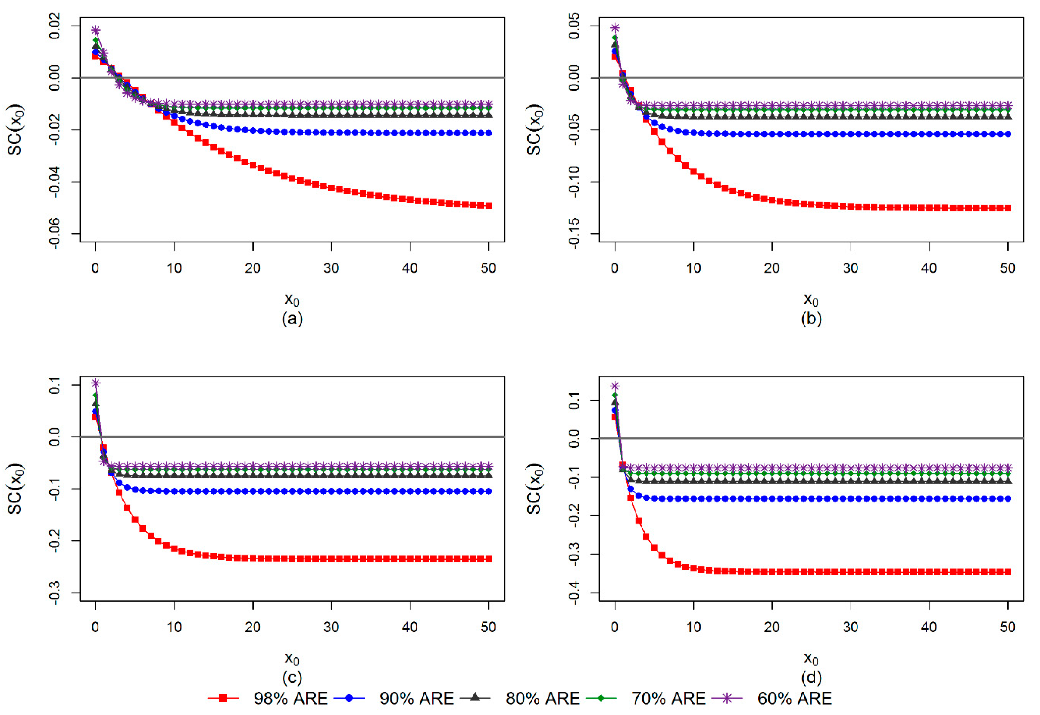
5.4. IF of PITS Estimator

According to Marona [35], the IF of an estimator is an asymptotic version of its sensitivity curve (SC). In general, the SC measures the sensitivity of an estimator to the location of the outlier $x_0$ for a particular random sample. Since using Equation (16) to obtain the IF of the PITS estimator is rather complicated, we apply its SC as an approximation of IF. The SC of the PITS estimator ${\widehat{\theta }}_{PITS}$ for the random sample $x_1,x_2,\dots ,x_n$ is defined as a function of the location of the outlier $x_0$, which can be written as follows:

$$\mathrm{SC}(x_0)={\widehat{\theta }}_{PITS}(x_1,x_2,\dots ,x_n,x_0)-{\widehat{\theta }}_{PITS}(x_1,x_2,\dots ,x_n).$$

(24)

where ${\widehat{\theta }}_{PITS}(x_1,x_2,\dots ,x_n)$ is the PITS estimator using the samples $x_1,x_2,\dots ,x_n$. To obtain the SC of the PITS estimator, we generated a random sample of size n = 50 from the Lindley distribution with parameter θ = 0.5, 1, 2, 3. Then, a single outlier $x_0$ is added to the sample data. The value of $x_0$ changed from 0 to 50 in increments of 1. Note that the 99th percentile are often used as upper boundaries for outlier identification, where any data point that exceed the 99th percentile can be considered as a potential outlier. For each parameter θ = 0.5, 1, 2 and 3, the 99th percentile of Lindley distribution are 12.4940, 5.9902, 2.8330 and 1.8222, respectively. Thus, the value of $x_0$ that exceed these 99th percentiles of Lindley distribution is large enough to be considered as a potential outlier. We obtained the $\mathrm{SC}(x_0)$ of the PITS estimator with several different AREs for each value of $x_0$, as shown in Figure 1.

Based on Figure 1, we can see that as $x_0$ increases, the SC of the PITS estimators with 98%, 90%, 80%, 70% and 60% AREs converge to a certain limit, which indicates that the curve is bounded. This suggests that the PITS estimator has a bounded IF and is robust against the location of a single outlier. As the level of ARE decreases, the limit of each curve moves closer to 0, which suggests that the PITS estimator becomes more robust.

6. Simulation Study

In this section, we investigate the performance of the ML, OLS, WLS and PITS (98%, 90%, 80%, 70% and 60% AREs) estimators in the absence and presence of outliers via a simulation study. In Section 6.1 and 6.2, we present the framework and results of the simulation study, respectively. Then, in Section 6.3, we provide some guidelines for selecting the appropriate ARE of the PITS estimator for practical application purposes.

6.1. Simulation Framework

The simulation procedure goes as follows:

Step 1:

Generate a random variable from the Lindley distribution for two sample size settings, that is, small (n = 30, 50, 70) and large (n = 100, 300, 500), with parameter θ = 0.5, 1, 2, 3.

Step 2:

Randomly select some observations and replace them with outliers generated from the Lindley distribution with parameter 0.05θ. Note that by multiplying the true value of parameter θ with 0.05, the Lindley distribution will have heavier upper tail and will produce larger values of random variables, which are interpreted as outliers. For the small sample sizes, generate outliers for several fixed numbers, m = 0, 1, 3, 5. For the large sample sizes, simulate outliers for several fixed proportions, ε = 0%, 1%, 5%, 10%.

Step 3:

Estimate the parameter θ using the ML, OLS, WLS and PITS (98%, 90%, 80%, 70% and 60% AREs) methods.

Step 4:

Repeat steps 1–3 10,000 times.

Step 5:

Calculate the performance of each estimator using the percentage relative root mean square error (RRMSE). For a given true value of parameter θ, the RRMSE is given by the following:

$$\mathrm{RRMSE}=\frac{100}{\theta }\sqrt{\frac{1}{N}{\displaystyle \sum _{i=1}^N{\left({\widehat{\theta }}_i-\theta \right)}^2}},$$

(25)

where ${\widehat{\theta }}_i$ is the estimated parameter for the i-th (i = 1, 2,…, N) sample and N is the number of simulated samples. A smaller RRMSE value indicates that the estimator is more accurate and precise. Thus, any estimation method that minimizes the RRMSE provides the best estimation of the parameter θ.

6.2. Simulation Results

Table 3. Relative root mean square error (RRMSE) results for estimations of parameter θ with n = 30 and m = 0, 1, 3, 5.

θ	m	RRMSE
		ML	OLS	WLS	PITS 98% ARE	PITS 90% ARE	PITS 80% ARE	PITS 70% ARE	PITS 60% ARE
0.5	0	14.02	15.42	14.94	14.01	14.24	14.82	15.61	16.66
	1	38.97	15.51	15.08	18.71	14.48	14.55	15.18	16.14
	3	64.24	17.55	17.83	46.07	24.03	19.23	17.76	17.60
	5	74.95	22.53	22.81	67.20	38.26	27.91	23.87	21.70
1	0	14.56	16.17	15.62	14.56	14.91	15.64	16.60	17.89
	1	39.91	16.05	15.75	19.19	15.03	15.27	16.10	17.32
	3	64.71	18.25	18.59	46.66	24.66	19.85	18.42	18.40
	5	75.36	23.46	23.86	67.58	39.14	28.70	24.66	22.60
2	0	15.52	17.37	16.69	15.52	16.01	16.89	18.04	19.58
	1	41.21	17.47	16.83	20.13	15.97	16.37	17.37	18.82
	3	65.80	19.58	19.94	47.84	25.92	21.05	19.60	19.70
	5	76.22	25.00	25.49	68.11	40.61	30.08	25.99	24.06
3	0	16.27	18.26	17.50	16.26	16.78	17.76	19.07	20.82
	1	42.41	18.35	17.64	20.44	16.34	16.88	18.07	19.75
	3	66.83	20.03	20.31	48.52	26.36	21.37	20.10	20.23
	5	76.60	25.71	26.28	68.37	41.44	30.77	26.63	24.69

The best method for each case is written in bold.

,

Table 4. RRMSE results for estimations of parameter θ with n = 50 and m = 0, 1, 3, 5.

θ	m	RRMSE
		ML	OLS	WLS	PITS 98% ARE	PITS 90% ARE	PITS 80% ARE	PITS 70% ARE	PITS 60% ARE
0.5	0	10.63	11.66	11.30	10.63	10.81	11.24	11.82	12.60
	1	29.44	11.73	11.41	12.97	10.94	11.13	11.64	12.38
	3	52.62	12.76	12.94	28.73	15.72	13.37	12.80	12.90
	5	64.76	15.52	15.91	45.84	23.49	17.93	15.95	15.03
1	0	11.13	12.36	11.89	11.14	11.42	11.96	12.66	13.58
	1	30.03	12.45	12.05	13.21	11.37	11.72	12.38	13.27
	3	53.48	13.30	13.48	29.30	16.11	13.84	13.39	13.73
	5	65.42	16.04	16.51	46.39	23.90	18.31	16.42	15.42
2	0	11.66	13.14	12.59	11.68	12.10	12.77	13.61	14.70
	1	31.98	13.22	12.71	13.99	12.10	12.54	13.32	14.36
	3	55.12	14.27	14.47	30.48	17.08	14.78	14.40	14.94
	5	66.69	17.29	17.84	47.71	25.26	19.53	17.61	16.73
3	0	12.23	13.93	13.28	12.25	12.77	13.55	14.51	15.73
	1	32.77	14.02	13.39	14.42	12.64	13.21	14.11	15.30
	3	55.81	14.94	15.11	31.06	17.62	15.38	15.05	15.57
	5	67.58	17.88	18.45	48.36	25.87	20.07	18.17	17.05

The best method for each case is written in bold.

,

Table 5. RRMSE results for estimations of parameter θ with n = 70 and m = 0, 1, 3, 5.

θ	m	RRMSE
		ML	OLS	WLS	PITS 98% ARE	PITS 90% ARE	PITS 80% ARE	PITS 70% ARE	PITS 60% ARE
0.5	0	8.88	9.80	9.46	8.89	9.07	9.44	9.92	10.57
	1	55.91	9.87	9.56	10.69	9.16	9.37	9.81	10.43
	3	79.24	10.52	10.61	23.47	12.35	10.81	10.56	10.91
	5	86.74	12.21	12.55	39.28	17.67	13.69	12.46	11.91
1	0	9.29	10.36	9.95	9.30	9.56	10.01	10.57	11.30
	1	56.68	10.42	10.04	11.11	9.62	9.91	10.44	11.14
	3	79.67	11.06	11.15	24.22	12.85	11.31	11.10	11.51
	5	87.03	12.98	13.29	40.34	18.36	14.31	13.09	12.79
2	0	9.72	11.00	10.51	9.74	10.10	10.68	11.41	12.34
	1	58.04	11.06	10.61	11.59	10.11	10.53	11.21	12.12
	3	80.51	11.69	11.79	25.33	13.48	11.94	11.74	12.39
	5	87.30	13.88	14.13	41.95	19.27	15.08	13.88	13.68
3	0	10.22	11.53	10.99	10.23	10.60	11.22	11.99	12.98
	1	59.02	11.60	11.08	11.92	10.50	10.99	11.73	12.70
	3	81.13	12.18	12.26	26.09	13.93	12.40	12.22	12.99
	5	87.76	14.30	14.64	43.13	19.87	15.58	14.38	14.21

The best method for each case is written in bold.

,

Table 6. RRMSE results for estimations of parameter θ with n = 100 and ε = 0%, 1%, 5%, 10%.

θ	ε (%)	RRMSE
		ML	OLS	WLS	PITS 98% ARE	PITS 90% ARE	PITS 80% ARE	PITS 70% ARE	PITS 60% ARE
0.5	0	7.34	8.15	7.86	7.35	7.51	7.85	8.28	8.84
	1	18.48	8.19	7.92	8.23	7.56	7.83	8.23	8.78
	5	48.82	9.63	9.89	23.91	12.64	10.38	9.66	9.75
	10	65.36	13.77	14.27	45.56	22.86	16.75	14.31	13.03
1	0	7.70	8.56	8.23	7.71	7.92	8.30	8.78	9.41
	1	19.23	8.60	8.28	8.57	7.95	8.25	8.70	9.32
	5	49.74	10.05	10.35	24.53	13.06	10.78	10.10	10.22
	10	66.05	14.52	15.12	46.34	23.63	17.41	14.95	13.60
2	0	8.21	9.26	8.85	8.22	8.54	9.01	9.59	10.32
	1	20.65	9.30	8.90	9.05	8.54	8.93	9.49	10.21
	5	51.52	10.88	11.20	25.60	13.86	11.56	10.98	11.13
	10	67.26	15.63	16.31	47.55	24.80	18.45	15.96	14.68
3	0	8.61	9.72	9.25	8.63	8.95	9.46	10.10	10.90
	1	21.45	9.75	9.29	9.36	8.88	9.33	9.95	10.75
	5	52.70	11.26	11.58	26.22	14.27	11.94	11.34	11.58
	10	68.16	16.23	16.97	48.34	25.53	19.06	16.52	15.28

The best method for each case is written in bold.

,

Table 7. RRMSE results for estimations of parameter θ with n = 300 and ε = 0%, 1%, 5%, 10%.

θ	ε (%)	RRMSE
		ML	OLS	WLS	PITS 98% ARE	PITS 90% ARE	PITS 80% ARE	PITS 70% ARE	PITS 60% ARE
0.5	0	4.25	4.75	4.56	4.26	4.37	4.57	4.81	5.11
	1	17.25	4.81	4.71	6.09	4.70	4.69	4.86	5.13
	5	49.24	7.41	7.85	23.64	11.57	8.67	7.47	7.07
	10	65.80	12.63	13.18	45.57	22.60	16.06	13.23	11.58
1	0	4.40	4.86	4.67	4.40	4.51	4.72	4.98	5.33
	1	18.14	4.92	4.83	6.26	4.84	4.83	5.02	5.33
	5	50.26	7.77	8.28	24.27	11.97	9.00	7.82	7.38
	10	66.48	13.31	13.97	46.26	23.28	16.64	13.77	12.10
2	0	4.68	5.24	5.00	4.69	4.84	5.10	5.42	5.82
	1	19.58	5.34	5.22	6.73	5.26	5.26	5.49	5.84
	5	52.02	8.50	9.08	25.36	12.79	9.72	8.54	8.07
	10	67.74	14.49	15.27	47.57	24.59	17.77	14.82	13.10
3	0	4.83	5.45	5.18	4.84	5.02	5.30	5.64	6.08
	1	20.30	5.51	5.36	6.85	5.39	5.42	5.68	6.07
	5	53.22	8.76	9.39	25.93	13.13	9.99	8.80	8.34
	10	68.63	14.99	15.85	48.30	25.26	18.31	15.29	13.53

The best method for each case is written in bold.

and

Table 8. RRMSE results for estimations of parameter θ with n = 500 and ε = 0%, 1%, 5%, 10%.

θ	ε (%)	RRMSE
		ML	OLS	WLS	PITS 98% ARE	PITS 90% ARE	PITS 80% ARE	PITS 70% ARE	PITS 60% ARE
0.5	0	3.25	3.62	3.48	3.26	3.34	3.48	3.67	3.91
	1	16.98	3.75	3.71	5.53	3.80	3.71	3.79	3.98
	5	49.32	6.89	7.37	23.56	11.34	8.29	7.00	6.41
	10	65.89	12.38	12.93	45.53	22.51	15.90	12.99	11.21
1	0	3.36	3.75	3.59	3.36	3.46	3.63	3.84	4.11
	1	17.89	3.91	3.87	5.78	4.01	3.88	3.98	4.19
	5	50.46	7.31	7.89	24.28	11.82	8.69	7.39	6.78
	10	66.57	13.14	13.82	46.32	23.29	16.57	13.61	11.80
2	0	3.55	4.02	3.82	3.57	3.70	3.90	4.14	4.45
	1	19.29	4.19	4.13	6.09	4.26	4.15	4.28	4.52
	5	52.23	7.88	8.54	25.28	12.49	9.24	7.90	7.27
	10	67.82	14.16	14.97	47.49	24.46	17.55	14.51	12.67
3	0	3.71	4.23	4.02	3.73	3.89	4.12	4.39	4.73
	1	20.11	4.40	4.33	6.32	4.49	4.35	4.52	4.79
	5	53.42	8.25	8.96	25.95	12.95	9.62	8.27	7.61
	10	68.70	14.81	15.68	48.30	25.25	18.21	15.10	13.20

The best method for each case is written in bold.

list the results of the simulation study based on the obtained RRMSEs. We summarize these results as follows:

• In the cases of both small and large sample sizes (Table 3, Table 4, Table 5, Table 6, Table 7 and Table 8), we found the following:
  • When there are no outliers (m = 0 and ε = 0%) in the data, both the ML and PITS (98% ARE) estimators perform similarly and slightly outperform the OLS and WLS estimators.
  • In the presence of outliers, the performance of the ML estimator is much worse than that of the other estimators. As the degree of contamination increases, the performance of the ML estimator deteriorates significantly.
  • The OLS and WLS estimators are quite robust and offer some protection against outliers.
  • As the sample size increases, for all the cases considered, the performance of all the estimators improve, with the RRMSE values becoming smaller.
• In the case of a small sample size (Table 3, Table 4 and Table 5), we found the following:
  • When the number of outliers is small (m = 1), the PITS (90% ARE) estimator performs best, that is, slightly better than the OLS and WLS estimators.
  • When the number of outliers is moderate (m = 3), the OLS, WLS and PITS (70% and/or 60% AREs) estimators perform almost equally well and are considered to be the best methods for this particular case.
  • When the number of outliers is large (m = 5), the PITS (60% ARE) estimator performs best, that is, slightly better than the OLS and WLS estimators.
• In the case of a large sample size (Table 6, Table 7 and Table 8), we found the following:
  • When the proportion of outliers is small (ε = 1%), for n = 100, the PITS (90% ARE) estimator performs best, that is, slightly better than the OLS and WLS estimators. For n = 300, 500, the OLS, WLS and PITS (90% and 80% AREs) estimators perform almost equally well and are considered to be the best methods for this particular case.
  • When the proportion of outliers is moderate (ε = 5%), for n = 100, the OLS and PITS (70% ARE) estimators perform very similarly, slightly outperforming the WLS estimator. For n = 300, 500, the PITS (60% ARE) estimator performs best, outperforming all the other methods.
  • When the proportion of outliers is large (ε = 10%), the performance of the PITS (60% ARE) estimator also surpasses that of other methods.

Overall, in the presence of outliers, the use of the ML estimator should be avoided since it is not robust and provides no protection against outliers. It is also interesting to note that we found the OLS and WLS estimators to be quite robust and able to offer some protection against outliers. However, the proposed PITS estimator provides the most flexible approach as it can be applied in both the absence and presence of outliers.

6.3. Some Guidelines for Selecting the Appropriate ARE of PITS Estimator

Based on the results of a comprehensive simulation study, here we provide some guidelines for selecting the appropriate ARE of PITS estimator in practical application:

• When there are no outliers in the data, the PITS (98% ARE) estimator should be applied for estimating parameter θ.
• For small sample size setting, that is, n < 30:
  • When number of outliers m ≤ 3, the PITS (60–90% AREs) estimators are preferable for estimating parameter θ.
  • When number of outliers m ≥ 4, the PITS (50–60% AREs) estimators are preferable for estimating parameter θ.
• For small sample size setting, that is, 30 ≤ n ≤ 70:
  • When number of outliers m ≤ 2, the PITS (80–90% AREs) estimators are recommended for estimating parameter θ.
  • When number of outliers 3 ≤ m ≤ 4, the PITS (60–80% AREs) estimators are preferable for estimating parameter θ.
  • When number of outliers m ≥ 5, the PITS (50–60% AREs) estimators are recommended for estimating parameter θ.
• For large sample size setting, that is, 70 < n ≤ 100:
  • When number of outliers m ≤ 3, the PITS (70–90% AREs) estimators are recommended for estimating parameter θ.
  • When number of outliers 4 ≤ m ≤ 6, the PITS (60–70% AREs) estimators are recommended for estimating parameter θ.
  • When number of outliers m ≥ 7, the PITS (50–60% AREs) estimators are preferable for estimating parameter θ.
• For large sample size setting, that is, n > 100:
  • When proportion of outliers ε ≤ 3%, the PITS (80–90% AREs) estimators are preferable for estimating parameter θ.
  • When proportion of outliers 3% < ε ≤ 7%, the PITS (60–80% AREs) estimators are preferable for estimating parameter θ.
  • When proportion of outliers ε > 7%, the PITS (50–60% AREs) estimators are recommended for estimating parameter θ.

7. Applications and Discussion

In this section, we report four applications of the Lindley distribution as a reliability model using real data sets and compare the performance of the ML, OLS, WLS and PITS (with several AREs) estimators. Note that the AREs of PITS estimator are determined based on the proportion of outliers found in the data. The first data set (Data Set 1) consists of the time to failure of 18 electronic devices reported by Wang [36]. The second data set (Data Set 2) represents the survival times of 44 patients suffering from head and neck cancers (treated using radiotherapy and chemotherapy), which were initially reported by Efron [37] (see also Reference [38]). The third data set (Data Set 3) consists of an uncensored data set of the remission times of a random sample of 128 bladder cancer patients, which was obtained from Lee and Wang [5]. Finally, the fourth data set (Data Set 4) represents the length of stay of 300 patients suffering from breast cancer, which can be found in Reference [39]. All four data sets are given in Appendix A.

For all the data sets considered, to identify the presence of outliers, we applied the generalized boxplot method [40], which is suitable for skewed and/or heavy-tailed distributions. In practical applications, we suggest to apply this method for the purpose of outlier detection for the data that follows the Lindley distribution.

Table 9. Descriptive statistics for data Sets 1, 2, 3 and 4.

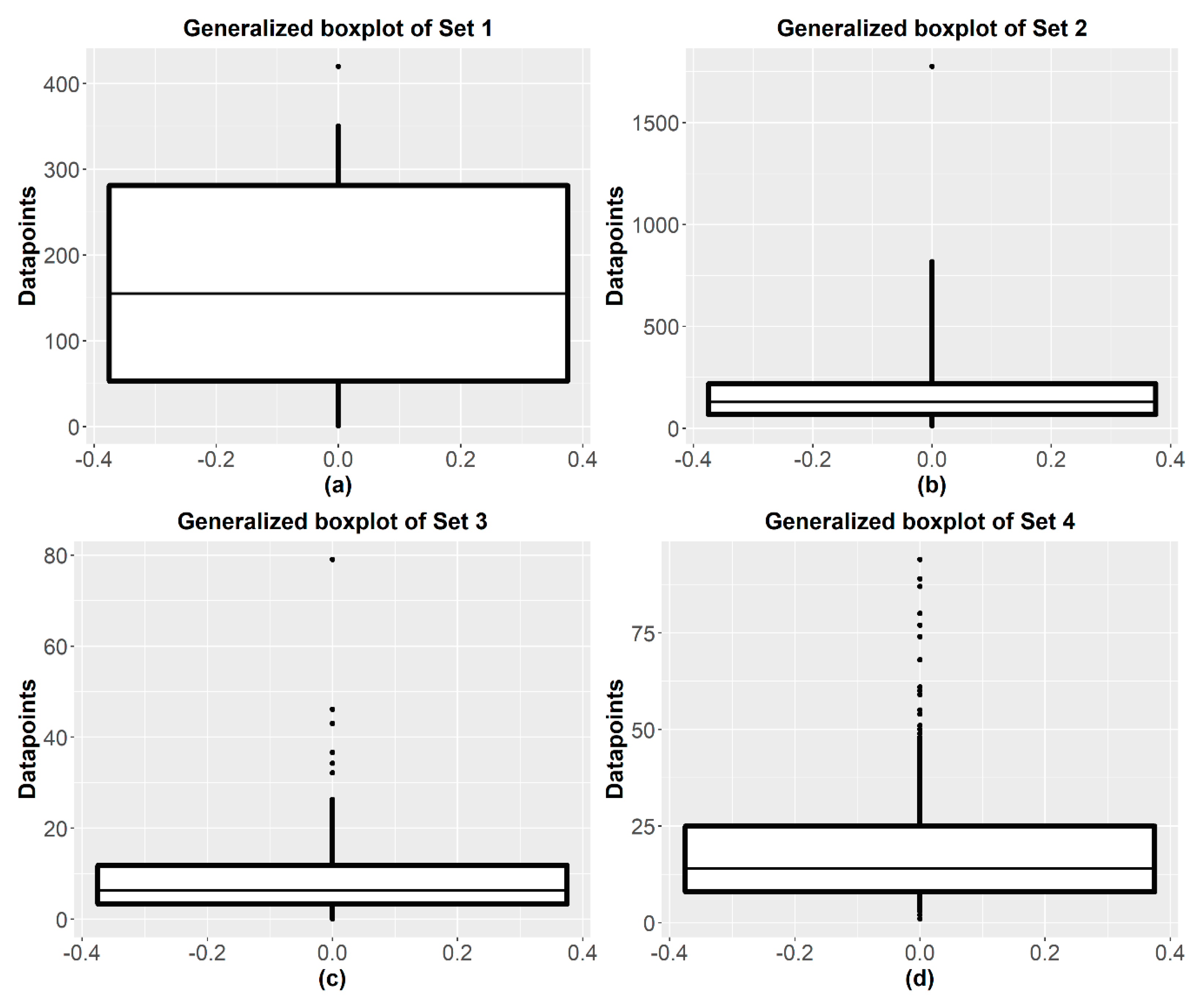
Set	Sample Size (n)	Mean	Median	Min	Max	Std. Deviation	Skewness	No. of Outliers (Proportion)
Set 1	18	171.50	155.00	1.00	420.00	132.27	0.28	1 (5.55%)
Set 2	44	223.48	128.50	12.20	1776.00	305.43	3.27	1 (2.27%)
Set 3	128	9.37	6.40	0.08	79.05	10.51	3.25	6 (4.69%)
Set 4	300	18.44	14.00	1.00	94.00	15.89	1.96	17 (5.67%)

provides descriptive statistics for all the data sets and Figure 2 shows generalized boxplots of these data sets.

To compare the performance of the considered methods in estimating the parameter of the Lindley distribution, we applied the Kolmogorov-Smirnov (K-S) test, Akaike information criterion (AIC) and Bayesian information criterion (BIC) to assess goodness of fit. The best method is determined by that yielding the highest p-value of the K-S test and the smallest value of K-S statistic, AIC and BIC.

Table 10. Parameter estimates and goodness of fits of the Lindley distributions of data Sets 1, 2, 3 and 4.

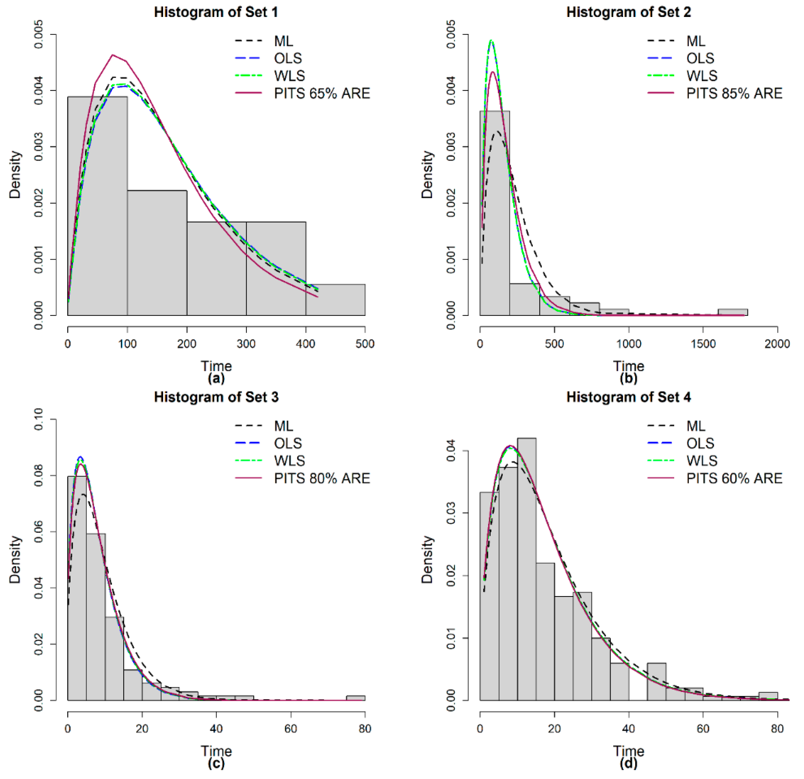
Data	Method	Estimated Parameter $(\widehat{\mathit{\theta }})$	K-S Statistic	p-Value	AIC	BIC
Set 1	ML	0.01160	0.1737	0.5895	230.7422	231.6326
	OLS	0.01115	0.1802	0.5434	230.7963	231.6867
	WLS	0.01127	0.1786	0.5550	230.7720	231.6623
	PITS (75% ARE)	0.01180	0.1707	0.6112	230.7532	231.6435
	PITS (70% ARE)	0.01214	0.1655	0.6483	230.8193	231.7097
	PITS (65% ARE)	0.01261	0.1641	0.6583	231.0041	231.8945
	PITS (60% ARE)	0.01324	0.1866	0.4998	231.4050	232.2954
Set 2	ML	0.00891	0.2194	0.0243	581.1628	582.9470
	OLS	0.01325	0.1374	0.3453	597.0666	598.8508
	WLS	0.01333	0.1380	0.3404	597.5451	599.3293
	PITS (95% ARE)	0.01035	0.1510	0.2425	583.2425	585.0267
	PITS (90% ARE)	0.01117	0.1225	0.4864	586.0117	587.7959
	PITS (85% ARE)	0.01178	0.1220	0.4916	588.7263	590.5104
	PITS (80% ARE)	0.01227	0.1280	0.4306	591.2379	593.0220
Set 3	ML	0.19605	0.1164	0.0623	841.0598	843.9118
	OLS	0.23028	0.0597	0.7509	847.9594	850.8115
	WLS	0.22761	0.0580	0.7826	846.9738	849.8258
	PITS (80% ARE)	0.22368	0.0555	0.8247	845.6468	848.4988
	PITS (75% ARE)	0.22635	0.0571	0.7977	846.5308	849.3828
	PITS (70% ARE)	0.22852	0.0586	0.7718	847.2994	850.1514
	PITS (65% ARE)	0.23032	0.0598	0.7504	847.8874	850.7394
Set 4	ML	0.10338	0.0772	0.0558	2326.7150	2330.4190
	OLS	0.10998	0.0439	0.6099	2329.0490	2332.7520
	WLS	0.10922	0.0476	0.5049	2328.5550	2332.2590
	PITS (75% ARE)	0.10929	0.0472	0.5152	2328.6020	2332.3060
	PITS (70% ARE)	0.10973	0.0451	0.5753	2328.8820	2332.5860
	PITS (65% ARE)	0.11012	0.0432	0.6306	2329.1500	2332.8540
	PITS (60% ARE)	0.11039	0.0419	0.6673	2329.3420	2333.0460

The best method is written in bold.

lists the estimated parameters and goodness of fits obtained for the Lindley distribution for all the data sets. As presented in Table 10, we can observe that the PITS estimator provides a better estimation of the Lindley parameter than the ML, OLS and WLS estimators based on its smallest K-S statistic and highest p-value of the K-S test. On the other hand, the ML estimator is found to be the best method for estimating the parameter θ based on its smallest value of AIC and BIC. This is because the ML estimator maximized the likelihood function of the Lindley model and as a result the AIC and BIC will always favor the ML estimator. Thus, in our case here, we could say that the AIC and BIC are biased measures for goodness of fit assessment. To further support our claim regarding the AIC and BIC, we provide another example where the data is simulated from Lindley distribution with θ = 2 for sample size n = 100. Then, we random select 5% of the observations and replace them with outliers. Based on this data, we compare the performances of all methods in estimating the parameter of the Lindley distribution. The K-S test, AIC and BIC are utilized to assess goodness of fit. The result of the comparative study is presented in

Table 11. Parameter estimates and goodness of fits of Lindley distribution for simulated data from Lindley distribution with θ = 2, n = 100 and 5% outliers.

Method	Estimated Parameter $(\widehat{\mathit{\theta }})$	K-S Statistic	p-Value	AIC	BIC
ML	0.81958	0.4256	<0.0001	401.3450	403.9502
OLS	2.06962	0.0618	0.8383	608.0914	610.6965
WLS	2.04933	0.0610	0.8505	603.0340	605.6391
PITS (90% ARE)	1.92935	0.0658	0.7784	573.7682	576.3734
PITS (85% ARE)	1.98865	0.0581	0.8875	588.0901	590.6952
PITS (80% ARE)	2.02738	0.0600	0.8638	597.5959	600.2011
PITS (75% ARE)	2.05503	0.0612	0.8471	604.4503	607.0555
PITS (70% ARE)	2.07697	0.0621	0.8340	609.9304	612.5355
PITS (65% ARE)	2.09547	0.0629	0.8232	614.5775	617.1827

The best method is written in bold.

.

Based on the result from Table 11, it can be seen that the estimated parameter found based on ML estimator ($\widehat{\theta }$ = 0.81958) is much deviated from the true value of θ = 2. However, if the AIC and BIC are used for determining the best model, it can be observed that the best fitted Lindley distribution is found when the parameter θ is estimated using ML estimator. This further support our claim that AIC and BIC will always favor the ML estimator although the outliers are present in the data. On the other hand, K-S statistic and p-value of K-S test are able to determine the best method for estimating the parameter θ which is PITS (85% ARE). Since the AIC and BIC would provide a biased measures for goodness of fit assessment, thus, in this study, the best Lindley model is only determined based on the smallest value of K-S statistic and the highest p-value of K-S test.

As we mentioned before, based on the smallest K-S statistic and highest p-value of the K-S test, the PITS estimator is found to provide a better estimation of the Lindley parameter than the ML, OLS and WLS estimators. This result is supported by the fitted PDF shown in Figure 3. In addition, due to the substantial increase in the p-value of the K-S test, we note that the fittings of the Lindley distribution for data Sets 2, 3 and 4 are significantly improved when the PITS estimator is used to estimate parameter θ, as compared to the ML estimator. This is due to the presence of outliers far beyond the rest of the data, as shown in Figure 3b–d. However, the OLS and WLS estimators are also found to be quite reliable for estimating parameter θ despite the presence of outliers in the data.

Since the reliability measures based on the Lindley distribution depend on parameter θ, it is important to employ the most suitable method for estimating parameter θ. Based on its application to real data sets, we have shown that the proposed PITS estimator is a viable alternative for estimating the parameter of the Lindley distribution especially when outliers are present in the data.

8. Conclusions

In this paper, we proposed a new robust and efficient estimator of the parameter of the Lindley distribution based on the PITS. The advantage of the PITS estimator is that it is conceptually simple and easy to compute. An assessment of the robustness of the PITS estimator based on the BP and IF revealed that the PITS estimator has a high BP and bounded IF, which means that this estimator offers reasonable protection against outliers. In a simulation study, we compared the performance of the PITS estimator with those of several well-known estimators, namely ML, OLS and WLS. The results of the simulation indicated that the performance of the PITS estimator was similar to that of the ML estimator in the absence of outliers and outperforms all the other methods in the presence of outliers. We also note that the OLS and WLS estimators are quite robust and outperformed the ML estimator in the presence of outliers. Four real data sets were applied for which the parameter of the Lindley distribution was estimated. The results demonstrated that the PITS estimator provides a better fitting of this model than the other methods in terms of smallest K-S statistic and highest p-value of the K-S test. Finally, all the abbreviations are listed in Abbreviations part and the R commands for the PITS estimator are available in Appendix B.

References

- IEEE. IEEE Standard Computer Dictionary: A Compilation of IEEE Standard Computer Glossaries; IEEE Std 610; IEEE Press: New York, NY, USA, 1991; pp. 1–217. [Google Scholar]
- Murthy, D.N.P.; Rausand, M.; Østerås, T. Product Reliability: Specification and Performance; Springer: London, UK, 2008. [Google Scholar]
- Meeker, W.Q.; Escobar, L.A. Statistical Methods for Reliability Data; John Wiley & Sons: New York, NY, USA, 2014. [Google Scholar]
- Blischke, W.R.; Murthy, D.N.P. Reliability: Modeling, Prediction, and Optimization; John Wiley & Sons: New York, NY, USA, 2000. [Google Scholar]
- Lee, E.T.; Wang, J. Statistical Methods for Survival Data Analysis, 3rd ed.; John Wiley & Sons: New York, NY, USA, 2003; Volume 476. [Google Scholar]
- Ghitany, M.E.; Atieh, B.; Nadarajah, S. Lindley distribution and its application. Math. Comput. Simul. 2008, 78, 493–506. [Google Scholar] [CrossRef]
- Krishna, H.; Kumar, K. Reliability estimation in Lindley distribution with progressively type II right censored sample. Math. Comput. Simul. 2011, 82, 281–294. [Google Scholar] [CrossRef]
- Lindley, D.V. Fiducial Distributions and Bayes’ Theorem. J. R. Stat. Soc. Ser. B 1958, 20, 102–107. [Google Scholar] [CrossRef]
- Nie, J.; Gui, W. Parameter estimation of Lindley distribution based on progressive type-II censored competing risks data with binomial removals. Mathematics 2019, 7, 646. [Google Scholar] [CrossRef]
- Ghitany, M.E.; Alqallaf, F.; Al-Mutairi, D.K.; Husain, H.A. A two-parameter weighted Lindley distribution and its applications to survival data. Math. Comput. Simul. 2011, 81, 1190–1201. [Google Scholar] [CrossRef]
- Nadarajah, S.; Bakouch, H.S.; Tahmasbi, R. A generalized Lindley distribution. Sankhya B 2011, 73, 331–359. [Google Scholar] [CrossRef]
- Bakouch, H.S.; Al-Zahrani, B.M.; Al-Shomrani, A.A.; Marchi, V.A.A.; Louzada, F. An extended Lindley distribution. J. Korean Stat. Soc. 2012, 41, 75–85. [Google Scholar] [CrossRef]
- Ghitany, M.E.; Al-Mutairi, D.K.; Balakrishnan, N.; Al-Enezi, L.J. Power Lindley distribution and associated inference. Comput. Stat. Data Anal. 2013, 64, 20–33. [Google Scholar] [CrossRef]
- Oluyede, B.O.; Yang, T. A new class of generalized Lindley distributions with applications. J. Stat. Comput. Simul. 2015, 85, 2072–2100. [Google Scholar] [CrossRef]
- Ashour, S.K.; Eltehiwy, M.A. Exponentiated power Lindley distribution. J. Adv. Res. 2015, 6, 895–905. [Google Scholar] [CrossRef]
- Asgharzadeh, A.; Bakouch, H.S.; Nadarajah, S.; Sharafi, F. A new weighted lindley distribution with application. Brazilian J. Probab. Stat. 2016, 30, 1–27. [Google Scholar] [CrossRef]
- Kemaloglu, S.A.; Yilmaz, M. Transmuted two-parameter Lindley distribution. Commun. Stat. Theory Methods 2017, 46, 11866–11879. [Google Scholar] [CrossRef]
- MirMostafaee, S.M.T.K.; Alizadeh, M.; Altun, E.; Nadarajah, S. The exponentiated generalized power Lindley distribution: Properties and applications. Appl. Math. 2019, 34, 127–148. [Google Scholar] [CrossRef]
- Barnett, V.; Lewis, T. Outliers in Statistical Data, 3rd ed.; Wiley: New York, NY, USA, 1994. [Google Scholar]
- Huber, S. (Non-)robustness of maximum likelihood estimators for operational risk severity distributions. Quant. Financ. 2010, 10, 871–882. [Google Scholar] [CrossRef]
- Ahmed, E.S.; Volodin, A.I.; Hussein, A.A. Robust weighted likelihood estimation of exponential parameters. IEEE Trans. Reliab. 2005, 54, 389–395. [Google Scholar] [CrossRef]
- Shahriari, H.; Radfar, E.; Samimi, Y. Robust estimation of systems reliability. Qual. Technol. Quant. Manag. 2017, 14, 310–324. [Google Scholar] [CrossRef]
- Boudt, K.; Caliskan, D.; Croux, C. Robust explicit estimators of Weibull parameters. Metrika 2011, 73, 187–209. [Google Scholar] [CrossRef]
- Adatia, A. Robust estimators of the 2-parameter gamma distribution. IEEE Trans. Reliab. 1988, 37, 234–238. [Google Scholar] [CrossRef]
- Marazzi, A.; Ruffieux, C. Implementing M-Estimators of the Gamma Distribution. In Robust Statistics, Data Analysis, and Computer Intensive Methods: In Honor of Peter Huber’s 60th Birthday; Rieder, H., Ed.; Springer: New York, NY, USA, 1996; pp. 277–297. [Google Scholar]
- Clarke, B.R.; McKinnon, P.L.; Riley, G. A fast robust method for fitting gamma distributions. Stat. Pap. 2012, 53, 1001–1014. [Google Scholar] [CrossRef]
- Serfling, R. Efficient and robust fitting of lognormal distributions. N. Am. Actuar. J. 2002, 6, 95–109. [Google Scholar] [CrossRef]
- Quesenberry, C.P. Probability integral transformations. Encycl. Stat. Sci. 2004, 10. [Google Scholar] [CrossRef]
- Finkelstein, M.; Tucker, H.G.; Alan Veeh, J. Pareto tail index estimation revisited. North Am. Actuar. J. 2006, 10, 1–10. [Google Scholar] [CrossRef]
- Safari, M.A.M.; Masseran, N.; Ibrahim, K.; Hussain, S.I. A robust and efficient estimator for the tail index of inverse Pareto distribution. Phys. A Stat. Mech. Its Appl. 2019, 517, 431–439. [Google Scholar] [CrossRef]
- Safari, M.A.M.; Masseran, N.; Ibrahim, K.; AL-Dhurafi, N.A. The power-law distribution for the income of poor households. Phys. A Stat. Mech. Its Appl. 2020, 557, 124893. [Google Scholar] [CrossRef]
- Jodrá, P. Computer generation of random variables with Lindley or Poisson-Lindley distribution via the Lambert W function. Math. Comput. Simul. 2010, 81, 851–859. [Google Scholar] [CrossRef]
- Huber, P.J. Robust Statistics; John Wiley & Sons: New York, NY, USA, 1981. [Google Scholar]
- Hampel, F.R.; Ronchetti, E.M.; Rousseeuw, P.J.; Stahel, W.A. Robust Statistics: The Approach Based on Influence Functions; John Wiley & Sons: New York, NY, USA, 1986. [Google Scholar]
- Maronna, R.A.; Martin, R.D.; Yohai, V.J.; Salibián-Barrera, M. Robust Statistics: Theory and Methods (with R), 2nd ed.; John Wiley & Sons: Chichester, UK, 2019. [Google Scholar]
- Wang, F.K. A new model with bath tub-shaped failure rate using an additive Burr XII distribution. Reliab. Eng. Syst. Saf. 2000, 70, 305–312. [Google Scholar] [CrossRef]
- Efron, B. Logistic regression, survival analysis, and the Kaplan-Meier curve. J. Am. Stat. Assoc. 1988, 83, 414–425. [Google Scholar] [CrossRef]
- Sharma, V.K.; Singh, S.K.; Singh, U.; Agiwal, V. The inverse Lindley distribution: A stress-strength reliability model with application to head and neck cancer data. J. Ind. Prod. Eng. 2015, 32, 162–173. [Google Scholar] [CrossRef]
- Adamu, P.I.; Oguntunde, P.E.; Okagbue, H.I.; Agboola, O.O. Statistical data analysis of cancer incidences in insurgency affected states in Nigeria. Data Br. 2018, 18, 2029–2046. [Google Scholar] [CrossRef]
- Bruffaerts, C.; Verardi, V.; Vermandele, C. A generalized boxplot for skewed and heavy-tailed distributions. Stat. Probab. Lett. 2014, 95, 110–117. [Google Scholar] [CrossRef]