Article

Modelling of Alumina Splat Solidification on Preheated Steel Substrate Using the Network Simulation Method

1
Department of Mechanical Engineering, Materials and Manufacturing, Universidad Politécnica de Cartagena, 30202 Cartagena, Spain
2
Department of Applied Physics and Naval Technology, Universidad Politécnica de Cartagena, 30202 Cartagena, Spain
3
Institute for Manufacturing Technologies of Ceramic Components and Composites (IMTCCC), University of Stuttgart, Allmandring 7b, 70569 Stuttgart, Germany
*
Author to whom correspondence should be addressed.
Mathematics 2020, 8(9), 1568; https://doi.org/10.3390/math8091568
Submission received: 16 August 2020 / Revised: 3 September 2020 / Accepted: 8 September 2020 / Published: 11 September 2020

Abstract

:
A mathematical model, consisting of a set of differential equations, for the simulation of the alumina splat solidification on steel substrate is presented. The network simulation method is used to solve the problem, which provides the temperatures and the cooling rate in the splat and substrate with a high temporal and spatial resolution for different values of the preheated substrate temperature. The results of this calculation provide important information for the design of ceramic coatings. The model design is explained in depth and simulated in open source software. As expected, the temperature evolutions in several points of the splat, an important variable to know the type of phases and the effect of the manufacturing parameters on this process, coincide with the experimental results. The model is also checked by another experimental test with tin and a bigger splat, which enables the temperature to be measured during solidification. It is worth highlighting the study of the cooling rate, a fundamental parameter to determine the phase, whether amorphous, gamma or alpha. Furthermore, a sensitive study of the mesh was included in order to optimize the computational time.

1. Introduction

Thermal spraying is a technique in which small molten particles of metals, alloys or ceramics (tens of μm) are sprayed at high speed (above 100 ms−1) onto a substrate creating a protective coating. One of these thermal spraying processes is the atmospheric plasma spray (APS). The mechanisms involved in the flattening are described in several studies where the different variables that can affect the final form of splat are analysed [1,2,3].
After impact, the particles solidify on the substrate producing thin and dense lamellae or layers, called splats, whose shape depends on the size, shape and powder material properties, flying particle temperature and impact velocity and roughness and temperature of the substrate, in short, heat transfer and flow fluid. The coating’s main characteristics, the adhesion strength on the substrate and the residual stresses generated at the interface depend on these properties [1,4,5,6,7,8,9,10,11,12,13,14,15,16].
Therefore, it is necessary to develop a deep understanding of the physical principles involved in the spread and solidification of the droplet, in order for the spraying process parameters, coating adhesion strength and splat morphology to be correlated and, as a result, the coating quality can be controlled [17].
With regard to the solidification, the cooling rate (CR) determines the phase in the solidified splat. Thus, the models developed by de Levi et al. provided the following results: an amorphous phase with a cooling rate around 105 K/s; a gamma phase with slower cooling rates; and finally, an alpha phase with a cooling rate in the range from 1 to 100 K/s [18]. On the other hand, several unidimensional analytical models show that the CR depends on [19,20,21,22,23]: the contact between the splat and the substrate, the melting latent heat, the relationship between the thermal diffusivities of the substrate and the splat and the inverse of splat thickness. Sobolev et al. obtained similar results with a simplified model [24,25].
The interface, which is usually defined by the inverse of the heat transfer coefficient in the interface, called contact thermal resistance, Rth, also depends on the absorbates and condensates in the substrate surface and also has an influence on the CR [26,27,28,29,30,31,32,33]. These products can disappear if preheating is applied on the substrate surface before the coating process. Yang et al. [34] have also evaluated the effect of substrate preheating on the splat grain structure. Fukumoto et al. [35] investigated the fractional change of the disk splat with an increase in the substrate temperature as well as the microstructure of the cross section of the splats using Y2O3, YSZ and Al2O3 powder materials that were plasma sprayed on an AISI304 stainless steel substrate.
After establishing that the phases in the splat are the consequence of the CR, it is possible to induce the CR from the phases and use experimental information in order to verify the results of a simulation. Thus, using the nucleation theory at a steady regime and the heterogeneous nucleation from the interface in APS, it is possible to verify the high values of the CR, up to 109 K/s [23,36,37,38].
The main aim is the design of a network model for the solidification problem that is reliable and efficient and simulated in open source software for circuit analysis like NgSpice [39], which also provides the transitory solution. This code allows the user to introduce easily and efficiently non-linear effects which are not available in commercial software. Furthermore, it can be customized to a certain application in order to reduce the computational time. The code is flexible enough to allow the calculation of new material, boundary conditions and more complex geometry with a simple change in a few lines. It should be noted that the code provides the temperature gradient, an interesting parameter to determine the phase. The aforementioned model is based on the partial differential equations (PDEs) that form the governing equations and that are spatially discretized. The first step to build it is to establish the equivalence between the electrical and thermal variables, in this case, voltage and temperature. Then, the PDEs linear terms are implemented using electrical devices like coils, resistors and capacitors, while coupled and nonlinear terms are implemented using controlled sources or auxiliary circuits. In addition, suitable electrical components are used to implement the boundary and initial conditions.
The network simulation method has demonstrated its efficiency in many engineering and science problems, such as electrochemistry, heat transfer, inverse problems, deformable solid mechanics, oxidation processes, solute and fluid flow transport, dry friction problems, etc. [40,41,42,43,44,45,46,47,48,49,50].

2. The Governing Equations

The differential equation system of heat transfer in a steady, homogeneous, isotropic and axisymmetric domain, which generates or absorbs heat, is [51]:
D l ( 1 r · T l r + 2 T l r 2 + 2 T l z 2 ) = T l t
D s ( 1 r · T s r + 2 T s r 2 + 2 T s z 2 ) = T s t
The Stefan equation is:
k s · T n k l · T n = ρ · L · u n t
An alternative formulation to Equation (3) is to consider an infinitesimal volume of liquid that becomes solid at the solidification temperature when the latent heat is transfer:
k l · ( T l r + T l z ) dS = L · ρ · d Ω dt
A cylindrical splat, the simplest case, can be studied as a rectangle, in which the symmetry axis can be considered adiabatic, with the top and lateral boundary as convective and radiant:
dQ dt = h · ( T surf T env ) · dS
dQ dt = ε · σ · ( T surf 4 T env 4 ) · dS
The contact between the splat and the substrate must be considered in a special way because of the material change and the possibility of discontinuity in this joint. We consider a model similar to Sobolev’s, mentioned in the introduction:
dQ dt = h c · ( T splat T subst ) · A
where hC is equivalent to 1/Rth, the contact resistance.

3. The Network Model

The basic rules for designing a network model can be found in González-Fernández [52] and Sánchez-Pérez et al. [53]. However, to understand it better the steps for its design are described below. The circuit’s simulation software NgSpice [39], our choice to simulate the network model, uses the most powerful computational algorithms to solve strongly coupled and non-lineal mathematical models as described above. Based on the thesis of Nagel [54], the algorithms are described in the NgSpice’s manual [55], include Gear’s methods [56] and trapezoidal integration [57]. The reduction of the local truncation error and the stability in the convergence of these methods provide greater accuracy to the solution.
As mentioned in Section 2, the splat is represented as a rectangle. In order to consider the thermal inertia of the substrate, a portion of substrate, large enough in comparison with the splat, is added, Figure 1.
This model can be applied to more complex geometries as in Figure 2, where (a) corresponds to a slow impact, while (b) represents a fast impact.
From Equations (1) and (2), the mathematical model can be expressed as two coupled networks. Each equation represents the heat transfer in each material phase.
The temporal discretization is implemented directly by the open source software used, NgSpice [39], which sets the time step up automatically in order to obtain the convergence faster. The spatial discretization must be defined by the user of this program, considering that the balances are applied in the cell and not in the central node of the cell. Figure 3 represents the geometry of each cell used in the discretization.
The first term in Equation (1) is transformed in:
D l r · Δ r · ( T l , k , 2 T l , k 1 , 2 )
and the second and third ones as:
T l , k , 0 T l , k , 2 Δ r 2 2 · D l + T l , k , 0 T l , k 1 , 2 Δ r 2 2 · D l + T l , k , 0 T l , k , 3 Δ z 2 / 2 · D l + T l , k , 0 T l , k nr , 3 Δ z 2 / 2 · D l
Figure 4 represents a cell inside the network model. In this circuit, the terms in Equations (8) and (9) are equivalent to electric currents, IB or IR, respectively, which are balanced in a common node.
The term dTk/dt is equivalent to a current passing through the condenser CTk. The condenser voltage, VCTk = CTk−1·∫(dTrk/dt)·dt is simply the variable Trk if CTk = 1F. To fulfil the requirement of continuity in direct current analysis established by NgSpice code, a resistor with a high value of resistance, RInf, is used in parallel with some elements [39]. The initial conditions are applied directly by the definition of the condenser.
The term in Equation (8) is represented by a current controlled source, IBk, and the four terms in Equation (9), which correspond to the currents IR1Tk, IR2Tk, IR3Tk and IR4Tk, are implemented by simple resistances, R1Tk, R2Tk, R3Tk and R4Tk, respectively, as the constitutive equation for these electrical elements is iR = VR/R. Thus, the resistances of these elements are defined by R1Tk = R3Tk = ∆z2/2αl and R4Tk = R2Tk = ∆r2/2αl. Finally, Equation (2) is discretized in an analogous way.
The circuit in Figure 4 shows several branches with two resistors, one for the liquid phase and another for the solid phase. Each resistor is connected to the cell centre by a switch, which is closed as the cell has the corresponding phase. Initially, the currents go through the resistors associated to the liquid phase. When the solidification finishes, the resistor associated to the solid phase is connected to the common node and the other one is switched off.
The cell temperature during the solidification is constant and equal to the melting temperature. This is ensured by a battery connected at that moment. After the solidification, a second switch disconnects the battery.
The Stefan equation, Expression (4), whose physical meaning is the advance of the border, can be discretized after an integration during the solidification process, and a division by Ωcell:
0 t k l ρ L ( T l r + T l z ) dS Ω cell dt = 0 t d Ω Ω cell < 1
The first and second terms in Equation (10) can be discretized by:
k l ρ L Δ z T k , 0 T k nr , 0 Δ z k l ρ L Δ r T k , 0 T k + 1 , 0 Δ r k l ρ L Δ z T k , 0 T k + nr , 0 Δ z k l ρ L Δ r T k , 0 T k 1 , 0 Δ r
Each term in Expression (11) is represented by a current controlled source. The integration is implemented by a condenser connected to the current controlled sources during the solidification process, which starts when the cell reaches the solidification temperature, and disconnects when the condenser voltage reaches the unit value. Figure 5 represents this circuit.
The convective heat transfer, Equation (5), can be represented as:
1 ρ · c p dQ dt 1 dS = h ρ · c p ( T surf T env )
The radioactive heat transfer, Expression (6), can be represented by:
1 ρ · c p dQ dt 1 dS = ε σ ρ · c p ( T surf 4 T env 4 )
These terms corresponds to a current controlled sources.
Equation (7) must be transformed in order to make it easier to use in the network model:
dQ dt = k gap · S int · T splat T subst Δ z gap
where kgap= Δzgap/Rth.
After this transformation, this term is represented in the circuit by a resistor which joins the bottom of the splat cells with the top of the substrate cells. Thus, the resistance of these electrical devices is R1Tk = ∆z2/2αgap, which is equivalent to R1Tk = ∆z2·ρsalp·cp,splat /2kgap = ∆z·ρsplat·cp,splat·Rth/2.

4. Simulation and Results

4.1. Simulation of Tin Splats Solidification

In order to verify the model, the results obtained by the network simulation method will be compared with the results from Pasandideh-Fard [36,58]. In this work, the particle diameter was 2.1 mm and the flattening rate was 2. The splat thickness, for a cylindrical splat is calculated by:
e = 4 3 · ( d p / 2 ) 3 ( ξ · d p / 2 ) 2
The initial splat temperature is 240 °C and that of the substrate is 25 °C. The discretization selected for the splat is 37 × 10, while for the substrate it is 111 × 111. Finally, in our first calculation, Rth and thermal radiation are not considered. Figure 6 shows the temperature evolution in the centre of the substrate cell 12211, which is under the centre of the splat. Table 1 shows the experimental data obtained by Pasadideh-Fard using a thermocouple whose accuracy is within ±1 °C [36,58].
The temperature from the network simulation method at 7 ms is 35 °C lower than the Pasandideh-Fard value. It is noteworthy that the considered point is 0.0291 mm under the interface. Figure 7 shows the temperature evolution at a point in the splat over the latter mentioned, 0.0291 mm above the interface, in the centre of the splat cell 12322. This temperature is 12 °C lower than the Pasandideh-Fard value.
At that moment, we consider a value of Rth in the interface equal to 10−6 m2·K/W. Figure 6 and Figure 7 also show these results. In this case, the temperature at 7 ms in the splat is 15 °C lower than the Pasandideh-Fard value. Finally, Figure 8 shows a comparison with the experimental data, shown in Table 1, and those simulated considering Rth and thermal radiation.

4.2. Simulation of Alumina Splats Solidification without Preheating Substrate

After verifying the network model with a tin splat, we are able to calculate the solidification of an alumina splat at 2070 °C on a steel substrate at 25 °C, i.e., without preheating. In order to know the average diameter of pancake splats, several tests using a mask with holes with a diameter of 1 mm and proper spraying parameters provides a set of this kind of splat. The material used was a powder with a size of −20 + 5 µm and the resulting average particle diameter was 17.7 µm; and after the spraying process the average splat diameter calculated from samples set was 30 µm analysed by a scanning electron microscope (SEM). In this case the thickness can be obtained by:
e = 4 3 · ( d p / 2 ) 3 ( D / 2 ) 2
The discretization selected for the splat is 37 × 10, while for the substrate it is 111 × 111. In this calculation, the Rth is not considered.
In order to evaluate the influence of the thermal radiation, two calculations are completed: one without considering radiation and the other considering it. The comparison point is taken as the centre of the cell 12655, on the centre of the splat surface. Figure 9 shows its temperature evolution during 0.1 ms considering thermal radiation and without considering this effect. The temperatures for both cases are the same beyond 30 µs. The heat transfer by conduction is higher than the heat transfer by thermal radiation, which is consistent with the emissivity values of the materials used, 0.24 for the steel and 0.28 for the alumina. Nevertheless, the following calculations were made including radiation so that the implemented codes can be used in other works with other materials.
In order to understand the solidification and cooling process, several points in several planes inside the splat and the substrate will be analysed.
The cells 12322, 12340 and 12358 belonging to the splat and located on the interface, with the first being in the centre of the splat, the second at a quarter of the splat diameter from the cell 12322, and the third on the border, are selected for this analysis. Figure 10 shows the temperature evolution in those points.
The most remarkable aspect of this figure is the splat solidification in less than 1 µs. Moreover, the cell with the shortest solidification time is in the centre of the splat. Thus, the temperature at 10 µs is 466.9 K in cell 12322, while in cell 12358 it is 471.8 K.
The cells 12655, 12673 and 12691 on the alumina surface, with the first being in the centre of the splat, the second at a quarter of the splat diameter from the cell 12655, and the third on the border, are selected for this analysis. Figure 11 shows the temperature evolution at those points. The same trend that occurred in the interface is found, albeit with lower differences. Similarly, the cells 12507, 12525 and 12543 in a plane at the middle of the splat thickness, with the first being in the centre of the splat, the second at a quarter of the splat diameter from the cell 12507, and the third on the border, are selected for this analysis. Figure 12 shows the temperature evolution at those points. We can find the same trend as mentioned above.
The steel cells 12211, 12229 and 12247 located under the interface, with the first being under the centre of the splat, the second at a quarter of the splat diameter from the cell 12211, and the third on the border, are selected for this analysis. Additionally the cell 12321 on the steel surface and on the border is selected. Figure 13 shows the temperature evolution at those points. We can find the same trend as mentioned above. The process in these nodes is a heating followed by a cooling. The cell under the centre of the splat experiences the fastest cooling. Thus, the cell 12211 reaches a maximum temperature of 956.1 K at 4.57 µs; the cell 12229 1705 K at 3.23 µs; and the cell 12247 1561 K at 457 µs. Additionally, the cell on the border has a slight heating due to the good thermal conductivity of the steel.
Figure 14 shows the temperature evolution in the steel cells 5551 and 1, respectively. These cells are far from the interface. Their evolutions are similar to the same one in cell 12321, which is on the border of the surface with the splat.
In order to know which phase is developed during the cooling process, it is necessary to calculate the CR for the selected cells. Figure 15 shows the CR for the splat cell 12340, on the interface and at a quarter of the splat diameter from the centre of the splat.
As mentioned in the introduction, the phase changes happen below 1373 K. In Figure 10, that temperature is reached in cell 12340 between 14.38 and 21.05 µs. However, in Figure 15, within that interval the CR is much higher than 105 K/s, which marks the condition for amorphous phase generation. Thus, the simulation can be used to foretell the phase generation, in this case, the amorphous phase.
Figure 15 shows the CR for the splat cell 12322, on the interface and in the splat centre. In this cell and, according to Figure 10, temperatures below 1373 K are reached between 9.84 and 14.38 µs. As mentioned for cell 12340, only the amorphous phase is expected in this cell. Likewise, this figure also shows the CR for the splat cell 12655, on the surface and in the splat centre. In this cell and according to Figure 11, temperatures below 1373 K are reached between 9.84 and 14.38 µs. In the same way, only the amorphous phase is expected in this cell.

4.3. Simulation of Alumina Splats Solidification with Preheating the Substrate

At this moment we consider the effect of preheating the substrate in the solidification of the same splat considered in Section 4.2. A preheating temperature of 150 °C is chosen.
In order to analyse the effect of the preheating, we consider the same cells as in previous subsection. The temperature evolutions in cells 12322, 12340 and 12358, are shown in Figure 16. A comparison with the equivalent results without preheating, represented in Figure 10, showed a slower cooling, as expected. Similarly, the results considering preheating showed that the cell in the centre of the splat has the fastest cooling. Thus, the temperature at 31.95 µs is 967.9 K in cell 12322, while in cell 12358 it is 1020 K. As with those, the temperature evolutions in cells 12655, 12673, and 12691, are shown in Figure 17. A comparison with the equivalent results without preheating, represented in Figure 11, showed the same trend.

4.4. Sensitive Study of the Model

A sensitive study is implemented in order to analyse the effect of spatial discretization on the results. Therefore, the discretization used for the splat, 37 × 10, and for the substrate, 111 × 111 is reduced by approximately half (19 × 5 for splat and 57 × 57 for the substrate). Figure 18 shows the temperature results at the centre of the splat surface, the centre of cell 12322, for fine mesh, and 3250 for the rough mesh.
The expected temperature evolution for the rough mesh would have to be slower than that of the fine mesh, but the bigger volume of the cell explains the lower average temperature from the strong gradient between the left and the right sides of the cell. Despite the higher computational time, the fine mesh is worth using due to the greater accuracy.

5. Conclusions

A numerical model has been designed for the solidification of alumina splat, without making assumptions or linearizing the equations, based on the network simulation method. The code is enough flexible to allow the calculation of new material, boundary conditions and more complex geometry with a simple change in a few lines.
The model solves the problem in negligible calculation times and shows accurate results. The average splat dimension has been obtained from experimental tests and the influence of preheating the substrate has been considered. The results, to be more precise the temperature of tin solidification and the forecast of alumina phase by temperature gradient, an unusual representation which implies additional calculation, are consistent with the experience. It is worth highlighting the study of the cooling rate, an interesting parameter to determine the phase, where in some cases it is higher than 105 K/s, a value that establishes the beginning of the amorphous phase. In contrast to other studies, the proposed method is implemented in open source software and is flexible enough to enable it to be integrated in a greater application to monitor a manufacturing process.
A sensitive study of the mesh was included in order to optimize the computational time. This study shows the difficulty of choosing the correct discretization because of the opposing effect of the error sources.

Author Contributions

N.G.M., J.F.S.-P. and J.A.M.N. came up with the initial idea for the work. N.G.M., J.F.S.-P. and J.A.M.N. performed the simulations and conceptualization. A.K. supervises the entire article. All authors analysed the data, made the formal analysis and participated in the writing and revising of the manuscript. All authors have read and agreed to the published version of the manuscript.

Funding

This research received no external funding.

Conflicts of Interest

The authors declare no conflict of interest.

Nomenclature

Abbreviations
cpspecific heat capacity (J/K·kg)
D = k/(ρ cp)thermal diffusivity (m2/s)
dpparticle diameter (m)
hfilm coefficient (W/m·K)
hCheat transfer coefficient between splat and subtract (W/m·K)
kthermal conductivity (J/m·K)
Llatent heat (J/kg)
ncoordinate normal to the interface (m)
Qheat (J)
rradial coordinate (m)
Rresistance (Ω)
Ssurface in contact with air (m2)
Ttemperature (K)
uninterface displacement (m)
Vvoltage (V)
zaxial coordinate (m)
εemissivity
ρdensity (kg/m3)
ξflattening rate
σStefan–Boltzmann constant (W/m2·K4)
Ωvolume (m3)
Subscripts
envenvironment
intinterface between splat and substrate
kcell number
lliquid
nrquantity of cells in a row
ssolid
surfrelative to surface in contact with air
substrelative to substrate in contact with the splat

References

  1. Chandra, S.; Fauchais, P. Formation of Solid Splats During Thermal Spray Deposition. J. Therm. Spray Technol. 2009, 18, 148–180. [Google Scholar] [CrossRef]
  2. Dhiman, R.; McDonald, A.G.; Chandra, S. Predicting splat morphology in a thermal spray process. Surf. Coat. Technol. 2007, 201, 7789–7801. [Google Scholar] [CrossRef]
  3. Fauchais, P.; Vardelle, M.; Goutier, S. Atmospheric Plasma Spraying Evolution Since the Sixties Through Modeling, Measurements and Sensors. Plasma Chem. Plasma Process. 2017, 37, 601–626. [Google Scholar] [CrossRef]
  4. Okumus, S.C. Microstructural and mechanical characterization of plasma sprayed Al2O3–TiO2 composite ceramic coating on Mo/cast iron substrates. Mater. Lett. 2005, 59, 3214–3220. [Google Scholar] [CrossRef]
  5. Houben, J. Relationship of the Adhesion of Plasma Sprayed Coatings to the Process Parameters: Size, Velocity and Heat Content of the Spray Particles. Ph.D. Thesis, Technische Universiteit Eindhoven, Eindhoven, The Netherlands, 1988. [Google Scholar]
  6. Syed, A.; Denoirjean, A.; Hannoyer, B.; Fauchais, P.; Denoirjean, P.; Khan, A.; Labbe, J. Influence of substrate surface conditions on the plasma sprayed ceramic and metallic particles flattening. Surf. Coat. Technol. 2005, 200, 2317–2331. [Google Scholar] [CrossRef]
  7. Yin, Z.; Tao, S.; Zhou, X.; Ding, C. Particle in-flight behavior and its influence on the microstructure and mechanical properties of plasma-sprayed Al2O3 coatings. J. Eur. Ceram. Soc. 2008, 28, 1143–1148. [Google Scholar] [CrossRef]
  8. Zhang, C.; Li, C.-J.; Liao, H.; Planche, M.-P.; Li, C.-X.; Coddet, C. Effect of in-flight particle velocity on the performance of plasma-sprayed YSZ electrolyte coating for solid oxide fuel cells. Surf. Coat. Technol. 2008, 202, 2654–2660. [Google Scholar] [CrossRef]
  9. Zhang, C.; Kanta, A.F.; Li, C.-X.; Li, C.-J.; Planche, M.-P.; Liao, H.; Coddet, C. Effect of in-flight particle characteristics on the coating properties of atmospheric plasma-sprayed 8 mol% Y2O3–ZrO2 electrolyte coating studying by artificial neural networks. Surf. Coat. Technol. 2009, 204, 463–469. [Google Scholar] [CrossRef]
  10. Mantry, S.; Jha, B.; Mandal, A.; Mishra, D.K.; Chakraborty, M. Influence of in-flight particle state diagnostics on properties of plasma sprayed YSZ-CeO2nanocomposite coatings. Int. J. Smart Nano Mater. 2014, 5, 207–216. [Google Scholar] [CrossRef] [Green Version]
  11. Pershin, V.; Lufitha, M.; Chandra, S.; Mostaghimi, J. Effect of Substrate Temperature on Adhesion Strength of Plasma-Sprayed Nickel Coatings. J. Therm. Spray Technol. 2003, 12, 370–376. [Google Scholar] [CrossRef]
  12. Fukumoto, M.; Huang, Y. Flattening Mechanism in Thermal Sprayed Nickel Particle Impinging on Flat Substrate Surface. J. Therm. Spray Technol. 1999, 8, 427–432. [Google Scholar] [CrossRef]
  13. McDonald, A.; Moreau, C.; Chandra, S. Thermal contact resistance between plasma-sprayed particles and flat surfaces. Int. J. Heat Mass Transf. 2007, 50, 1737–1749. [Google Scholar] [CrossRef] [Green Version]
  14. Jiang, X.; Wan, Y.; Herman, H.; Sampath, S. Role of condensates and adsorbates on substrate surface on fragmentation of impinging molten droplets during thermal spray. Thin Solid Films 2001, 385, 132–141. [Google Scholar] [CrossRef]
  15. Tanaka, Y.; Fukumoto, M. Investigation of dominating factors on flattening behavior of plasma sprayed ceramic particles. Surf. Coat. Technol. 1999, 120, 124–130. [Google Scholar] [CrossRef]
  16. Tanaka, Y.; Fukumoto, M. Influence of Solidification and Wetting on Flattening Behavior of Plasma Sprayed Ceramic Particles. In ISAEM 2000: 2nd International Symposium on Designing, Processing and Properties of Advanced Engineering Materials; Inderscience Enterprises Ltd.: Guilin, China, 2000. [Google Scholar]
  17. Zhang, H.; Wang, X.; Zheng, L.; Jiang, X. Studies of splat morphology and rapid solidification during thermal spraying. Int. J. Heat Mass Transf. 2001, 44, 4579–4592. [Google Scholar] [CrossRef]
  18. Levi, C.G.; Jayaram, V.; Valencia, J.J.; Mehrabian, R. Phase selection in electrohydrodynamic atomization of alumina. J. Mater. Res. 1988, 3, 969–983. [Google Scholar] [CrossRef]
  19. Allen, R.F. The role of surface tension in splashing. J. Colloid Interface Sci. 1975, 51, 350–351. [Google Scholar] [CrossRef]
  20. Vardelle, A.; Fauchais, P.; Gobin, D.; Vardelle, M. Monitoring Particle Impact on a Substrate during Plasma Spray Process. Flash React. Process. 1995, 95–121. [Google Scholar] [CrossRef]
  21. Wang, S.-P.; Wang, G.-X.; Matthys, E. Melting and resolidification of a substrate in contact with a molten metal: Operational maps. Int. J. Heat Mass Transf. 1998, 41, 1177–1188. [Google Scholar] [CrossRef]
  22. Sun, D.W.; Xu, J.; Zang, H.; Wan, Y.P.; Prasad, V.; Wang, G.X. Effect of Contact Resistance and Substrate Melting on Thermal Spray Coating. In Thermal Spray: Surface Engineering via Applied Research; ASM International: Russell Township, OH, USA, 2000. [Google Scholar]
  23. Fauchais, P.; Vardelle, M.; Vardelle, A.; Bianchi, L. Parameters controlling the generation and properties of plasma sprayed zirconia coatings. Plasma Chem. Plasma Process. 1995, 16, S99–S125. [Google Scholar] [CrossRef]
  24. Sobolev, V.V.; Guilemany, J.M. Flattening of Droplets and Formation of Splats in Thermal Spraying: A Review of Recent Work—Part 1. J. Therm. Spray Technol. 1999, 8, 87–101. [Google Scholar] [CrossRef]
  25. Sobolev, V.V.; Guilemany, J.M. Flattening of Droplets and Formation of Splats in Thermal Spraying: A Review of Recent Work—Part 2. J. Therm. Spray Technol. 1999, 8, 301–314. [Google Scholar] [CrossRef]
  26. Maître, A.; Denoirjean, A.; Fauchais, P.; Lefort, P. Plasma-jet coating of preoxidized XC38 steel: Influence of the nature of the oxide layer. Phys. Chem. Chem. Phys. 2002, 4, 3887–3893. [Google Scholar] [CrossRef]
  27. Valette, S.; Denoirjean, A.; Lefort, P.; Fauchais, P. Influence of dc plasma preheating on oxide layers formed by furnace heating on low carbon steel substrates and resulting adhesion/cohesion of alumina coatings. High Temp. Mater. Process. Int. Q. High-Technol. Plasma Process. 2003, 7, 11–215. [Google Scholar] [CrossRef]
  28. Pech, J.; Hannoyer, B.; Lagnoux, O.; Denoirjean, A.; Fauchais, P. Influence of preheating parameters on the plasma-jet oxidation of a low-carbon steel. High Temp. Mater. Process. Int. Q. High-Technol. Plasma Process. 2011, 15, 51–60. [Google Scholar] [CrossRef]
  29. Valette, S.; Denoirjean, A.; Soulestin, B.; Trolliard, G.; Hannoyer, B.; Lefort, P.; Fauchais, P. Alumina coatings on preoxidized low carbon steel. Interfacial phenomena between alumina and iron oxide layer. In Proceedings of the International Thermal Spray Conference, Osaka, Japan, 10–12 May 2004. [Google Scholar]
  30. Haure, T. Multifunctional Layers by PACVD and Plasma Spraying. Ph.D. Thesis, University of Limoges, Limoges, France, 2003. [Google Scholar]
  31. Espie, G.; Fauchais, P.; Hannoyer, B.; Labbe, J.; Vardelle, A. Effect of metal particles oxidation during the APS on the wettability. Ann. N. Y. Acad. Sci. 1999, 891, 143–151. [Google Scholar] [CrossRef]
  32. Seyed, A.A.; Denoirjean, P.; Denoirjean, A.; Hannoyer, B.; Labbe, J.C.; Fauchais, P. Oxidation at different stages in stainless steel coatings developed by air plasma spraying on plain carbon steel. Progress in Plasma Processing of Materials 2003. In Proceedings of the seventh European Conference on Thermal Plasma Processes, Strasbourg, France, 18–21 June 2002. [Google Scholar]
  33. Pech, J.; Hannoyer, B.; Denoirjean, A.; Bianchi, L.; Fauchais, P. Influence of Substrate Preheating Monitoring on Alumina Splat Formation in D.C. Plasma Processes. In Thermal Spray: A United Forum for Scientific and Technological Advances; ASM International: Russell Township, OH, USA, 1999. [Google Scholar]
  34. Yang, E.-J.; Luo, X.-T.; Yang, G.-J.; Li, C.-X.; Li, C.-J.; Takahashi, M. Epitaxial grain growth during 8YSZ splat formation on polycrystalline YSZ substrates by plasma spraying. Surf. Coat. Technol. 2015, 274, 37–43. [Google Scholar] [CrossRef]
  35. Fukumoto, M.; Suzuki, D.; Maeda, N.; Jinbo, M.; Rang, T.; Northwood, D.; Brebbia, C.A. The splat formation issue in thermal spray processes. Mater. Contact Characterisation VIII 2017, 1, 181–185. [Google Scholar] [CrossRef] [Green Version]
  36. Pasandideh-Fard, M.; Bhola, R.; Chandra, S.; Mostaghimi, J. Deposition of tin droplets on a steel plate: Simulations and experiments. Int. J. Heat Mass Transf. 1998, 41, 2929–2945. [Google Scholar] [CrossRef]
  37. Robert, C.; Denoirjean, A.; Vardelle, A.; Wang, G.X.; Sampath, S. Nucleation and Phase Selection in Plasma-Sprayed Alumina: Modelling and Experiment. In Thermal Spray: Meeting the Challenges of the 21st Century; ASM International: Russell Township, OH, USA, 1998. [Google Scholar]
  38. Pasandideh-Fard, M.; Pershin, V.; Chandra, S.; Mostaghimi, J. Splat Shapes in a Thermal Spray Coating Process: Simulations and Experiments. J. Therm. Spray Technol. 2002, 11, 206–217. [Google Scholar] [CrossRef]
  39. Sourceforge. NgSpice. Available online: https://sourceforge.net/projects/ngspice/ (accessed on 10 August 2020).
  40. González-Fernández, C.F.; Alhama, F.; Sánchez, J.F.L.; Horno, J. Application of The Network Method To Heat Conduction Processes With Polynomial And Potential-Exponentially Varying Thermal Properties. Numer. Heat Transf. Part A Appl. 1998, 33, 549–559. [Google Scholar] [CrossRef]
  41. Horno, J.; González-Fernández, C.; Hayas, A. The Network Method for Solutions of Oscillating Reaction-Diffusion Systems. J. Comput. Phys. 1995, 118, 310–319. [Google Scholar] [CrossRef]
  42. Meca, A.S.; Alhama, F.; Fernández, C.G. An efficient model for solving density driven groundwater flow problems based on the network simulation method. J. Hydrol. 2007, 339, 39–53. [Google Scholar] [CrossRef]
  43. Zueco, J.; Alhama, F.; Fernández, C.G. Inverse determination of heat generation sources in two-dimensional homogeneous solids: Application to orthotropic medium. Int. Commun. Heat Mass Transf. 2006, 33, 49–55. [Google Scholar] [CrossRef]
  44. Sánchez-Pérez, J.F.; Marin, F.; Morales, J.L.; Canovas, M.; Alhama, F. Modeling and simulation of different and representative engineering problems using Network Simulation Method. PLoS ONE 2018, 13, e0193828. [Google Scholar] [CrossRef] [Green Version]
  45. Alhama, F.; García, F.M.; Nicolas, J.A.M. An efficient and reliable model to simulate microscopic mechanical friction in the Frenkel–Kontorova–Tomlinson model. Comput. Phys. Commun. 2011, 182, 2314–2325. [Google Scholar] [CrossRef]
  46. Marin, F.; Alhama, F.; Nicolas, J.A.M. Modelling of stick-slip behaviour with different hypotheses on friction forces. Int. J. Eng. Sci. 2012, 60, 13–24. [Google Scholar] [CrossRef]
  47. García, F.M.; Alhama, F.; Meroño, P.A.; Nicolas, J.A.M. Modelling of stick–slip behaviour in a Girling brake using network simulation method. Nonlinear Dyn. 2015, 84, 153–162. [Google Scholar] [CrossRef]
  48. Sánchez-Pérez, J.; Alhama, F.; Nicolas, J.A.M. An efficient and reliable model based on network method to simulate CO2 corrosion with protective iron carbonate films. Comput. Chem. Eng. 2012, 39, 57–64. [Google Scholar] [CrossRef]
  49. Sánchez-Pérez, J.; Nicolas, J.A.M.; Alhama, F.; Sanchez, J.F. Numerical Simulation of High-Temperature Oxidation of Lubricants Using the Network Method. Chem. Eng. Commun. 2014, 202, 982–991. [Google Scholar] [CrossRef]
  50. Sánchez-Pérez, J.; Alhama, F.; Nicolas, J.A.M.; Canovas, M. Study of main parameters affecting pitting corrosion in a basic medium using the network method. Results Phys. 2019, 12, 1015–1025. [Google Scholar] [CrossRef]
  51. Bejan, A.; Kraus, A.D. Heat Transfer Handbook; John Wiley & Sons: Hoboken, NJ, USA, 2003. [Google Scholar]
  52. González-Fernández, F.; Alhama, C.F. Heat Transfer and the Network Simulation Method; Horno, J., Ed.; Transworld Research Network: Trivandrum, India, 2001. [Google Scholar]
  53. Perez, J.F.S.; Conesa, M.; Alhama, I. Solving ordinary differential equations by electrical analogy: A multidisciplinary teaching tool. Eur. J. Phys. 2016, 37, 65703. [Google Scholar] [CrossRef]
  54. Nagel, L.W. SPICE2: A Computer Program To Simulate Semiconductor Circuits. Ph.D Thesis, University of California and Available as Memorandum No ERL-M520, Electronics Research Laboratory, College of Engineering, University of California, Berkeley, CA, USA, 1975. [Google Scholar]
  55. Holger, N.V. Marcel Hendrix; Paolo, Ngspice User’s Manual Version 32. 2020. Available online: http://ngspice.sourceforge.net/index.html (accessed on 10 August 2020).
  56. Gear, C.W. The automatic integration of ordinary differential equations. Commun. ACM 1971, 14, 176–179. [Google Scholar] [CrossRef]
  57. Nagel, L.W.; Pederson, D.O. SPICE (Simulation Program with Integrated Circuit Emphasis); No ERLM382 Electronic Res. Lab.; EECS Department: Berkeley, CA, USA, 1973. [Google Scholar]
  58. Pasandideh-Fard, M. Droplet Impact and Solidification in a Thermal Spray Process. Ph.D. Thesis, University of Toronto, Toronto, ON, Canada, 1998. [Google Scholar]
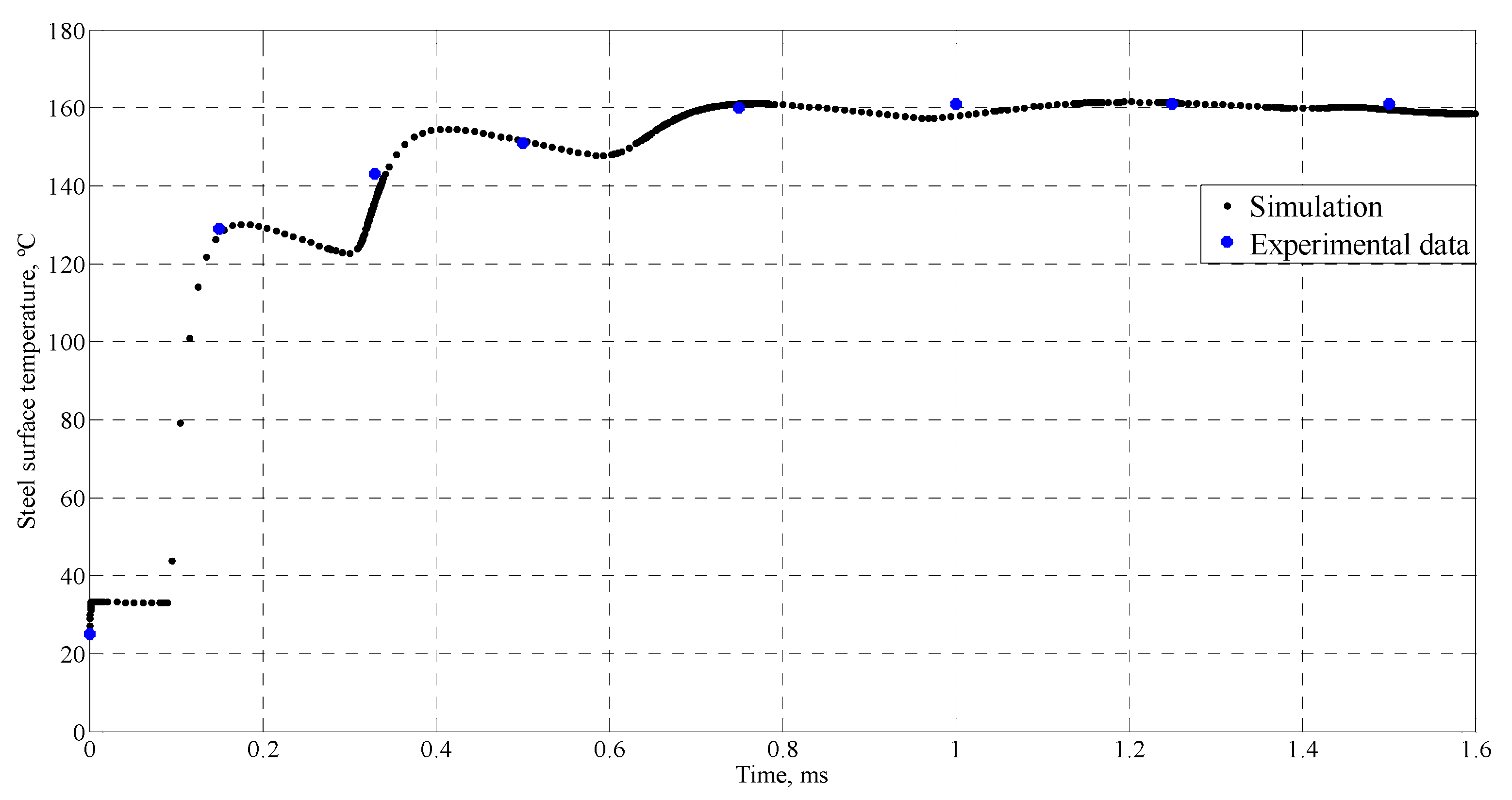
Figure 1. Section of substrate (dark grey) and splat (light grey).
Mathematics 08 01568 g001
Figure 2. Splat section from an impact in µm. (a) Slow impact (b) fast impact.
Mathematics 08 01568 g002
Figure 3. Cell used in the network model.
Mathematics 08 01568 g003
Figure 4. Network model for cell k.
Mathematics 08 01568 g004
Figure 5. Network model of the solidification equation.
Mathematics 08 01568 g005
Figure 6. Temperature evolution in the substrate cell 12211 without Rth and with Rth of 10−6 m2·K/W.
Mathematics 08 01568 g006
Figure 7. Temperature evolution of the splat cell 12322 without Rth and with Rth of 10−6 m2·K/W.
Mathematics 08 01568 g007
Figure 8. Comparison between experimental and simulated data for the steel temperature at the tin drop center.
Mathematics 08 01568 g008
Figure 9. Temperature evolution in the splat cell 12655 with and without thermal radiation.
Mathematics 08 01568 g009
Figure 10. Temperature evolution in the splat cells 12322, 12340 and 12358.
Mathematics 08 01568 g010
Figure 11. Temperature evolution in the splat cells 12655, 12673 and 12691.
Mathematics 08 01568 g011
Figure 12. Temperature evolution in the splat cells 12507, 12525 and 12543.
Mathematics 08 01568 g012
Figure 13. Temperature evolution in the steel cells 12211, 12229, 12247 and 12321.
Mathematics 08 01568 g013
Figure 14. Temperature evolution in the steel cells 1 and 5551.
Mathematics 08 01568 g014
Figure 15. Cooling rate (CR) evolution in the splat cells 12340, 12322 and 12655.
Mathematics 08 01568 g015
Figure 16. Temperature evolution in the splat cells 12322, 12340 and 12358 with preheating substrate.
Mathematics 08 01568 g016
Figure 17. Temperature evolution in the cells 12655, 12673 and 12691 with preheating substrate.
Mathematics 08 01568 g017
Figure 18. Temperature evolution in the centre of the splat surface for a fine and a rough mesh.
Mathematics 08 01568 g018
Table 1. Experimental data for steel temperature at the centre of tin drop [58].
Time (ms)Temperature (°C)
025
0.15129
0.33143
0.5151
0.75160
1161
1.25161
1.5161
Rth of 10−6 m2·K/W.

