1. Introduction
Water has vital importance for the survival of living beings. It is the basic element in terms of maintaining life in nature and human activities. The fact that 75% of the Earth’s surface is covered with water creates a perception that water scarcity would never be an issue to be discussed; more than 97% of this water is seawater, 2% is a mass of ice, and the large part of the remaining 1% is groundwater which is difficult to reach [
1]. Only a tiny fraction of the water that forms the large part of our planet we live consists of healthy drinkable water. Thankfully, this water is renewed by nature’s solar-powered water cycle. With the evaporation fueled by the sun’s energy, water vapor is carried to the atmosphere. Of this evaporation, 86% occurs from the sea and 14% from land [
1]. Even though an equal amount falls back to the Earth as rain, sleet, or snow, the distribution of water is more on continents than in oceans. With the transfer of water from the sea to land in this repeatable process, the renewable local drinking water resources occur. However, increasing population and air temperatures are effective factors in reducing drinking water availability per capita. The demand for drinking water will increase due to increasing population. A reduction in drinking water availability with increasing water demand, will equal an increase in stress on water supplies, as water supplies cannot be replenished quickly enough to meet demand. Moreover, agriculture already accounts for approximately 70% of the drinking water withdrawals in the world and is commonly seen as one of the main factors behind the growing global scarcity of freshwater [
2].
Although a lot of international agreements and declarations such as the International Convention on the Rights of the Child, [
3], the Human Rights Council Resolution, [
4], and the Water Framework Directive, [
5], stated the right to safe drinking water and sanitation is an internationally recognized human right, a great part of the world’s population cannot benefit from this right [
6].
Turkey, a country with land both in Asia and Europe and a population of approximately 81 million people, is exposed to dry seasons. European Environment Agency reported that Turkey will encounter moderate and high-level water scarcity in many areas [
7]. Thus, it is obvious that Turkey is a candidate country to experience problems with water scarceness. Considering that the population is predicted to be close to 100 million in 2030, [
8], it is crucial to take precautions to avoid water shortages and to produce better water policies. Hence, it is important for a country to both follow and also predict the tap water consumer ratios (TWCRs) particularly to take measures to decrease the negative effects of the reduction in tap water that could occur very soon.
Registered water use in a country is important to ensure planned and economical water use. Therefore, monitoring the TWCRs of watersheds and predictions of their near future values would make it easier to establish a basis for water-related precautions to form. In the literature, there are studies on water and its future predictions [
9,
10,
11,
12,
13]. Information on the assessment of sustainable water consumption perception, the evaluation of direct and indirect water consumption through the water footprint indicator, and the link between urban services and water uses are examined elsewhere [
14]. Water footprint is described as an indicator of water use in relation to human consumption [
15]. To incorporate the advances of life cycle assessment and water footprint analysis, an associated indicators set has been developed (see Reference [
16]). However, ignoring outliers which are points that differ from the bulk of the data or fit a different distribution could cause biases in the findings [
17].
This work aims to construct growth curve models (GCMs) to predict Turkey’s TWCRs. It is the ratio of the number of households using tap water in a particular region to the total number of households in that region. In this study, there are 26 grouped cities corresponding to 26 particular regions. Grouping of the cities is according to the watershed use of households. In the construction of the models, the non-robust ordinary least square estimator (OLS), which is employed in general, and robust least median square (LMS) and M estimators are used. This study demonstrates that detected outlying points differ according to which estimator is employed. Hence, every estimated model and hence the short-term predictions that are produced by the estimated model vary with respect to estimators. Thus, making better predictions for TWCRs to take convenient water policies depends on employing robust estimators that handle outliers very well during the parameter estimations of the GCMs. It is highlighted that the presence of outlying points has an undue impact on the model’s parameter estimations and future predictions.
The paper is organized as follows. In
Section 2 we introduce GCMs based on non-robust
OLS and, robust
LMS and
M estimators. To the best of our knowledge, this is the first time that robust
LMS and
M estimators are studied in this context. We show the differences in the outlying points, estimated GCMs, and hence the predictions by using the data originated in
Section 3. Here, the TWCRs of Turkey are estimated by considering that the straight-line growth model, in other words, the first-order GCM, of time could be fitted to data. In the estimation procedure, we use
OLS,
LMS, and
M estimators as mentioned above. As well as detection of outlying points, predictions to TWCRs of chosen years are obtained. Furthermore, to follow the estimations and predictions obtained from the estimated first-order GCMs based on
OLS, LMS, and
M estimators, separately, the curves are plotted on a single figure. Considering that the data could match more a third-order polynomial the progress is repeated for third-order GCMs.
2. GCMs Based on OLS, LMS, and M Estimators
The GCM usually expressed as
is the change in a growth that corresponds to the response variable
. This model indicates analytically how the parameters
and their standard errors
behave in a deterministic procedure for varying points of time [
18].
and
are the design matrices. Here,
used for grouped repeated measures is not taken into account since only the growth of Turkey’s TWCRs in watersheds on different time points is the subject to be researched. At this point, the vector of unknown parameters, the error, and the design matrix are denoted as
,
, and
, respectively. Each column of
is assumed to be distributed as
-variate normal with
the mean vector and
the unknown covariance matrix. Additionally,
is distributed as
where
is the expected value,
and
are the covariance matrices of
(
fixed and
) and
(
), respectively [
18]. The number of time points examined on each of
observations is denoted by
and
is the degree of the polynomial in time.
The
OLS estimator of
, which is defined as
, is obtained from
. The
is the expected value of
at time point 0 and called as the estimation of coefficient
. The
is the expected value of
when a one-unit change in time has occurred for observation
and called the estimation of coefficient
. In addition, the
OLS estimation of
, described as
, is based on
and is calculated from [
18].
Regarding the detection of outliers, the sum of squares of residuals of the
ith observation is calculated from
. Since
is chi-square distributed with
degrees of freedom, the calculated value of it is compared with the critical value determined from
, where
denotes the significance level. If the sum of squares of a suspicious observation is larger than the critical value, it would be appraised as an outlier [
19,
20]. The definition and explanations for
mentioned above are also valid for
LMS and
M estimators.
The estimation procedure of
and
with robust
LMS and
M estimators depends on the weighted least square (
WLS) estimator. Thus, the estimation procedure for
WLS is based on minimizing
, [
21]. The
WLS estimator of
, which is denoted as
, is computed from
and the estimation of the weighted covariance matrix is computed from
where
. The notation “
” denotes the trace. The elements of the diagonal weight matrix
that is used in Equation (3) and the calculation of
vary according to which estimator will be obtained. For instance, the
ith element,
, of the diagonal weight matrix,
, is defined as
when employing the
LMS estimator and
t is a value that ranges from 1 to
. Here,
denotes the number of
h-combinations from a given data set of
n elements and
h is calculated from
The notation
means rounding to a lower integer. Then, the
LMS estimators of
and
, defined as
and
, can be easily obtained by regarding the minimization problem of the objective function
where
[
19].
The
M estimator,
, is obtained by solving the objective function
where
. Here, the value of
is used for the initial point
. In Equation (8),
indicates a function which has a minimum at 0 for all
and
k shows the iteration number. In this instance, Tukey’s
function defined as
is used to compute
[
20]. In Equation (9),
means the derivative of
. The
ith diagonal element of the diagonal weight matrix
is obtained from:
Here, and is calculated as the value that provides , where is the expected value obtained from the chi-squared distribution with p degrees of freedom.
3. Application to the GCMs on Predictions of TWCRs in Turkey for Deciding Which Estimator Is the Best
3.1. The Dataset
Turkey consists of eighty-one cities. These cities are categorized into twenty-six groups according to which local watershed they benefit from [
8].
Table 1 summarizes TWCRs for each of them from 2001 to 2004 and at two-year intervals from 2006 to 2016.
In this research work, the response variable represents a matrix and the observed value of denoted by is the TWCR of group in the year , with and . The design matrix is employed in two ways since the data could specify a functional form of linear or a cubic growth. Firstly, it is a dimensional matrix where the first column consists of 1′s and the second column is the numbers 1 to 4 and 6, 8, 10, 12, 14, 16 used for the chosen years 2001 to 2004 and 2006, 2008, 2010, 2012, 2014, 2016, respectively. Hence, it is possible to preserve years as the unit of time. As it has been explained, does not affect the estimations. Thus, it is taken as an dimensional vector consisting of 1′s. With the benefit of this design, the parameters of GCMs denoted as and would be estimated. Three different methods including OLS, LMS, and M are used to reconstruct GCMs, separately. This makes it possible to show that the differences in the results of identified outlier observations vary regarding the methods.
In the second part of the study, the design matrix
where the first column consists of ones and the other columns consists of the numbers that correspond to the chosen years [
18], is employed. The reason for using the first, second, and third power of these numbers in the design matrix, respectively, is to build third-order GCMs. [
17]. Here,
is employed as defined previously in the construction of the first-order GCMs.
3.2. Detection of Outliers
The results of detecting outliers in the data, which consists of TWCRs in Turkey’s watersheds at different time points, and the parameter estimations of the GCMs according to methods mentioned above are summarized in
Table 2, when
. This table summarizes the findings that are observed for first- and third-order GCMs. Watershed number 9 has been identified as outlier with both non-robust and robust estimators. This is strong evidence that there is an outlier in the data. However, when applying robust
LMS and
M estimators, watersheds numbered 4, 19, 25, and 1, 5, 22, respectively, are detected as outlying points, besides the watershed numbered 9. Thus, it is safe to infer that the predictions obtained from the estimated GCM based on
OLS can be adversely affected by the undetected outliers. By definition,
LMS and
M estimators are more resistant to outliers compared to the
OLS estimator [
18,
19,
20]. Therefore, it is suggested to consider the predictions obtained from the estimated GCM based on these estimators.
3.3. Results
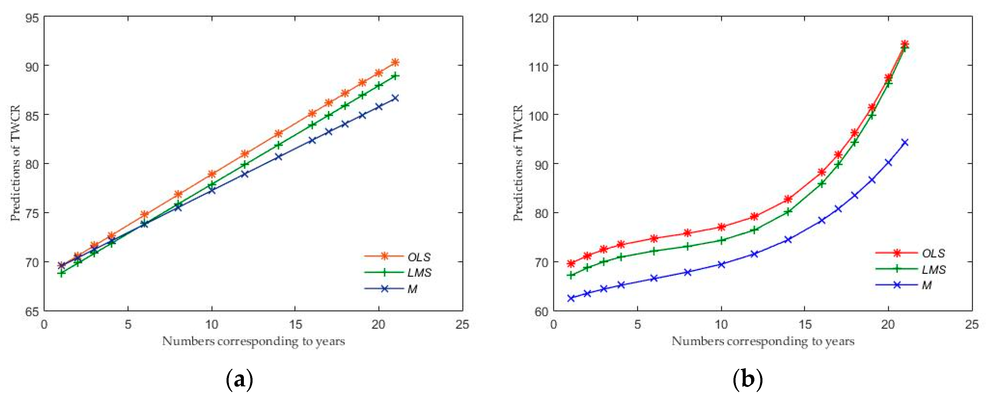
To show the differences in the estimated GCMs depended on
OLS, LMS, and
M estimators,
Figure 1a,b are plotted. The horizontal line denotes the numbers corresponding to years and the vertical line denotes the predictions of ratios. Regarding the estimated first-order GCMs in
Figure 1a, it is observed that the GCMs based on the
OLS,
LMS,
M estimators are different. The observed predictions from the
OLS appear to be larger when compared with the predictions from the
LMS and
M estimators. Knowing that the
OLS estimator is being influenced by the outlier points, it is better to evaluate the predictions obtained from
LMS and
M estimators due to their robustness to outlier points [
18,
19,
20]. Even, in general, the predictions of TWCRs obtained from the
OLS and
LMS estimators are higher than the predictions of TWCRs obtained from the
M estimator. The
M estimator is more resistant to outliers than the
OLS and
LMS estimators [
18,
19,
20]. Therefore, it is recommended to evaluate the results obtained from the
M estimator. For instance, the predictions for 2021 seem to be approximately 86%, 89%, and 90% in the case of using
M,
LMS, and
OLS estimators, respectively. Thus, it is highlighted that the outlying observations affect the results. The predictions of the ratios of watersheds at years 2017 to 2021 (corresponds to 17 to 21, respectively) could be seen from these graphs as well. The values of the predictions based on the three methods tend to increase over the years.
In addition, estimating and predicting procedures are repeated as the data could be more appropriate for a third-order GCM.
Figure 1b illustrates the estimated third-order GCMs after using
OLS,
LMS, and
M estimators and the predictions of TWCRs for watersheds in Turkey from 2017 to 2021 (corresponds to 17 to 21, respectively).
The differences between the estimated third-order polynomials can be seen clearly in this figure. Predictions on TWCRs of Turkey’s watersheds have risen steadily, particularly after 2015. Moreover, even the results for
M estimator are much lower than the results for
OLS and
LMS estimators. In addition, the predictions based on the
M estimator are observed below 100. Thus, predictions obtained from this estimator are said to be acceptable since the vertical line in
Figure 1b denotes the ratios. Consequently, it is proposed to consider the observed predictions from the
M estimator because of its robustness against outlying points.
4. Conclusions
GCMs, as statistical growth models for short-term predictions, are used for various studies. Based on tap water consumer data in Turkey recorded between the years 2001 and 2016, this study investigated the TWCRs of Turkey’s watersheds with first- and third-order GCMs for short-time predictions. To estimate the parameters of the models,
OLS, LMS, and
M estimators are used. Usage of both robust and non-robust estimators allowed us to remark on the differences in parameter estimates (
Table 2) and short-term predictions for TWCRs (
Figure 1). A legitimate clarification for these findings seems to be the existence of outliers in the data. The predictions obtained through the
M estimator are assumed to be the best, due to its robustness against outlier points [
18,
19,
20]. According to these predictions, the TWCRs for Turkey’s watersheds will constantly increase. Furthermore, a prediction based on the estimated third-order GCM for the year 2021 is expected to be approximately 5% more than in 2020. Hence, making short-term predictions with the robust
M estimator means a better view of the truth, which will lead us to produce better improvements on water policies.


