Article

Hybrid Annealing Krill Herd and Quantum-Behaved Particle Swarm Optimization

1
Department of Computer Science and Technology, Ocean University of China, Qingdao 266100, China
2
Institute of Algorithm and Big Data Analysis, Northeast Normal University, Changchun 130117, China
3
School of Computer Science and Information Technology, Northeast Normal University, Changchun 130117, China
4
Key Laboratory of Symbolic Computation and Knowledge Engineering of Ministry of Education, Jilin University, Changchun 130012, China
*
Author to whom correspondence should be addressed.
Mathematics 2020, 8(9), 1403; https://doi.org/10.3390/math8091403
Submission received: 27 July 2020 / Revised: 15 August 2020 / Accepted: 17 August 2020 / Published: 21 August 2020
(This article belongs to the Special Issue Evolutionary Computation 2020)

Abstract

:
The particle swarm optimization algorithm (PSO) is not good at dealing with discrete optimization problems, and for the krill herd algorithm (KH), the ability of local search is relatively poor. In this paper, we optimized PSO by quantum behavior and optimized KH by simulated annealing, so a new hybrid algorithm, named the annealing krill quantum particle swarm optimization (AKQPSO) algorithm, is proposed, and is based on the annealing krill herd algorithm (AKH) and quantum particle swarm optimization algorithm (QPSO). QPSO has better performance in exploitation and AKH has better performance in exploration, so AKQPSO proposed on this basis increases the diversity of population individuals, and shows better performance in both exploitation and exploration. In addition, the quantum behavior increased the diversity of the population, and the simulated annealing strategy made the algorithm avoid falling into the local optimal value, which made the algorithm obtain better performance. The test set used in this paper is a classic 100-Digit Challenge problem, which was proposed at 2019 IEEE Congress on Evolutionary Computation (CEC 2019), and AKQPSO has achieved better performance on benchmark problems.

1. Introduction

With the development of modern technology, artificial intelligence is becoming more and more important in society, and more and more mature, and can be used to deal with many problems that cannot be solved by traditional methods, such as wind energy decision system (WEDS) [1] and social cognitive radio network (SCRN) [2]. There are many kinds of classification methods; the simplest classification method is divided into the traditional method and modern intelligent method [3]. The traditional optimization algorithms generally deal with structured problems. The algorithms are deterministic and have only one global optimal solution. Meanwhile, the intelligent optimization algorithms generally deal with a more general description of the problems, which is heuristic, and have multiple extreme values. Intelligent optimization algorithms require certain strategies to prevent falling into the local optimum and try to find the global optimum, such as scheduling [4,5,6,7], image [8,9,10], feature selection [11,12,13] and detection [14,15], path planning [16,17], cyber-physical social system [18,19], texture discrimination [20], factor evaluation [21], saliency detection [22], classification [23,24], object extraction [25], gesture segmentation [26], economic load dispatch [27,28], shape design [29], big data and large-scale optimization [30,31], signal processing [32], multi-objective optimization [33,34], big data optimization [30,31], unit commitment [35], vehicle routing [36], knapsack problem [37,38,39], fault diagnosis [40,41,42], and test-sheet composition [43]. Because intelligent algorithms are not strictly dependent on the mathematical relationship, and because the problems that need to be solved are becoming more and more complex, intelligent algorithms are widely used to solve various complex optimization problems. As a result, the frequency of intelligent algorithms has exceeded that of traditional algorithms. At present, some main intelligent algorithms are widely used, such as genetic algorithm (GA) [44,45], particle swarm optimization algorithm (PSO) [46,47,48], krill herd (KH) [49,50,51,52,53,54], ant colony optimization algorithm (ACO) [55,56,57], differential evolution algorithm (DE) [58,59], adaptive island evolutionary algorithm (AIE) [60], and delayed start parallel evolutionary algorithm (DSPE) [61].
The swarm intelligence algorithms mainly come from the bionic idea, which is a set of methods summarized by referring to the laws of life and predatory behavior of animals in the biological world. A swarm intelligence algorithm is a kind of algorithm that works by studying the collective behavior of animals, and the most famous swarm intelligence algorithms are particle swarm optimization algorithm (PSO) [46] and ant colony optimization algorithm (ACO) [55]. An evolutionary algorithm is mainly a kind of method obtained by studying the process of biological genetic change, and these include genetic algorithm (GA) [44], genetic programming (GP) [62], evolutionary strategy (ES) [63,64], differential evolution (DE) [58] and other algorithms are based on genes. The krill herd (KH) [49] and quantum-behaved particle swarm optimization (QPSO) [65] algorithms mentioned in this paper belong to the swarm intelligence algorithm. The KH algorithm has the advantages of simplicity, flexibility, and high computational efficiency, and the QPSO algorithm has a relatively fast convergence speed, but when they are used to solve the 100-Digit Challenge problems, they do not do well. Owing to the poor local optimization ability of QPSO, it is easy to fall into the local optimal value, so it does not solve this problem well. In order to study an algorithm with very high accuracy, as well as to simultaneously optimize the exploitation and exploration and improve the accuracy of annealing krill quantum particle swarm optimization (AKQPSO), we studied the KH algorithm with strong exploitation and the QPSO algorithm with strong exploration. By combining their advantages, the new algorithm overcomes their original shortcomings and has a strong ability in exploration and exploitation. We combine the advantages of KH and QPSO, and optimize them, forming the annealing krill quantum particle swarm optimization (AKQPSO) algorithm. The new algorithm solved the 100-Digit Challenge better. Moreover, the study solved the problem of the poor accuracy of general algorithms, and exploitation and exploration cannot achieve the optimal at the same time.
In this paper, the 100-Digit Challenge problem is difficult to solve by traditional methods, and we can solve this problem better by using a swarm intelligence algorithm. In 2002, academician Nick Trefethen of Oxford University and the Society for Industrial and Applied Mathematics (SIAM) jointly developed the 100-Digit Challenge problem, which was proposed mainly to test high-precision computing [18]. The challenge consists of ten problems, each of which needs to be accurate to ten decimal places, with a total of 100 digits, so the problem is named the 100-Digit Challenge. However, traditional methods need a lot of computation to solve this challenge, and they cannot get good results, so we use swarm intelligence algorithm to solve these problems, and get satisfactory results.
The rest of paper is organized as follows. Most representative studies regarding the KH and QPSO algorithm are reviewed in Section 2, and these two algorithms are introduced in Section 3. The proposed algorithm is described in Section 4 and the experimental results of AKQPSO are presented in Section 5. Section 6 provides the main conclusions and highlights future work.

2. Related Work

In order to illustrate the hybrid method, we introduced KH and PSO algorithms. In the following, we will introduce the KH algorithm, PSO algorithm, and 100-Digit Challenge problem, respectively.

2.1. KH

At present, we have two kinds of optimizations for the KH algorithm [49]; one is to improve the KH algorithm itself, and the other is to improve the KH by other excellent operators or algorithms. Wang et al. [54] changed the parameters of the KH algorithm and improved the speed of global convergence through chaos theory. Then, in order to improve the performance, they [66] used harmony search to replace the physical diffusion, which greatly improved the performance and efficiency. These algorithms belong to the first category, which optimized the KH algorithm itself. The following are the second category, which optimized the algorithm with better strategies. Abualigah et al. [50] put forward a new algorithm, which combined harmony search algorithm with he KH algorithm to generate a new probability factor and improved exploration search ability, so as to get a better solution. Another algorithm is proposed by Abualigah et al. [67], which combined the objective function with the KH algorithm, and had better performance in solving the problem of text clustering. Niu et al. [68] sped up the exploration convergence and improved the efficiency by using the opposite learning strategy, using a sinusoidal graph to change the inertia weight, and modifying the search process according to the inertia weight and acceleration coefficient.

2.2. PSO

The PSO algorithm is one of the most famous swarm intelligence algorithms [47,69,70]. It was proposed in 1995, and it has the advantages of few parameters, a simple principle, and fast convergence. This algorithm has been widely used. For example, Sun et al. [71] used the agent model to assist the PSO algorithm to solve complex optimization problems. Through the combination of exploration and exploitation, they can better solve high-dimensional problems with limited resources. Similarly, for high-dimensional problems, Tran et al. [72] changed the fixed length of feature selection in the PSO algorithm, so that the particle swarm had a shorter length. This operation reduced the search space and gave shorter particles better performance. Thus, the overall efficiency of the PSO algorithm is improved, and it is also more suitable for high-dimensional problems. For the feature selection of the PSO algorithm, they [73] also optimized other methods. They improved the algorithm by discretizing the feature selection, and proved that the single variable discretization may reduce the performance of the feature selection stage, so they proposed a new discretization method, and got better performance. Zhang et al. [74] considered that there was no PSO algorithm that can work in noisy and noiseless environment at the same time, so they proposed the dual-environment PSO algorithm. This new algorithm is based on the top-k elite particles to search, which not only guaranteed the good performance in the noise environment, but also can be re-applied to the noise-free environment, so it filled a gap in the field of the PSO algorithm.

2.3. 100-Digit Challenge

The 100-Digit Challenge problem was originally proposed by SIAM [75], which is a test method for accuracy calculation, and has been studied by many experts. Many algorithms have been applied to this challenge, and some of them are hybrid algorithms that are used to challenge this problem. Epstein et al. [76] combined the genetic algorithm (GA) with differential evolution (DE) algorithm to search the genetic space and find the latest solution. The new algorithm improved the ability to find the right answer through the fitness-based opposition and tide mutation. Brest et al. [77] used the self-adaptive differential evolution (jDE) algorithm in the DE algorithm to solve this problem, and also got better results. Different from the above algorithms, Zhang et al. [78] proposed a new DE algorithm named collective information powered DE. This new algorithm proposed a restart mechanism through collective population information to improve the robustness.

3. KH and PSO

KH and PSO are very efficient algorithms in the field of swarm intelligence, and we will respectively introduce them in the following.

3.1. KH

In the process of predation, the predator will change the distribution of krill population, which will make them move rapidly, and then cause their distribution density to decrease and the distance between the predator and the food to become more and more far, which is the initial stage of KH. In this process, the distribution of krill population is determined by the following three situations: the influence of other krill individuals, behavior of getting food, and random diffusion. The KH algorithm can be described as follows:
d X i d t = N i + F i + D i
where Ni is the influence of other krill individuals, Fi is the behavior of getting food, and Di is the behavior of random diffusion; i = 1, 2, …, N, and N is the population size.
For the influence of other krill individuals, the motion Ni,new of krill i induced by other krill is defined as follows:
N i , n e w = N max α i + ω n N i , o l d
where Nmax represents the maximum induced velocity, Ni,old represents the previously induced movement, ωn represents the inertia weight and the value range is (0,1), and αi indicates that the individuali is affected by the induction direction of the surrounding neighbors.
The next behavior Fi is to get food, as follows:
F i = V f β i + ω f F i , o l d
where Vf is the maximum foraging speed, and its value is a constant, which is 0.02 (ms−1); ωf is the inertia weight of foraging movement, and its range is (0, 1); Fi,old is the previous foraging movement; and β i is the foraging direction.
The individual Di in the last behavior can be represented as follows:
D i = D max ( 1 I I max ) δ
where Dmax represents the maximum random diffusion speed; δ represents the direction of random diffusion; and I and Imax represent the current number and the maximum number of iterations, respectively. From above process, we can get the krill update process of the KH algorithm as follows:
X i ( t + Δ t ) = X i ( t ) + Δ t d X i d t
Δ t = C t j = 1 N V ( U B j L B j )
where Δt is the time interval related to the specific application; NV is the dimension of the decision variable; step factor Ct is a constant between 0 and 2; and UBj and LBj are the upper and lower bounds of corresponding variable j (j = 1, 2, …, NV), respectively.
The process of the KH algorithm (Algorithm 1) is as follows.
Algorithm 1. KH [49]
1. Begin
2. Step 1: Initialization. Initialize the generation counter G, the population P, Vf, Dmax, and Nmax.
3. Step 2: Fitness calculation. Calculate fitness for each krill according to its initial position.
4. Step 3: WhileG < MaxGeneration do
   5. Sort the population according to their fitness.
   6. for i = 1:N (all krill) do
   7. Perform the following motion calculation.
     8. Motion induced by other individuals
     9. Foraging motion
     10. Physical diffusion
   11. Implement the genetic operators.
   12. Update the krill position in the search space.
   13. Calculate fitness for each krill according to its new position
14. end for i
15. G = G + 1.
16. Step 4: end while.
17. End.

3.2. PSO

In the PSO algorithm, each individual is called a “particle”, and each particle will find a potential optimal solution at each iteration. Assuming that the size of the population is N, each particle i (i = 1, 2, …, N) in the population has its own initial position Xi (Xi = xi1, xi2, …, xid) and initial velocity Vi (Vi = vi1, vi2, …, vid), and they will search for the optimal solution in D-dimensional space according to their own individual extremum pbest and global extremum gbest. Individual extremum is the current best point found by each particle in the search space, and global extremum is the current best point found by the whole particle group in the search space. During the search process, the updating formula of particle’s relevant state parameters is as follows:
v i t + 1 = η v i t + c 1 r a n d 1 ( ) · ( p b e s t t x i t ) + c 2 r a n d 2 ( ) · ( g b e s t t x i t )
x i t + 1 = x i t + v i t
η = η s t a r t ( η s t a r t η e n d ) t T
where η is the inertia weight that determines the specific gravity of the particle to the current velocity. If the η is large, the particle has a strong exploration ability and can span a longer distance to find the global optimal solution, but it may cause the particle to oscillate back and forth before and after the optimal solution. If the η is small, it means that particles have better ability to find the optimal solution locally, but they can easily to fall into the local optimization solution.
The flow of the standard PSO algorithm (Algorithm 2) is given below, where bup and blo represent the upper and lower bounds of the problem domain, respectively, and D represents the dimension of the solution space.
Algorithm 2. PSO [46]
Begin
  Step 1: Initialization.
    1. Initial position: the initial position of each particle obeys uniform distribution, that is X i ~ U ( b u p , b l o ) .
    2. Initialize its own optimal solution and the overall optimal solution: the initial position is its own optimal solution pi = xi, and then calculating the corresponding value of each particle according to the defined utility function f, and find the global optimal solution gbest.
    3. Initial speed: the speed also obeys the uniform distribution.
  Step 2: Update.
  According to Equations (7) and (8), the velocity and position of particles are updated, and the current fitness of particles is calculated according to the utility function f of the problem. If it is better than its own historical optimal solution, it will update its own historical optimal solution pbest, otherwise it will not update. If the particle’s own optimal solution pbest is better than the global optimal solution g, then the global optimal solution g is updated, otherwise it is not updated.
  Step 3: Determine whether to terminate:
  Determine whether the best solution meets the termination conditions, if yes, stop.
  Otherwise, return to Step 2.
End.
As shown in Equations (7) and (8), during each iteration, the particles update the direction and speed of the next flight based on their own and group experience. The main characteristics of the PSO algorithm are as follows:
  • Particles have memory. Each iteration of particles will transfer the optimal solution of the population to each other, and update the database of all particles. If the particles deviate, the direction and velocity can be corrected by self-cognition and group-cognition.
  • PSO algorithm has fewer parameters, so it is easy to adjust, and the structure is simple, so it is easy to implement.
  • The operation is simple, and it only searches for the optimal solution in the solution space according to the flight of particles.

4. AKQPSO

The AKQPSO algorithm is a mixed metaheuristic algorithm, which combines the advantages of annealing krill herd (AKH) and QPSO [79]. AKH solves the disadvantage that KH cannot escape from the local optimal solution. At the same time, the efficiency of KH algorithm is improved by the simulated annealing strategy. Quantum behaved PSO (QPSO) is a new algorithm proposed by Sun et al. [79] in 2004. By introducing the quantum behavior and combining it with the idea of simulated annealing, the search ability of AKQPSO is greatly improved, and the new algorithm has better performance. The principle of QPSO is shown below.
Quantum computing is a new computing mode, which follows the laws of quantum mechanics and regulates the quantum information unit. In quantum space, when the aggregation state property is satisfied, particles can search in the whole feasible solution space, thus greatly improving the exploration search ability of QPSO. According to the analysis theory of particle convergence trajectory, if every particle can converge to its local attraction point Pi = (pi1, pi2 …, pid), then the algorithm has the possibility of convergence. The particle position update expression of the standard QPSO algorithm is as follows:
x i j t + 1 = p i j t ± α · | C i j t x i j t | · ln [ 1 / u i j t ] , u i j t ~ U ( 0 , 1 )
where α is the only parameter that needs to be adjusted in the algorithm, called the compression-expansion factor, which is used to control the convergence rate of particles. During the iterative process, the calculation method of individual and global optimal position is the same as that of the PSO algorithm, and the biggest difference is that the QPSO algorithm removes the speed information.
First of all, we initialize the whole population, and all the individuals in the population are randomly generated. After initialization, we divide the population into two subpopulations according to the ratio of 3:7, which is discussed in Section 5.2. The population with the proportion of 3/10 is optimized by the improved KH algorithm, which is called subpopulation-AKH, and the population with the proportion of 7/10 is optimized by the QPSO algorithm, which is called subpopulation-QPSO. The two subpopulations will be re-integrated into a population after iterative optimization. If the optimization result of the new population meets the output conditions, then the result can be output. However, if it does not meet the output conditions, then it can be re-divided according to the proportion of 3:7, and repeat the above process until the results meet the termination conditions. In the process of decentralized and re-fusion of this population, the location information of individuals is shared, so it will greatly improve the efficiency of fusion search and get the best results faster. In the process of the AKQPSO algorithm, we also optimized the KH algorithm by the idea of simulated annealing, named annealing KH (AKH), so we used QPSO and simulated annealing strategy to guarantee the algorithm to escape from the local optimal value. The framework of AKQPSO is shown in Figure 1 and the process of the AKQPSO algorithm (Algorithm 3) is as follows.
Algorithm 3 AKQPSO
Initialization:
  N random individuals were generated.
  Set initialization parameters of AKH and QPSO.
Evaluation:
  Evaluate all individuals based on location.
Partition:
  The whole population was divided into subpopulation-AKH and subpopulation-QPSO.
AKH process:
  Subpopulation-AKH individuals were optimized by AKH.
  Update through these three actions of the influence of other krill individuals, behavior of getting food and random diffusion.
  The simulated annealing strategy is used to deal with the above behaviors.
  Update the individual position according to the above behavior.
QPSO process:
  Subpopulation-QPSO individuals were optimized by QPSO.
  Update the particle’s local best point Pi and global best point Pbest.
  Update the position x i j t + 1 by Equation (10).
Combination:
  The population optimized by AKH and QPSO was reconstituted into a new population.
Finding the best solution:
  The fitness of all individuals was calculated, and the best solution was found in the newly-combined population.
Determine whether to terminate:
  Determine whether the best solution meets the termination conditions, if yes, stop.
  Otherwise, return to step Evaluation.

5. Simulation Results

The 100-Digit Challenge problem comes from CEC 2019 and can be found through the website http://www.ntu.edu.sg/home/EPNSugan/index_files/CEC2019. This challenge includes 10 problems, which are 10 functions in our data. The goal is to calculate the accuracy of the function to 10 digits without a time limit. The proposed algorithm was written in MATLAB R2016a and was run in the following conditions: Intel(R) Core(TM) i5-8100 CPU 3.60 GHz, which possesses 8G of RAM on Windows 10. Table 1 shows the basic parameters of the 100-Digit Challenge. The 10 test problems are the definition of minimization and some other definitions are as follows:
Min f ( x ) , x = [ x 1 , x 2 , , x D ] T
where D is the dimension, the global optimal value of the shift is randomly distributed in (−80, 80), and all testing problems are scalable.

5.1. The Comparison of AKQPSO and Other Algorithms

In this paper, we compared the AKQPSO algorithm with the following eight state-of-the-art algorithms.
  • By improving krill migration operator, biogeography-based KH (BBKH) [51] was proposed.
  • By adding a new hybrid differential evolution operator, the efficiency of the updating process is improved, and differential evolution KH (DEKH) [80] was proposed.
  • By quantum behavior to optimize KH, quantum-behaved KH (QKH) [65] was proposed.
  • By adding the stud selection and crossover operator, the efficiency was improved and stud krill herd (SKH) [81] was proposed.
  • By adding chaos map to optimize cuckoo search (CS), the chaotic CS (CCS) [82] was proposed.
  • By adding variable neighborhood (VN) search to bat algorithm (BA), VNBA [83] was proposed.
  • By discussing physical biogeography and its mathematics, biogeography-based optimization (BBO) [84] was proposed.
  • Genetic algorithm (GA) [45] is basic algorithm of evolutionary computing.
Table 2 is the common parameter setting of these algorithms. We set the population size (N) to 50; after 7500 iterations (max_gen) and 100 independent runs (max_run), all algorithm experiments are carried out under the condition that the basic parameters are consistent.
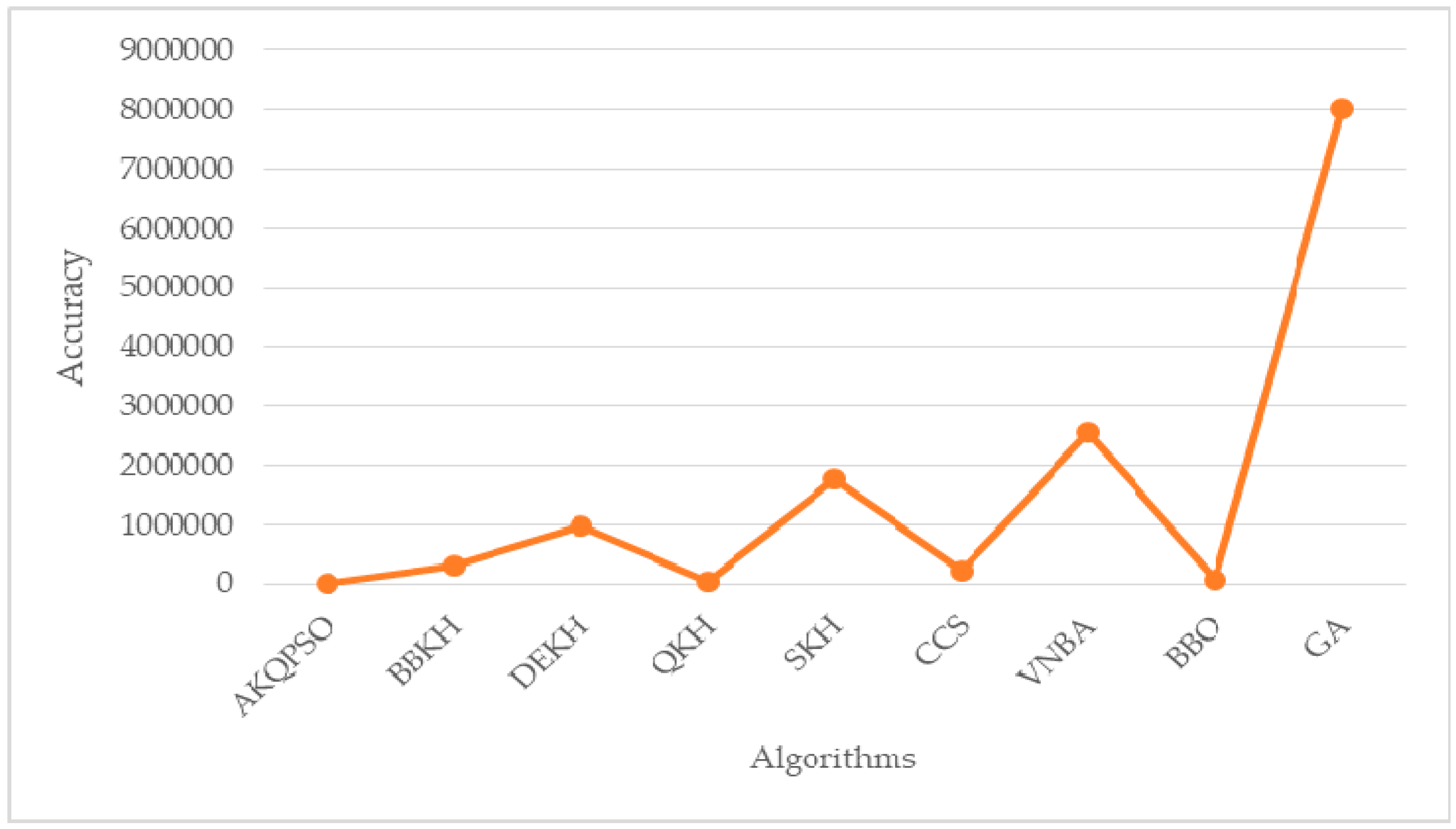
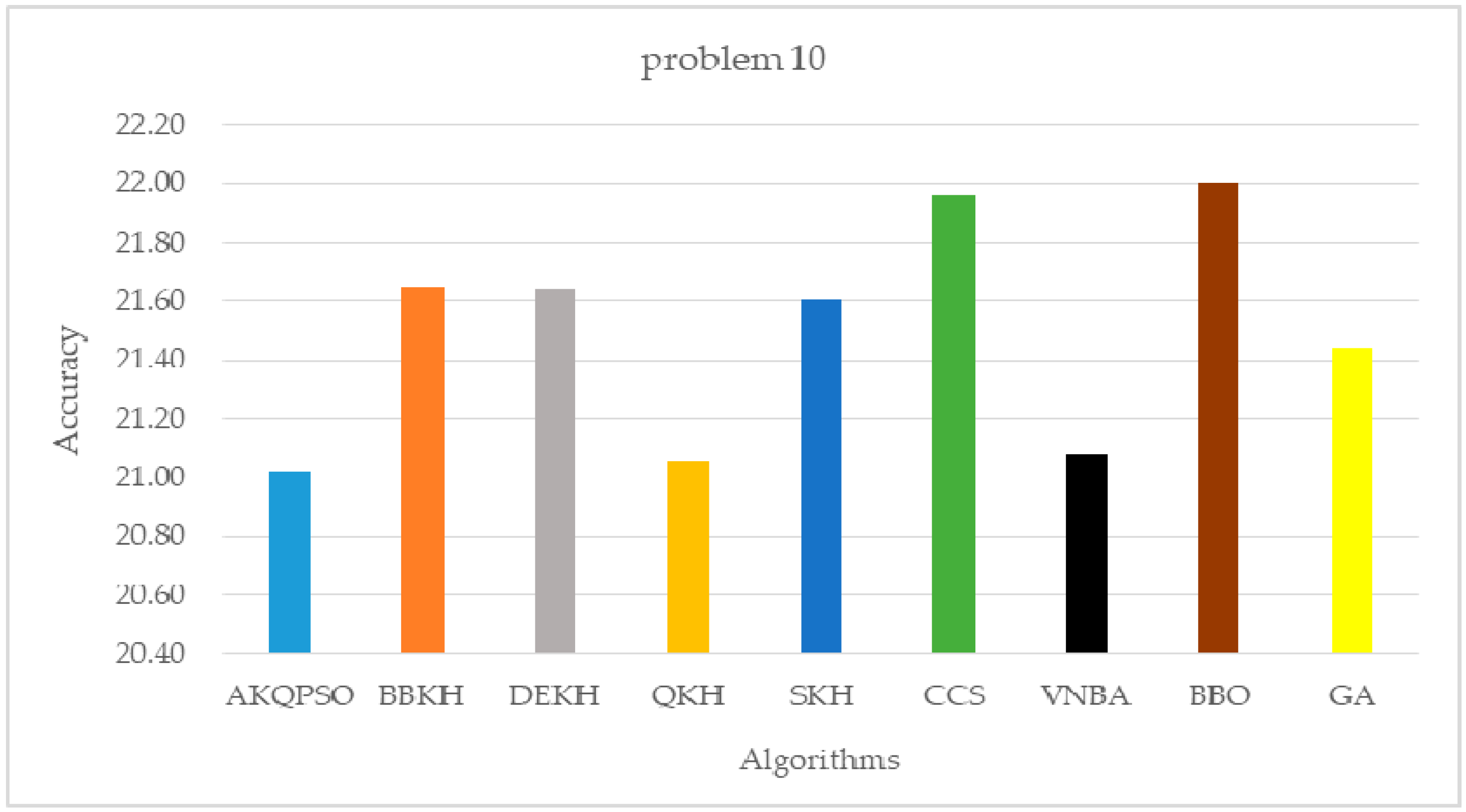
Table 3 shows the optimization results of AKQPSO and eight other algorithms for ten of the 100-Digits Challenge, with the best value in bold. From the experimental results, we can see that the optimal values of the ten problems are all calculated by the AKQPSO algorithm. AKQPSO is the best algorithm among these algorithms, and the result is the best in every problem, but QKH is not the second in every problem, so we can know that our algorithm improvement is very effective. Through Figure 2, we can clearly conclude that the performance of AKQPSO is the best in general, followed by QKH, and the performance of GA is the worst. In general, we rank the algorithms as follows: AKQPSO > QKH > CCS > BBKH > DEKH > SKH > VNBA > GA.
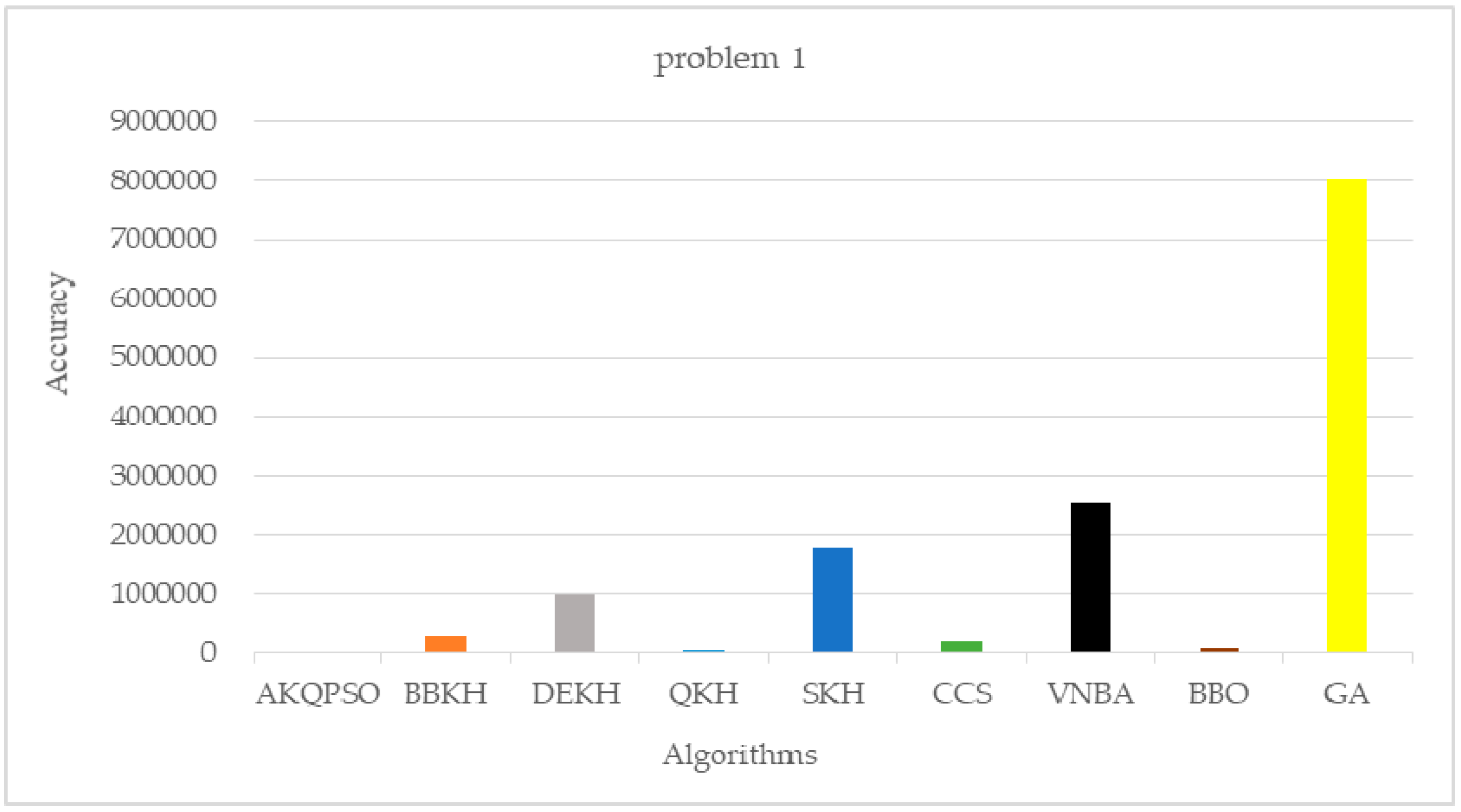
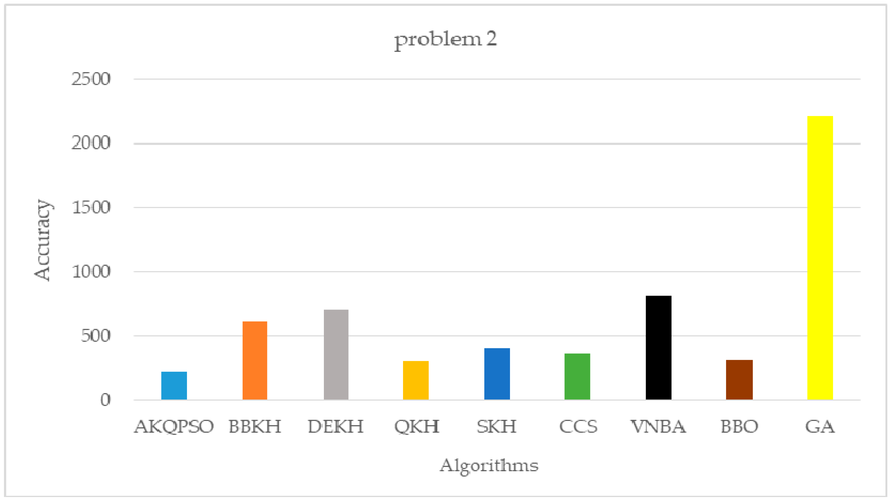
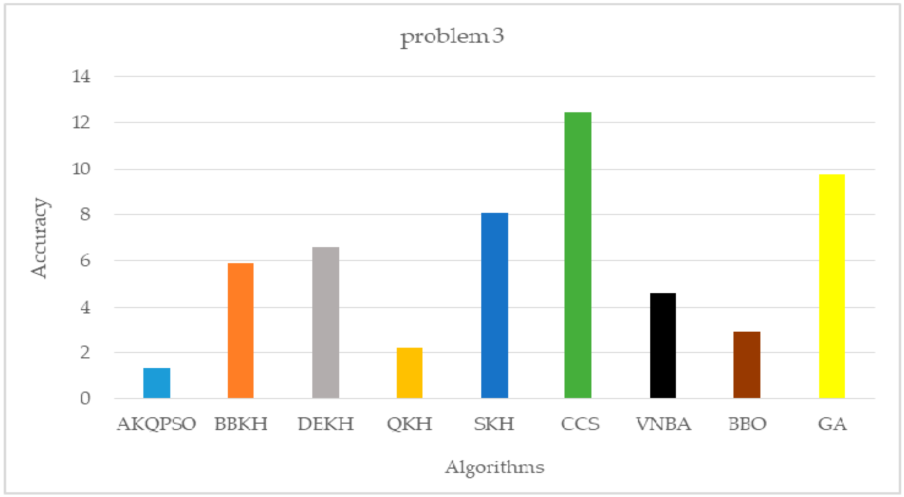
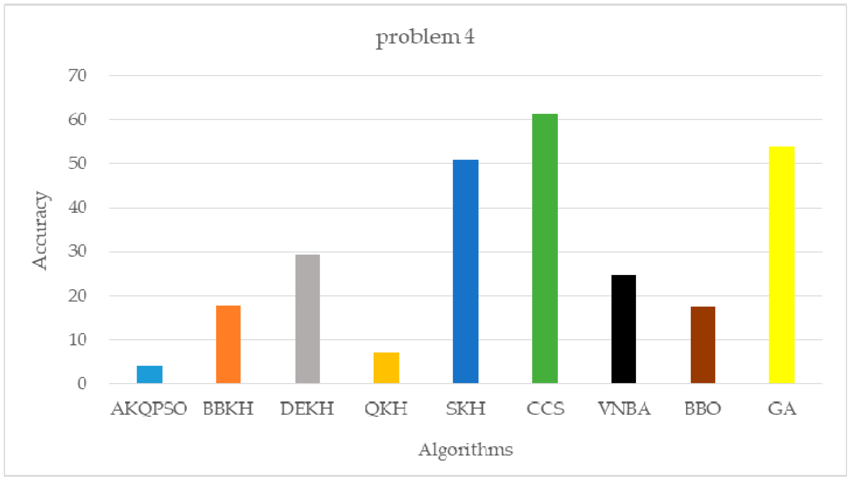
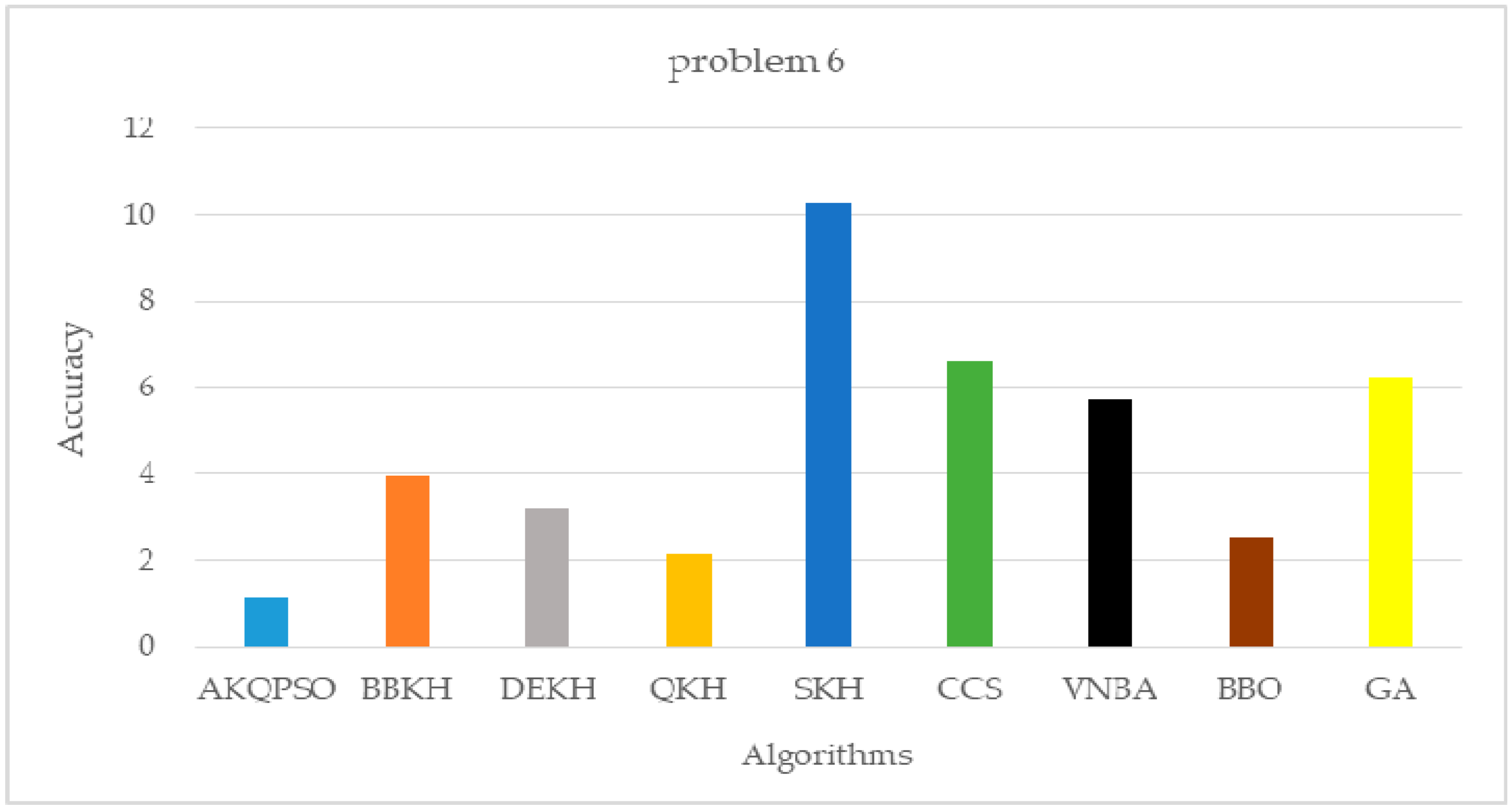
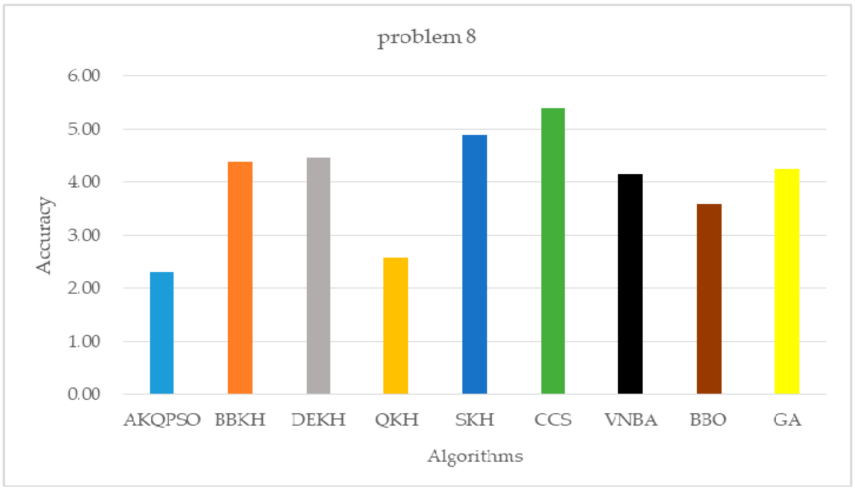
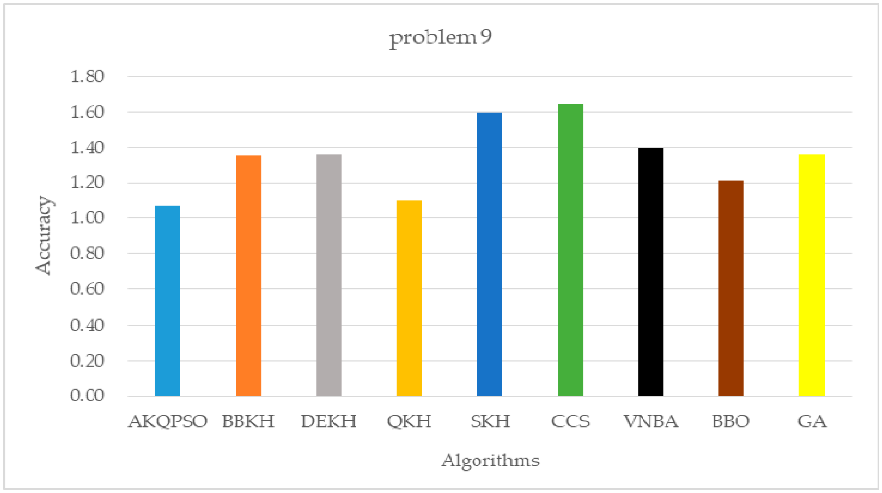
Figure 3, Figure 4, Figure 5, Figure 6, Figure 7, Figure 8, Figure 9, Figure 10, Figure 11 and Figure 12 show the results of the nine algorithms on each problem, and the experimental results show that AKQPSO algorithm has obvious advantages over other algorithms. From these column charts, we can see that the fluctuation of problem 1 is the largest. In problem 1, the results of the GA algorithm with the worst performance are 735 times different from those of AKQPSO algorithm with the best performance, which can be said to be very different. Because the 100-Digits Challenge problem is used to test the computational accuracy, we can know that the computational accuracy of AKQPSO algorithm is the highest among the nine algorithms. In Figure 3, because the results of AKQPSO, QKH, and BBO are so different from those of GA, the columns of these algorithms are almost invisible, so they are not obvious in the same chart. However, in fact, the improvement of AKQPSO compared with QKH and BBO is significant.
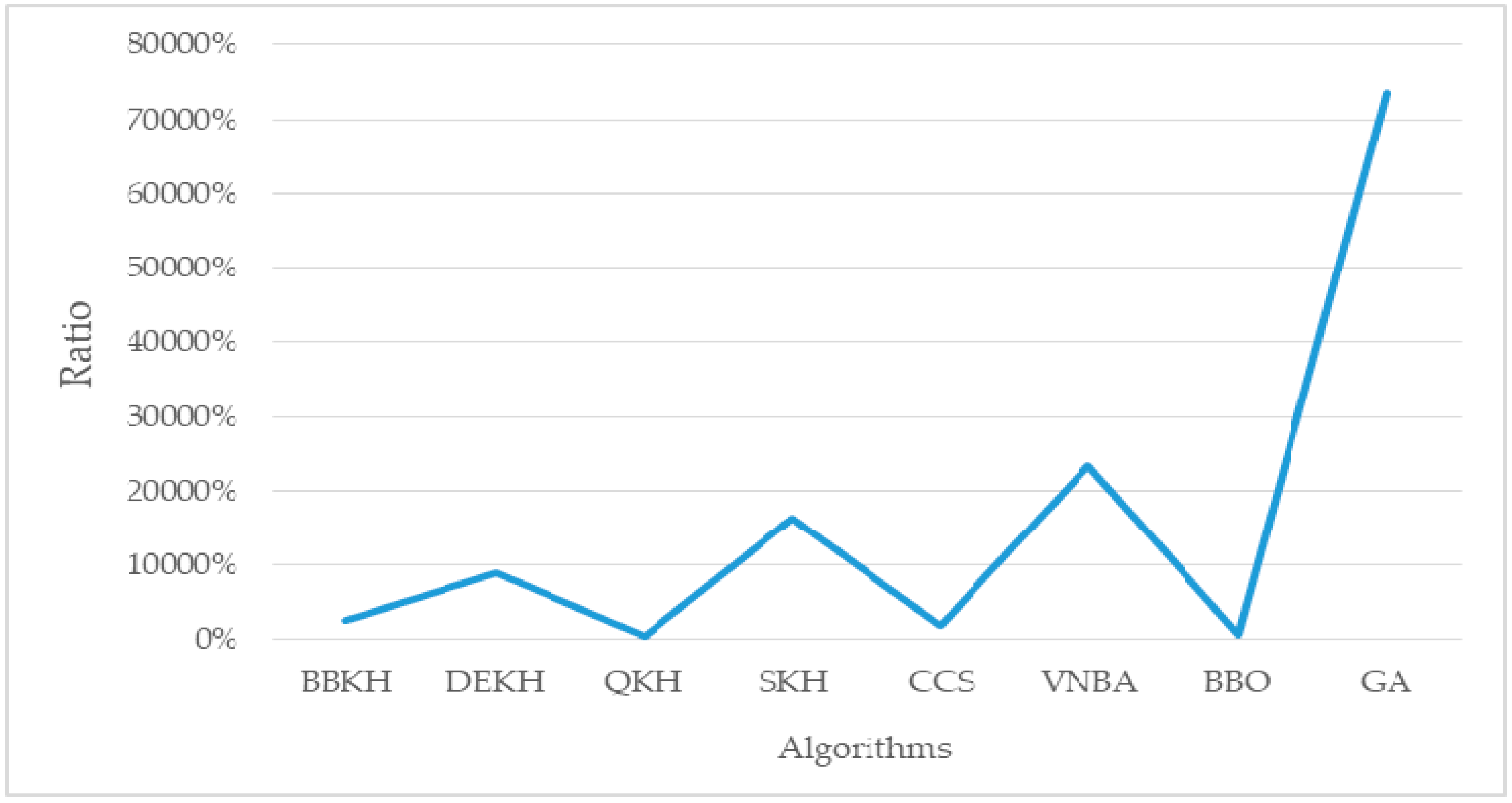
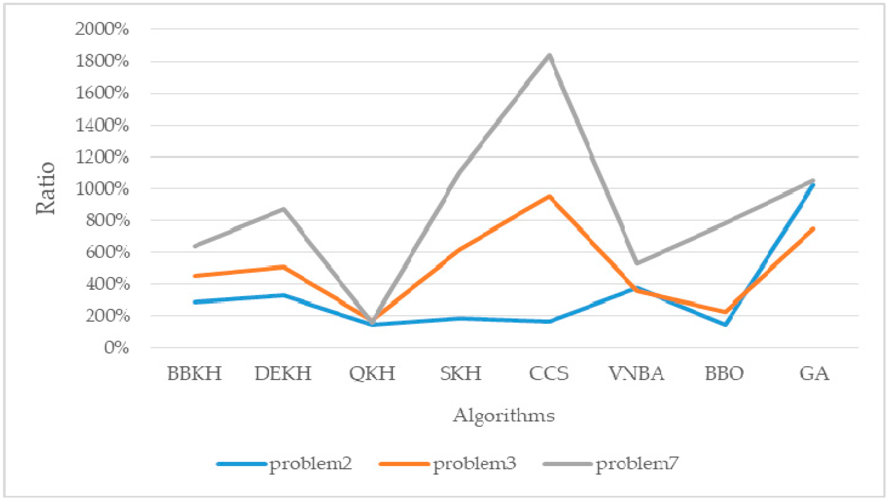
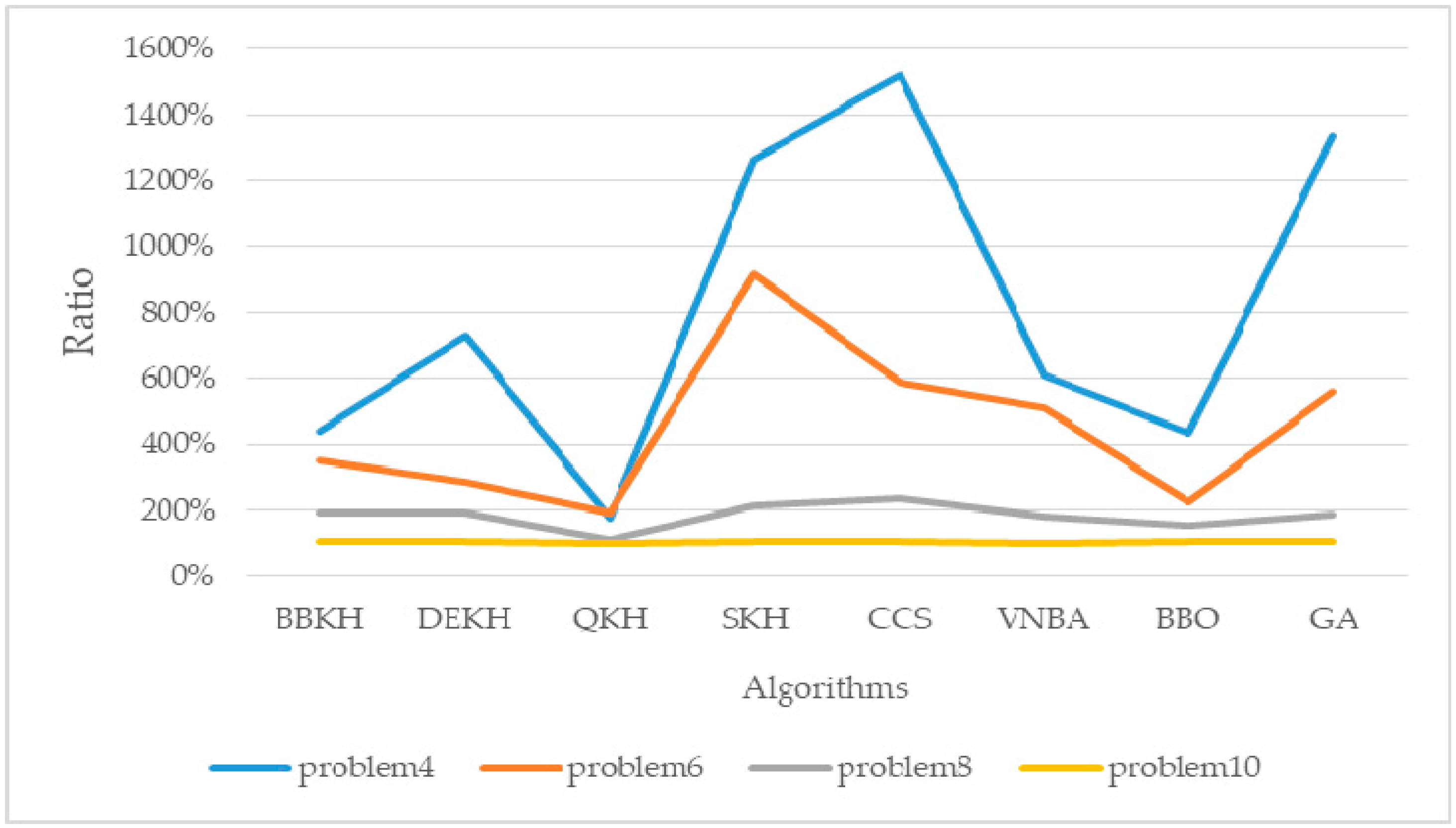
Among these ten problems, we divide the problems into four groups according to the ability of these problems to test the computational accuracy of AKQPSO. Some groups have a strong ability to test, so it is more obvious which algorithm is better. The first group: problem 1. According to the computational accuracy, the results displayed in this group are quite different. The second group: problems 2, 3, and 7. This group has higher requirements for the accuracy, so it is difficult to calculate the best value of the function. The third group: problems 4, 6, 8, and 10. This group has a slightly lower requirement for the computational accuracy, so the results of various algorithms are very close, but it is difficult to achieve the best results. The fourth group: problems 5 and 9. This group has the lowest requirements for the computational accuracy, so many algorithms can be very close to the optimal result 1.0000000000.
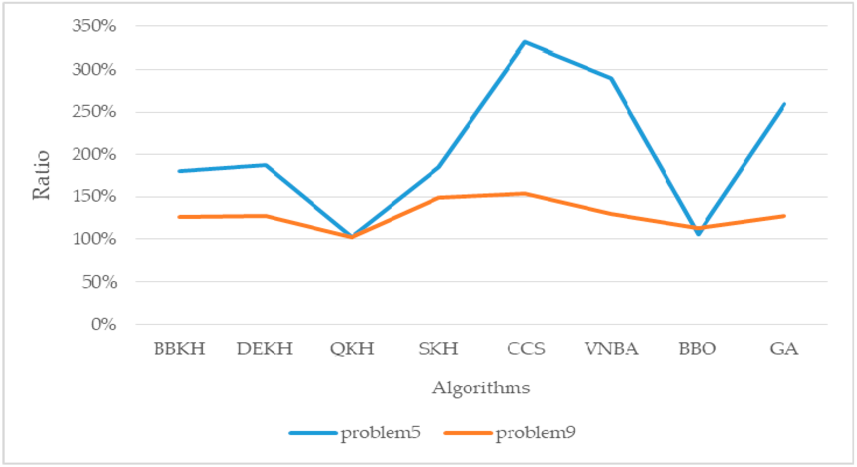
Figure 13, Figure 14, Figure 15 and Figure 16 show the advantage of AKQPSO over other algorithms in each group of the 100-Digits Challenge problem. Although the accuracy of GA is the worst when ranking from the whole, and in the first of the four groups, it is also the GA. In the other three groups, however, the algorithm with the worst accuracy is CCS algorithm, so in terms of grouping comparison, CCS algorithm is the worst. In addition, the accuracy of AKQPSO algorithm is still the best among the four groups, which has not changed. From the above analysis, AKQPSO is the best in all aspects, and the computational accuracy of this algorithm is also the highest.

5.2. Evaluation Parameter λ

In Section 4, after the initialization of the population, AKQPSO algorithm divided the population into two subpopulations: AKH and QPSO. We set the parameter λ, which represents the proportion of the two subpopulations. In the experiment, λ = 0.1, 0.2, …, 0.9. For example, if λ = 0.1, this means that the ratio of subpopulation-AKH/subpopulation-QPSO is 1:9, and other numbers mean the same thing. After a lot of experiments, the optimal parameter value is λ = 0.3. All the above experiments are based on the results obtained using λ = 0.3, and the following part will introduce the experiments on λ = 0.3. The parameters of this part of experiments are still the same as Table 2 to ensure that all experiments are tested under the same conditions.
Table 4 shows the experimental results of 10 problems that are calculated by different λ in the AKQPSO algorithm in the 100-Digit Challenge. Bold font indicates the best value. From Table 4, we can see that, in the case of λ = 0.3, eight of the ten problems can get the best value. In the remaining two problems, even if λ = 0.3 does not reach the best value, its result is the second among the nine values, and it is very close to the best value. Therefore, when λ = 0.3, the performance of AKQPSO can reach the best.
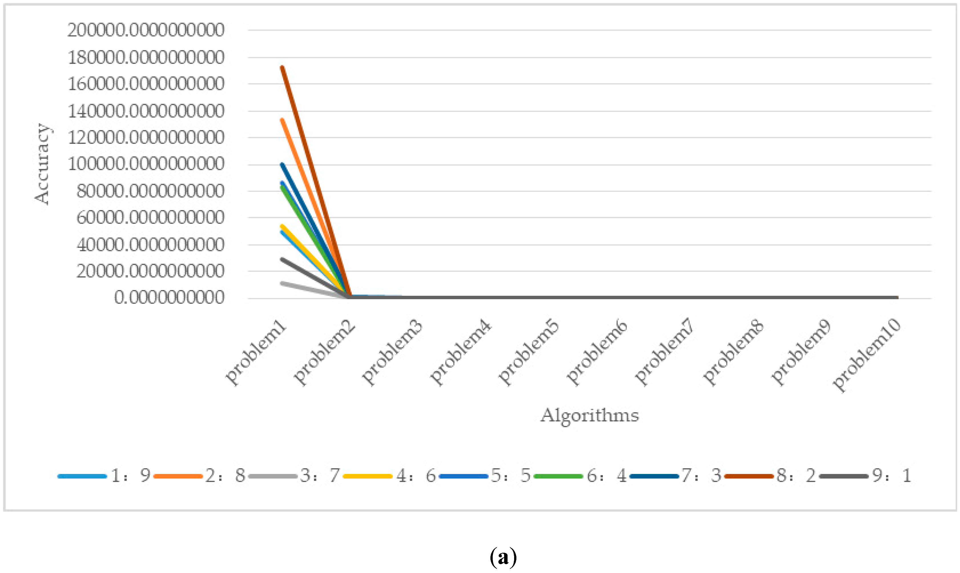
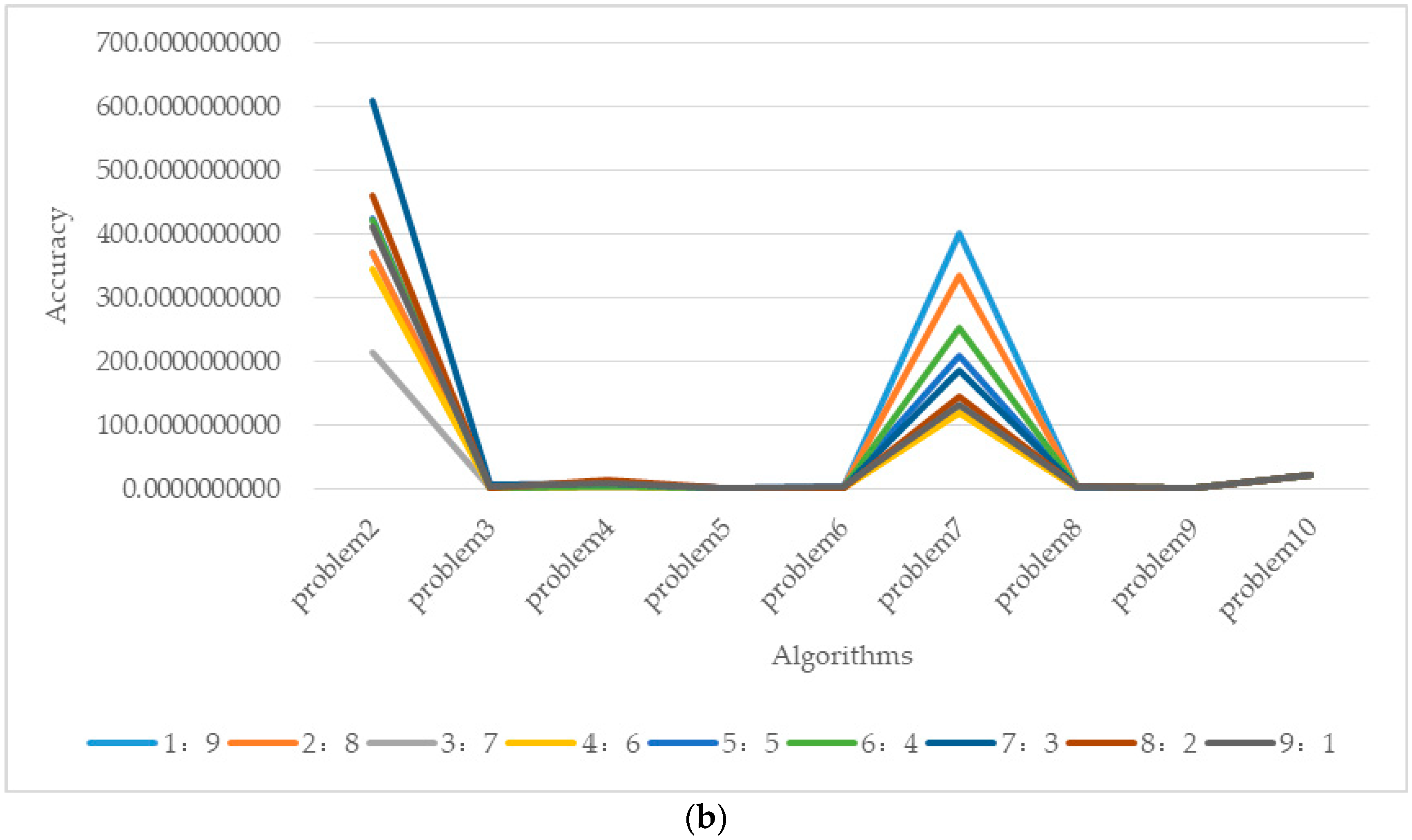
As can be seen from Figure 17a, the fluctuation range of the result of problem 1 is the largest. As problems 1–10 are in the same chart, and the fluctuation of problem 1 is much larger than that of other problems, the fluctuation range of problems 2–10 is not obvious in Figure 17a. In order to compare problems 2–10 more clearly, we used Figure 17b to show the fluctuation of other problems 2–10. Through Figure 17b, we can see that the fluctuation of problems 2 and 7 are also obvious. Therefore, among these ten problems, problems 1, 2, and 7 are the three problems with the largest fluctuation. Among these ten problems, the fluctuation of problem 7 is different from that of the other nine problems. With the increasing proportion of AKH and QPSO, the result of problem 7 tends to be better. For other problems, however, with the increasing proportion of AKH and QPSO, their results tend to be worse, which is the opposite of problem 7.
From the results of Section 5.1 and Section 5.2, problems 1, 2, and 7 belong to the first and the second of the four groups, respectively, and they are also the two groups with the highest requirements for the computational accuracy of AKQPSO. Therefore, the adjustment of subpopulation has a very direct effect on the accuracy of AKQPSO.

5.3. Complexity Analysis of AKQPSO

The main computing overhead of AKQPSO associated with Step “Partition” of the AKQPSO algorithm in Section 4. The following is a detailed analysis of the single computational complexity of Step “Partition” and other step in AKQPSO. N is the number of individuals in the population.
  • Step “Partition”: This step accounts for the main computational overhead, so we focus on this step.
    • Step “AKH process”: The computational complexity of this step mainly includes “Subpopulation-AKH individuals were optimized by AKH”, “Update through these three actions of the influence of other krill individuals, behavior of getting food and random diffusion”, “The simulated annealing strategy is used to deal with the above behaviors”, and “Update the individual position according to the above behavior”, and their complexities are O(N), O(N2), O(N), and O(N), respectively.
    • Step “QPSO process”: The computational complexity of this step mainly includes “Subpopulation-QPSO individuals were optimized by QPSO”, “Update the particle’s local best point Pi and global best point Pbest”, and “Update the position x i j t + 1 by Equation (10)”, and their complexities are all O(N).
  • Other step.
    • The computational complexity of Step “Initialization”, Step “Evaluation”, Step “Combination”, and Step “Finding the best solution” are all O(N).
Therefore, in one generation AKQPSO, the worst-case complexity is O(N2).

6. Conclusions

In this paper, aiming at the disadvantage of poor local search ability of KH algorithm, we optimized it by simulated annealing strategy and QPSO algorithm, and proposed a new algorithm: AKQPSO. This algorithm was compared with eight other excellent algorithms, and the computational accuracy of AKQPSO was tested by the 100-Digit Challenge problem. As predicted before the experiment, the computational accuracy of AKQPSO algorithm is the highest among these algorithms. Moreover, we also adjusted the parameters of AKQPSO through experiments to further improve the computational accuracy. By calculating the accuracy of the 100-Digit Challenge problem, our experiment provided a new method to study the accuracy of the algorithm, and the paper provided a very high accuracy algorithm. However, the research of this paper still has some limitations. The accuracy of the algorithm in 100-Digit Challenge problem is very high, but it is unclear whether AKQPSO still has high accuracy in general problems.
In the future, we can focus on other aspects. Firstly, besides the simulated annealing strategy and QPSO algorithm, we could look for other metaheuristic algorithms [85] that can be used to improve the search ability of KH and carry out in-depth research such as bat algorithm (BA) [86,87], biogeography-based optimization (BBO) [84,88], cuckoo search (CS) [82,89,90,91,92], earthworm optimization algorithm (EWA) [93], elephant herding optimization (EHO) [94,95], moth search (MS) algorithm [96], firefly algorithm (FA) [97], artificial bee colony (ABC) [98,99,100], harmony search (HS) [101], monarch butterfly optimization (MBO) [102,103], and genetic programming (GP) [104], as well as more recent research. Secondly, for the parameters in the algorithm, besides the proportion of subpopulation, we can also study the influence of other parameters on the computational accuracy of AKQPSO. Thirdly, now we just use two kinds of algorithms to make them cooperate and optimize in a relatively simple way, and we can also study how to make them cooperate more efficiently through other methods. Finally, although the 100-Digit Challenge is a classical problem, it is still less used for testing computational accuracy of algorithms, and there is still a large development space in this area.

Author Contributions

Conceptualization, C.-L.W. and G.-G.W.; methodology, C.-L.W.; software, G.-G.W.; validation, C.-L.W.; formal analysis, G.-G.W.; investigation, C.-L.W.; resources, G.-G.W.; data curation, C.-L.W.; writing—original draft preparation, C.-L.W.; writing—review and editing, C.-L.W.; visualization, C.-L.W.; supervision, G.-G.W.; project administration, G.-G.W.; funding acquisition, G.-G.W. All authors have read and agreed to the published version of the manuscript.

Funding

This research was funded by National Natural Science Foundation of China, grant number U1706218, 41576011, 41706010 and 61503165.

Conflicts of Interest

The authors declare no conflict of interest.

References

  1. Zhao, X.; Wang, C.; Su, J.; Wang, J. Research and application based on the swarm intelligence algorithm and artificial intelligence for wind farm decision system. Renew. Energy 2019, 134, 681–697. [Google Scholar] [CrossRef]
  2. Anandakumar, H.; Umamaheswari, K. A bio-inspired swarm intelligence technique for social aware cognitive radio handovers. Comput. Electr. Eng. 2018, 71, 925–937. [Google Scholar] [CrossRef]
  3. Shang, K.; Ishibuchi, H. A New Hypervolume-based Evolutionary Algorithm for Many-objective Optimization. IEEE Trans. Evol. Comput. 2020, 1. [Google Scholar] [CrossRef]
  4. Sang, H.-Y.; Pan, Q.-K.; Duan, P.-Y.; Li, J.-Q. An effective discrete invasive weed optimization algorithm for lot-streaming flowshop scheduling problems. J. Intell. Manuf. 2015, 29, 1337–1349. [Google Scholar] [CrossRef]
  5. Sang, H.-Y.; Pan, Q.-K.; Li, J.-Q.; Wang, P.; Han, Y.-Y.; Gao, K.-Z.; Duan, P. Effective invasive weed optimization algorithms for distributed assembly permutation flowshop problem with total flowtime criterion. Swarm Evol. Comput. 2019, 44, 64–73. [Google Scholar] [CrossRef]
  6. Pan, Q.-K.; Sang, H.-Y.; Duan, J.-H.; Gao, L. An improved fruit fly optimization algorithm for continuous function optimization problems. Knowl. Based Syst. 2014, 62, 69–83. [Google Scholar] [CrossRef]
  7. Gao, D.; Wang, G.-G.; Pedrycz, W. Solving Fuzzy Job-shop Scheduling Problem Using DE Algorithm Improved by a Selection Mechanism. IEEE Trans. Fuzzy Syst. 2020, 1. [Google Scholar] [CrossRef]
  8. Li, M.; Xiao, D.; Zhang, Y.; Nan, H. Reversible data hiding in encrypted images using cross division and additive homomorphism. Signal Process. Image Commun. 2015, 39, 234–248. [Google Scholar] [CrossRef]
  9. Li, M.; Guo, Y.; Huang, J.; Li, Y. Cryptanalysis of a chaotic image encryption scheme based on permutation-diffusion structure. Signal Process. Image Commun. 2018, 62, 164–172. [Google Scholar] [CrossRef]
  10. Fan, H.; Li, M.; Liu, N.; Zhang, E. Cryptanalysis of a colour image encryption using chaotic APFM nonlinear adaptive filter. Signal Process. 2018, 143, 28–41. [Google Scholar] [CrossRef]
  11. Zhang, Y.; Gong, D.-W.; Hu, Y.; Zhang, W. Feature selection algorithm based on bare bones particle swarm optimization. Neurocomputing 2015, 148, 150–157. [Google Scholar] [CrossRef]
  12. Zhang, Y.; Song, X.-F.; Gong, D.-W. A return-cost-based binary firefly algorithm for feature selection. Inf. Sci. 2017, 418, 561–574. [Google Scholar] [CrossRef]
  13. Mao, W.; He, J.; Tang, J.; Li, Y. Predicting remaining useful life of rolling bearings based on deep feature representation and long short-term memory neural network. Adv. Mech. Eng. 2018, 10, 10. [Google Scholar] [CrossRef]
  14. Jian, M.; Lam, K.M.; Dong, J. Facial-feature detection and localization based on a hierarchical scheme. Inf. Sci. 2014, 262, 1–14. [Google Scholar] [CrossRef]
  15. Fan, L.; Xu, S.; Liu, D.; Ru, Y. Semi-Supervised Community Detection Based on Distance Dynamics. IEEE Access 2018, 6, 37261–37271. [Google Scholar] [CrossRef]
  16. Wang, G.; Chu, H.E.; Mirjalili, S. Three-dimensional path planning for UCAV using an improved bat algorithm. Aerosp. Sci. Technol. 2016, 49, 231–238. [Google Scholar] [CrossRef]
  17. Wang, G.; Guo, L.; Duan, H.; Liu, L.; Wang, H.; Shao, M. Path Planning for Uninhabited Combat Aerial Vehicle Using Hybrid Meta-Heuristic DE/BBO Algorithm. Adv. Sci. Eng. Med. 2012, 4, 550–564. [Google Scholar] [CrossRef]
  18. Wang, G.; Cai, X.; Cui, Z.; Min, G.; Chen, J. High Performance Computing for Cyber Physical Social Systems by Using Evolutionary Multi-Objective Optimization Algorithm. IEEE Trans. Emerg. Top. Comput. 2017, 8, 1. [Google Scholar] [CrossRef]
  19. Cui, Z.; Sun, B.; Wang, G.; Xue, Y.; Chen, J. A novel oriented cuckoo search algorithm to improve DV-Hop performance for cyber-physical systems. J. Parallel Distrib. Comput. 2017, 103, 42–52. [Google Scholar] [CrossRef]
  20. Jian, M.; Lam, K.M.; Dong, J. Illumination-insensitive texture discrimination based on illumination compensation and enhancement. Inf. Sci. 2014, 269, 60–72. [Google Scholar] [CrossRef]
  21. Wang, G.-G.; Guo, L.; Duan, H.; Liu, L.; Wang, H. The model and algorithm for the target threat assessment based on elman_adaboost strong predictor. Acta Electron. Sin. 2012, 40, 901–906. [Google Scholar]
  22. Jian, M.; Lam, K.M.; Dong, J.; Shen, L. Visual-Patch-Attention-Aware Saliency Detection. IEEE Trans. Cybern. 2014, 45, 1575–1586. [Google Scholar] [CrossRef] [PubMed]
  23. Wang, G.; Lu, M.; Dong, Y.-Q.; Zhao, X.-J. Self-adaptive extreme learning machine. Neural Comput. Appl. 2015, 27, 291–303. [Google Scholar] [CrossRef]
  24. Mao, W.; Zheng, Y.; Mu, X.; Zhao, J. Uncertainty evaluation and model selection of extreme learning machine based on Riemannian metric. Neural Comput. Appl. 2013, 24, 1613–1625. [Google Scholar] [CrossRef]
  25. Liu, G.; Zou, J. Level set evolution with sparsity constraint for object extraction. IET Image Process. 2018, 12, 1413–1422. [Google Scholar] [CrossRef]
  26. Liu, K.; Gong, D.; Meng, F.; Chen, H.; Wang, G. Gesture segmentation based on a two-phase estimation of distribution algorithm. Inf. Sci. 2017, 88–105. [Google Scholar] [CrossRef] [Green Version]
  27. Parouha, R.P.; Das, K.N. Economic load dispatch using memory based differential evolution. Int. J. Bio-Inspired Comput. 2018, 11, 159–170. [Google Scholar] [CrossRef]
  28. Rizk-Allah, R.M.; El-Sehiemy, R.A.; Wang, G. A novel parallel hurricane optimization algorithm for secure emission/economic load dispatch solution. Appl. Soft Comput. 2018, 63, 206–222. [Google Scholar] [CrossRef]
  29. Rizk-Allah, R.M.; El-Sehiemy, R.A.; Deb, S.; Wang, G. A novel fruit fly framework for multi-objective shape design of tubular linear synchronous motor. J. Supercomput. 2017, 73, 1235–1256. [Google Scholar] [CrossRef]
  30. Yi, J.-H.; Xing, L.; Wang, G.; Dong, J.; Vasilakos, A.V.; Alavi, A.H.; Wang, L. Behavior of crossover operators in NSGA-III for large-scale optimization problems. Inf. Sci. 2020, 509, 470–487. [Google Scholar] [CrossRef]
  31. Yi, J.-H.; Deb, S.; Dong, J.; Alavi, A.H.; Wang, G. An improved NSGA-III algorithm with adaptive mutation operator for Big Data optimization problems. Future Gener. Comput. Syst. 2018, 88, 571–585. [Google Scholar] [CrossRef]
  32. Liu, G.; Deng, M. Parametric active contour based on sparse decomposition for multi-objects extraction. Signal Process. 2018, 148, 314–321. [Google Scholar] [CrossRef]
  33. Sun, J.; Miao, Z.; Gong, D.; Zeng, X.-J.; Li, J.; Wang, G.-G. Interval multi-objective optimization with memetic algorithms. IEEE Trans. Cybern. 2020, 50, 3444–3457. [Google Scholar] [CrossRef] [PubMed]
  34. Zhang, Y.; Wang, G.; Li, K.; Yeh, W.-C.; Jian, M.; Dong, J. Enhancing MOEA/D with information feedback models for large-scale many-objective optimization. Inf. Sci. 2020, 522, 1–16. [Google Scholar] [CrossRef]
  35. Srikanth, K.; Panwar, L.K.; Panigrahi, B.; Herrera-Viedma, E.; Sangaiah, A.K.; Wang, G. Meta-heuristic framework: Quantum inspired binary grey wolf optimizer for unit commitment problem. Comput. Electr. Eng. 2018, 70, 243–260. [Google Scholar] [CrossRef]
  36. Chen, S.; Chen, R.; Wang, G.; Gao, J.; Sangaiah, A.K. An adaptive large neighborhood search heuristic for dynamic vehicle routing problems. Comput. Electr. Eng. 2018, 67, 596–607. [Google Scholar] [CrossRef]
  37. Feng, Y.; Wang, G.-G. Binary moth search algorithm for discounted {0–1} knapsack problem. IEEE Access 2018, 6, 10708–10719. [Google Scholar] [CrossRef]
  38. Feng, Y.; Wang, G.; Wang, L. Solving randomized time-varying knapsack problems by a novel global firefly algorithm. Eng. Comput. 2018, 34, 621–635. [Google Scholar] [CrossRef]
  39. Abdel-Basst, M.; Zhou, Y. An elite opposition-flower pollination algorithm for a 0–1 knapsack problem. Int. J. Bio-Inspired Comput. 2018, 11, 46–53. [Google Scholar] [CrossRef]
  40. Yi, J.-H.; Wang, J.; Wang, G. Improved probabilistic neural networks with self-adaptive strategies for transformer fault diagnosis problem. Adv. Mech. Eng. 2016, 8, 1–13. [Google Scholar] [CrossRef] [Green Version]
  41. Mao, W.; He, J.; Li, Y.; Yan, Y. Bearing fault diagnosis with auto-encoder extreme learning machine: A comparative study. Proc. Inst. Mech. Eng. Part C J. Mech. Eng. Sci. 2016, 231, 1560–1578. [Google Scholar] [CrossRef]
  42. Mao, W.; Feng, W.; Liang, X. A novel deep output kernel learning method for bearing fault structural diagnosis. Mech. Syst. Signal Process. 2019, 117, 293–318. [Google Scholar] [CrossRef]
  43. Duan, H.; Zhao, W.; Wang, G.; Feng, X. Test-Sheet Composition Using Analytic Hierarchy Process and Hybrid Metaheuristic Algorithm TS/BBO. Math. Probl. Eng. 2012, 2012, 1–22. [Google Scholar] [CrossRef]
  44. Goldberg, D.E. Genetic algorithms in search. In Optimization, and Machine Learning; Addison-Wesley: Reading, MA, USA, 1989. [Google Scholar]
  45. Mistry, K.; Zhang, L.; Neoh, S.C.; Lim, C.P.; Fielding, B. A Micro-GA Embedded PSO Feature Selection Approach to Intelligent Facial Emotion Recognition. IEEE Trans. Cybern. 2017, 47, 1496–1509. [Google Scholar] [CrossRef] [PubMed] [Green Version]
  46. Kennedy, J.; Eberhart, R. Particle swarm optimization. In Proceedings of the IEEE International Conference on Neural Networks, Perth, Australia, 27 November–1 December 1995; pp. 1942–1948. [Google Scholar]
  47. Song, X.-F.; Zhang, Y.; Guo, Y.-N.; Sun, X.-Y.; Wang, Y.-L. Variable-size Cooperative Coevolutionary Particle Swarm Optimization for Feature Selection on High-dimensional Data. IEEE Trans. Evol. Comput. 2020, 1. [Google Scholar] [CrossRef]
  48. Sun, Y.; Jiao, L.; Deng, X.; Wang, R. Dynamic network structured immune particle swarm optimisation with small-world topology. Int. J. Bio-Inspired Comput. 2017, 9, 93–105. [Google Scholar] [CrossRef]
  49. Gandomi, A.H.; Alavi, A.H. Krill herd: A new bio-inspired optimization algorithm. Commun. Nonlinear Sci. Numer. Simul. 2012, 17, 4831–4845. [Google Scholar] [CrossRef]
  50. Abualigah, L.M.; Khader, A.T.; Hanandeh, E.S.; Gandomi, A.H. A novel hybridization strategy for krill herd algorithm applied to clustering techniques. Appl. Soft Comput. 2017, 60, 423–435. [Google Scholar] [CrossRef]
  51. Wang, G.; Gandomi, A.H.; Alavi, A.H. An effective krill herd algorithm with migration operator in biogeography-based optimization. Appl. Math. Model. 2014, 38, 2454–2462. [Google Scholar] [CrossRef]
  52. Wang, G.-G.; Gandomi, A.H.; Alavi, A.H.; Deb, S. A Multi-Stage Krill Herd Algorithm for Global Numerical Optimization. Int. J. Artif. Intell. Tools 2016, 25, 1550030. [Google Scholar] [CrossRef]
  53. Wang, G.; Gandomi, A.H.; Alavi, A.H.; Gong, D. A comprehensive review of krill herd algorithm: Variants, hybrids and applications. Artif. Intell. Rev. 2019, 51, 119–148. [Google Scholar] [CrossRef]
  54. Wang, G.; Guo, L.; Gandomi, A.H.; Hao, G.-S.; Wang, H. Chaotic Krill Herd algorithm. Inf. Sci. 2014, 274, 17–34. [Google Scholar] [CrossRef]
  55. Dorigo, M.; Maniezzo, V.; Colorni, A. Ant system: Optimization by a colony of cooperating agents. IEEE Trans. Syst. Man. Cybern. Part B Cybern. 1996, 26, 29–41. [Google Scholar] [CrossRef] [Green Version]
  56. Zheng, F.; Zecchin, A.C.; Newman, J.P.; Maier, H.R.; Dandy, G.C. An Adaptive Convergence-Trajectory Controlled Ant Colony Optimization Algorithm With Application to Water Distribution System Design Problems. IEEE Trans. Evol. Comput. 2017, 21, 773–791. [Google Scholar] [CrossRef]
  57. Dorigo, M.; Stutzle, T. Ant Colony Optimization; MIT Press: Cambridge, UK, 2004. [Google Scholar]
  58. Storn, R.; Price, K. Differential evolution—A simple and efficient heuristic for global optimization over continuous spaces. J. Glob. Optim. 1997, 11, 341–359. [Google Scholar] [CrossRef]
  59. Gao, S.; Yu, Y.; Wang, Y.; Wang, J.; Cheng, J.; Zhou, M. Chaotic Local Search-Based Differential Evolution Algorithms for Optimization. IEEE Trans. Syst. Man Cybern. Syst. 2019, 1–14. [Google Scholar] [CrossRef]
  60. Dulebenets, M.A. An Adaptive Island Evolutionary Algorithm for the berth scheduling problem. Memetic Comput. 2020, 12, 51–72. [Google Scholar] [CrossRef]
  61. Dulebenets, M.A. A Delayed Start Parallel Evolutionary Algorithm for just-in-time truck scheduling at a cross-docking facility. Int. J. Prod. Econ. 2019, 212, 236–258. [Google Scholar] [CrossRef]
  62. Agapitos, A.; Loughran, R.; Nicolau, M.; Lucas, S.; OrNeill, M.; Brabazon, A. A Survey of Statistical Machine Learning Elements in Genetic Programming. IEEE Trans. Evol. Comput. 2019, 23, 1029–1048. [Google Scholar] [CrossRef]
  63. Back, T. Evolutionary Algorithms in Theory and Practice: Evolution Strategies, Evolutionary Programming, Genetic Algorithms; Oxford University Press: Oxford, UK, 1996. [Google Scholar]
  64. Kashan, A.H.; Keshmiry, M.; Dahooie, J.H.; Abbasi-Pooya, A. A simple yet effective grouping evolutionary strategy (GES) algorithm for scheduling parallel machines. Neural Comput. Appl. 2016, 30, 1925–1938. [Google Scholar] [CrossRef]
  65. Wang, G.; Gandomi, A.H.; Alavi, A.H.; Deb, S. A hybrid method based on krill herd and quantum-behaved particle swarm optimization. Neural Comput. Appl. 2015, 27, 989–1006. [Google Scholar] [CrossRef]
  66. Wang, G.; Guo, L.; Wang, H.; Duan, H.; Liu, L.; Li, J. Incorporating mutation scheme into krill herd algorithm for global numerical optimization. Neural Comput. Appl. 2012, 24, 853–871. [Google Scholar] [CrossRef]
  67. Abualigah, L.M.; Khader, A.T.; Hanandeh, E.S. A combination of objective functions and hybrid Krill herd algorithm for text document clustering analysis. Eng. Appl. Artif. Intell. 2018, 73, 111–125. [Google Scholar] [CrossRef]
  68. Niu, P.; Chen, K.; Ma, Y.; Li, X.; Liu, A.; Li, G. Model turbine heat rate by fast learning network with tuning based on ameliorated krill herd algorithm. Knowl. Based Syst. 2017, 118, 80–92. [Google Scholar] [CrossRef]
  69. Slowik, A.; Kwasnicka, H. Nature Inspired Methods and Their Industry Applications—Swarm Intelligence Algorithms. IEEE Trans. Ind. Inform. 2018, 14, 1004–1015. [Google Scholar] [CrossRef]
  70. Brezočnik, L.; Fister, J.I.; Podgorelec, V. Swarm Intelligence Algorithms for Feature Selection: A Review. Appl. Sci. 2018, 8, 1521. [Google Scholar] [CrossRef] [Green Version]
  71. Sun, C.; Jin, Y.; Cheng, R.; Ding, J.; Zeng, J. Surrogate-Assisted Cooperative Swarm Optimization of High-Dimensional Expensive Problems. IEEE Trans. Evol. Comput. 2017, 21, 644–660. [Google Scholar] [CrossRef] [Green Version]
  72. Tran, B.N.; Xue, B.; Zhang, M. Variable-Length Particle Swarm Optimization for Feature Selection on High-Dimensional Classification. IEEE Trans. Evol. Comput. 2019, 23, 473–487. [Google Scholar] [CrossRef]
  73. Tran, B.N.; Xue, B.; Zhang, M. A New Representation in PSO for Discretization-Based Feature Selection. IEEE Trans. Cybern. 2018, 48, 1733–1746. [Google Scholar] [CrossRef]
  74. Zhang, J.; Zhu, X.; Wang, Y.; Zhou, M. Dual-Environmental Particle Swarm Optimizer in Noisy and Noise-Free Environments. IEEE Trans. Cybern. 2019, 49, 2011–2021. [Google Scholar] [CrossRef]
  75. Bornemann, F.; Laurie, D.; Wagon, S.; Waldvogel, J. The siam 100-digit challenge: A study in high-accuracy numerical computing. SIAM Rev. 2005, 1, 47. [Google Scholar]
  76. Epstein, A.; Ergezer, M.; Marshall, I.; Shue, W. Gade with fitness-based opposition and tidal mutation for solving ieee cec2019 100-digit challenge. In Proceedings of the 2019 IEEE Congress on Evolutionary Computation (CEC), Wellington, New Zealand, 10–13 June 2019; pp. 395–402. [Google Scholar]
  77. Brest, J.; Maučec, M.S.; Bošković, B. The 100-digit challenge: Algorithm jde100. In Proceedings of the 2019 IEEE Congress on Evolutionary Computation (CEC), Wellington, New Zealand, 10–13 June 2019; pp. 19–26. [Google Scholar]
  78. Zhang, S.X.; Chan, W.S.; Tang, K.S.; Zheng, S.Y. Restart based collective information powered differential evolution for solving the 100-digit challenge on single objective numerical optimization. In Proceedings of the 2019 IEEE Congress on Evolutionary Computation (CEC), Wellington, New Zealand, 10–13 June 2019; pp. 14–18. [Google Scholar]
  79. Jun, S.; Bin, F.; Wenbo, X. Particle swarm optimization with particles having quantum behavior. In Proceedings of the 2004 Congress on Evolutionary Computation, Portland, OR, USA, 19–23 June 2004; Volume 321, pp. 325–331. [Google Scholar]
  80. Wang, G.; Gandomi, A.H.; Alavi, A.H.; Hao, G.-S. Hybrid krill herd algorithm with differential evolution for global numerical optimization. Neural Comput. Appl. 2014, 25, 297–308. [Google Scholar] [CrossRef]
  81. Wang, G.; Gandomi, A.H.; Alavi, A.H. Stud krill herd algorithm. Neurocomputing 2014, 128, 363–370. [Google Scholar] [CrossRef]
  82. Wang, G.; Deb, S.; Gandomi, A.H.; Zhang, Z.; Alavi, A.H. Chaotic cuckoo search. Soft Comput. 2016, 20, 3349–3362. [Google Scholar] [CrossRef]
  83. Wang, G.; Lu, M.; Zhao, X. An improved bat algorithm with variable neighborhood search for global optimization. In Proceedings of the 2016 IEEE Congress on Evolutionary Computation (CEC), Vancouver, BC, Canada, 24–29 July 2016; pp. 1773–1778. [Google Scholar]
  84. Simon, D. Biogeography-based optimization. IEEE Trans. Evol. Comput. 2008, 12, 702–713. [Google Scholar] [CrossRef] [Green Version]
  85. Wang, G.; Tan, Y. Improving Metaheuristic Algorithms With Information Feedback Models. IEEE Trans. Cybern. 2017, 49, 542–555. [Google Scholar] [CrossRef]
  86. Yang, X.-S.; Gandomi, A.H. Bat algorithm: A novel approach for global engineering optimization. Eng. Comput. 2012, 29, 464–483. [Google Scholar] [CrossRef] [Green Version]
  87. Wang, G.; Guo, L. A Novel Hybrid Bat Algorithm with Harmony Search for Global Numerical Optimization. J. Appl. Math. 2013, 2013, 1–21. [Google Scholar] [CrossRef]
  88. Wang, G.; Guo, L.; Duan, H.; Liu, L.; Wang, H. Dynamic Deployment of Wireless Sensor Networks by Biogeography Based Optimization Algorithm. J. Sens. Actuator Netw. 2012, 1, 86–96. [Google Scholar] [CrossRef] [Green Version]
  89. Li, J.; Li, Y.-X.; Tian, S.-S.; Zou, J. Dynamic cuckoo search algorithm based on taguchi opposition-based search. Int. J. Bio-Inspired Comput. 2019, 13, 59–69. [Google Scholar] [CrossRef]
  90. Yang, X.-S.; Deb, S. Engineering optimisation by cuckoo search. Int. J. Math. Model. Numer. Optim. 2010, 1, 330. [Google Scholar] [CrossRef]
  91. Gandomi, A.H.; Yang, X.-S.; Alavi, A.H. Cuckoo search algorithm: A metaheuristic approach to solve structural optimization problems. Eng. Comput. 2013, 29, 17–35. [Google Scholar] [CrossRef]
  92. Wang, G.; Gandomi, A.H.; Zhao, X.; Chu, H.C.E. Hybridizing harmony search algorithm with cuckoo search for global numerical optimization. Soft Comput. 2016, 20, 273–285. [Google Scholar] [CrossRef]
  93. Wang, G.; Deb, S.; Coelho, L.D.S. Earthworm optimization algorithm: A bio-inspired metaheuristic algorithm for global optimization problems. Int. J. Bio-Inspired Comput. 2018, 12, 1–22. [Google Scholar] [CrossRef]
  94. Wang, G.-G.; Deb, S.; Coelho, L.D.S. Elephant herding optimization. In Proceedings of the 2015 3rd International Symposium on Computational and Business Intelligence (ISCBI 2015), Bali, Indonesia, 7–9 December 2015; pp. 1–5. [Google Scholar]
  95. Wang, G.-G.; Deb, S.; Gao, X.-Z.; Coelho, L.d.S. A new metaheuristic optimization algorithm motivated by elephant herding behavior. Int. J. Bio-Inspired Comput. 2016, 8, 394–409. [Google Scholar] [CrossRef]
  96. Wang, G. Moth search algorithm: A bio-inspired metaheuristic algorithm for global optimization problems. Memetic Comput. 2018, 10, 151–164. [Google Scholar] [CrossRef]
  97. Yang, X.-S. Firefly algorithm, stochastic test functions and design optimisation. Int. J. Bio-Inspired Comput. 2010, 2, 78. [Google Scholar] [CrossRef]
  98. Wang, H.; Yi, J.-H. An improved optimization method based on krill herd and artificial bee colony with information exchange. Memetic Comput. 2018, 10, 177–198. [Google Scholar] [CrossRef]
  99. Karaboga, D.; Basturk, B. A powerful and efficient algorithm for numerical function optimization: Artificial bee colony (ABC) algorithm. J. Glob. Optim. 2007, 39, 459–471. [Google Scholar] [CrossRef]
  100. Liu, F.; Sun, Y.; Wang, G.-G.; Wu, T. An artificial bee colony algorithm based on dynamic penalty and chaos search for constrained optimization problems. Arab. J. Sci. Eng. 2018, 43, 7189–7208. [Google Scholar] [CrossRef]
  101. Geem, Z.W.; Kim, J.H.; Loganathan, G. A New Heuristic Optimization Algorithm: Harmony Search. Simulation 2001, 76, 60–68. [Google Scholar] [CrossRef]
  102. Wang, G.; Deb, S.; Cui, Z. Monarch butterfly optimization. Neural Comput. Appl. 2019, 31, 1995–2014. [Google Scholar] [CrossRef] [Green Version]
  103. Wang, G.; Deb, S.; Zhao, X.; Cui, Z. A new monarch butterfly optimization with an improved crossover operator. Oper. Res. 2018, 18, 731–755. [Google Scholar] [CrossRef]
  104. Gandomi, A.H.; Alavi, A.H. Multi-stage genetic programming: A new strategy to nonlinear system modeling. Inf. Sci. 2011, 181, 5227–5239. [Google Scholar] [CrossRef]
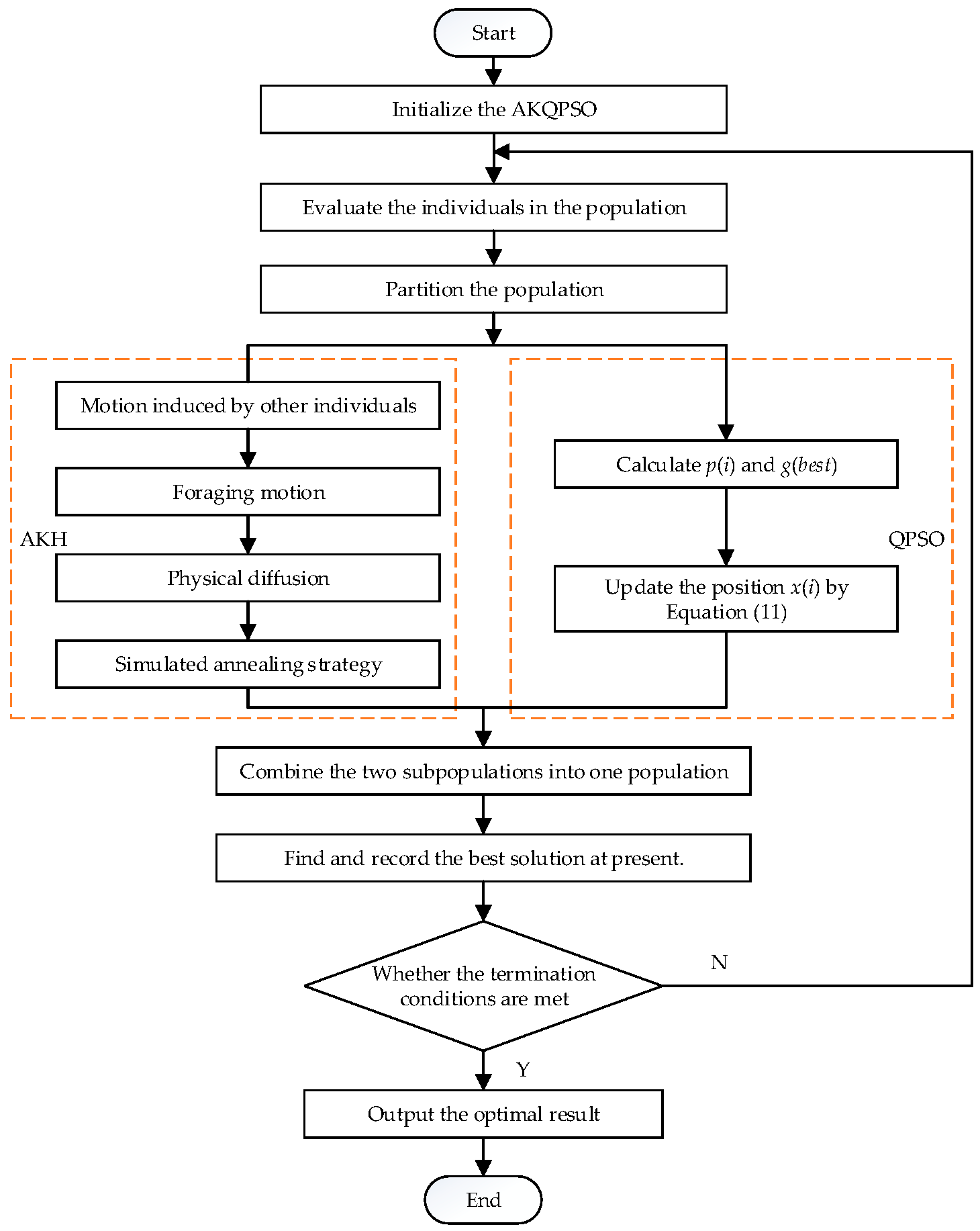
Figure 1. Framework of annealing krill quantum particle swarm optimization (AKQPSO).
Mathematics 08 01403 g001
Figure 2. Accuracy of AKQPSO and other algorithms on all problems.
Mathematics 08 01403 g002
Figure 3. Accuracy of AKQPSO and other algorithms on problem 1: Storn’s Chebyshev polynomial fitting problem. BBKH, biogeography-based krill herd; DEKH, differential evolution KH; QKH, quantum-behaved KH; SKH, stud KH; CCS, chaotic cuckoo search; VNBA, variable neighborhood bat algorithm; BBO, biogeography-based optimization; GA, genetic algorithm.
Mathematics 08 01403 g003
Figure 4. Accuracy of AKQPSO and other algorithms on problem 2: inverse Hilbert matrix problem.
Mathematics 08 01403 g004
Figure 5. Accuracy of AKQPSO and other algorithms on problem 3: Lennard–Jones minimum energy cluster.
Mathematics 08 01403 g005
Figure 6. Accuracy of AKQPSO and other algorithms on problem 4: Rastrigin’s function.
Mathematics 08 01403 g006
Figure 7. Accuracy of AKQPSO and other algorithms on problem 5: Griewangk’s function.
Mathematics 08 01403 g007
Figure 8. Accuracy of AKQPSO and other algorithms on problem 6: Weierstrass function.
Mathematics 08 01403 g008
Figure 9. Accuracy of AKQPSO and other algorithms on problem 7: modified Schwefel’s function.
Mathematics 08 01403 g009
Figure 10. Accuracy of AKQPSO and other algorithms on problem 8: expanded Schaffer’s F6 function.
Mathematics 08 01403 g010
Figure 11. Accuracy of AKQPSO and other algorithms on problem 9: happy cat function.
Mathematics 08 01403 g011
Figure 12. Accuracy of AKQPSO and other algorithms on problem 10: Ackley function.
Mathematics 08 01403 g012
Figure 13. Ratio of AKQPSO over other algorithms in the first group.
Mathematics 08 01403 g013
Figure 14. Ratio of AKQPSO over other algorithms in the second group.
Mathematics 08 01403 g014
Figure 15. Ratio of AKQPSO over other algorithms in the third group.
Mathematics 08 01403 g015
Figure 16. Ratio of AKQPSO over other algorithms in the fourth group.
Mathematics 08 01403 g016
Figure 17. The different subpopulations in different problems. (a) The different subpopulations in problems 1–10 and (b) the different subpopulations in problems 2–10.
Mathematics 08 01403 g017aMathematics 08 01403 g017b
Table 1. The basic parameters of the 100-Digit Challenge.
No.Functions F i * = F i ( x * ) DSearch Range
1Storn’s Chebyshev Polynomial Fitting Problem19(−8192–8192)
2Inverse Hilbert Matrix Problem116(−16,384–16,384)
3Lennard–Jones Minimum Energy Cluster118(−4–4)
4Rastrigin’s Function110(−100–100)
5Griewangk’s Function110(−100–100)
6Weierstrass Function110(−100–100)
7Modified Schwefel’s Function110(−100–100)
8Expanded Schaffer’s F6 Function110(−100–100)
9Happy Cat Function110(−100–100)
10Ackley Function110(−100–100)
Table 2. Parameter settings.
ParametersNmax_genmax_run
Value507500100
Table 3. The minimum value of annealing krill quantum particle swarm optimization (AKQPSO) and other algorithms in the 100-Digit Challenge. BBKH, biogeography-based krill herd; DEKH, differential evolution KH; QKH, quantum-behaved KH; SKH, stud KH; CCS, chaotic cuckoo search; VNBA, variable neighborhood bat algorithm; BBO, biogeography-based optimization; GA, genetic algorithm. (The table results retain ten decimal places.).
AlgorithmProblem 1Problem 2Problem 3
AKQPSO
(Algorithm 3)
10,893.3861385383215.68327663021.3068652046
BBKH291,803.2852933580613.71350868785.9027057769
DEKH975,339.7308122220708.06013381566.5872946609
QKH47,583.9014728552404.44166821852.1853645745
SKH1,773,168.4809322700402.72431665568.0692567398
CCS211,411.5538712060358.917537527212.4818284785
VNBA2,550,944.5550316900816.80713913504.6163144446
BBO72,287.9373622652311.81243778942.9209583205
GA8,009,879.02068729002209.19046602929.7547945042
AlgorithmProblem 4Problem 5Problem 6
AKQPSO
(Algorithm 3)
4.03983226951.04346963131.1185826442
BBKH17.79004438801.88523678643.9551854227
DEKH29.40885672321.95070219603.1953451545
QKH7.11334246312.06953623813.1213610789
SKH50.95488723561.935082591910.2543233489
CCS61.46045301353.45831117716.6010211976
VNBA24.72781993973.02512956915.7134938818
BBO17.42062591981.09719645902.5154932374
GA53.94443607652.71265732126.2420012291
AlgorithmProblem 7Problem 8Problem 9
AKQPSO
(Algorithm 3)
121.89323752702.31313240151.0715438957
BBKH779.40662296614.38465917271.3554069744
DEKH1060.03871289324.45099694711.3614909209
QKH195.07703636402.57113878681.2989726797
SKH1348.82134075474.87952871641.5980935412
CCS2247.44066025395.40026263501.6453371395
VNBA644.63344555354.14779327071.3950038682
BBO950.80186329393.59415246561.2098037868
GA1276.45653721454.23931601291.3580083289
AlgorithmProblem 10--
AKQPSO
(Algorithm 3)
21.0237707978--
BBKH21.6420368754--
DEKH21.6383024320--
QKH21.1582649016--
SKH21.6017549654--
CCS21.9603961872--
VNBA21.0799825759--
BBO21.9988888954--
GA21.4392031521--
Table 4. The different subpopulations in the AKQPSO algorithm.
λProblem 1Problem 2Problem 3Problem 4Problem 5
0.149,649.1118923043371.56257001591.40917995996.96975434261.1082189445
0.2133,608.1106469210370.04730399791.40913584393.98487717131.0983396055
0.310,893.3861385383215.68327663021.30686520464.03983226951.0434696313
0.453,539.2035950009346.10600257161.40913472884.97983622841.0588561989
0.586,346.3589566716424.47954429041.40914979735.97479528551.0564120753
0.682,979.4098834243422.24837235071.40947903595.04574810231.0861547616
0.799,948.7393233432609.38443845397.70578975807.96470836181.0885926731
0.8172,794.7224327620462.14828986521.409154613013.93446270441.0689273036
0.929,013.1541012323412.47768657573.94042202348.95972992621.0642761100
λProblem 6Problem 7Problem 8Problem 9Problem 10
0.11.4704093392401.18550670183.01180250921.095818763221.1048204811
0.21.2289194470336.43126754922.79878167241.096816766121.0708288643
0.31.1185826442121.89323752702.31313240151.071543895721.0237707978
0.42.6943320338119.53371698122.32990262641.101075837821.0389405345
0.52.9771884111209.55781143142.52179680331.125727525021.0587530353
0.62.5706601162253.12115509583.52276295321.135312727121.0976573470
0.71.4737157145187.58958218153.08849495251.134460565221.1144506567
0.81.5487741806144.35026336173.16125744481.155349725221.0835644844
0.94.0000000000131.27070353294.02090189511.161550399021.0768903380