New Analytical Model Used in Finite Element Analysis of Solids Mechanics


Abstract
1. Introduction
- choosing generalized coordinates (which do not need to be Cartesian coordinates);
- calculating kinetic energy;
- establishing generalized forces.
2. Preliminary
- is the velocity of the arbitrary chosen point;
- is the velocity of the origin of the mobile reference frame;
- is the rotation matrix (transform a vector from the mobile reference frame to the fixed reference frame);
- is the matrix of the shape functions depending on the type of finite element used;
- is the position vector of a current point in the local reference frame;
- is the vector of the generalized coordinates;
- is the vector of the generalized velocity;
- with the index L, a size is noted (vector, matrix), with the components expressed in the local reference frame, and with G, a size with the components expressed in the global reference frame.
3. Hamiltonian Equations for a Finite Element
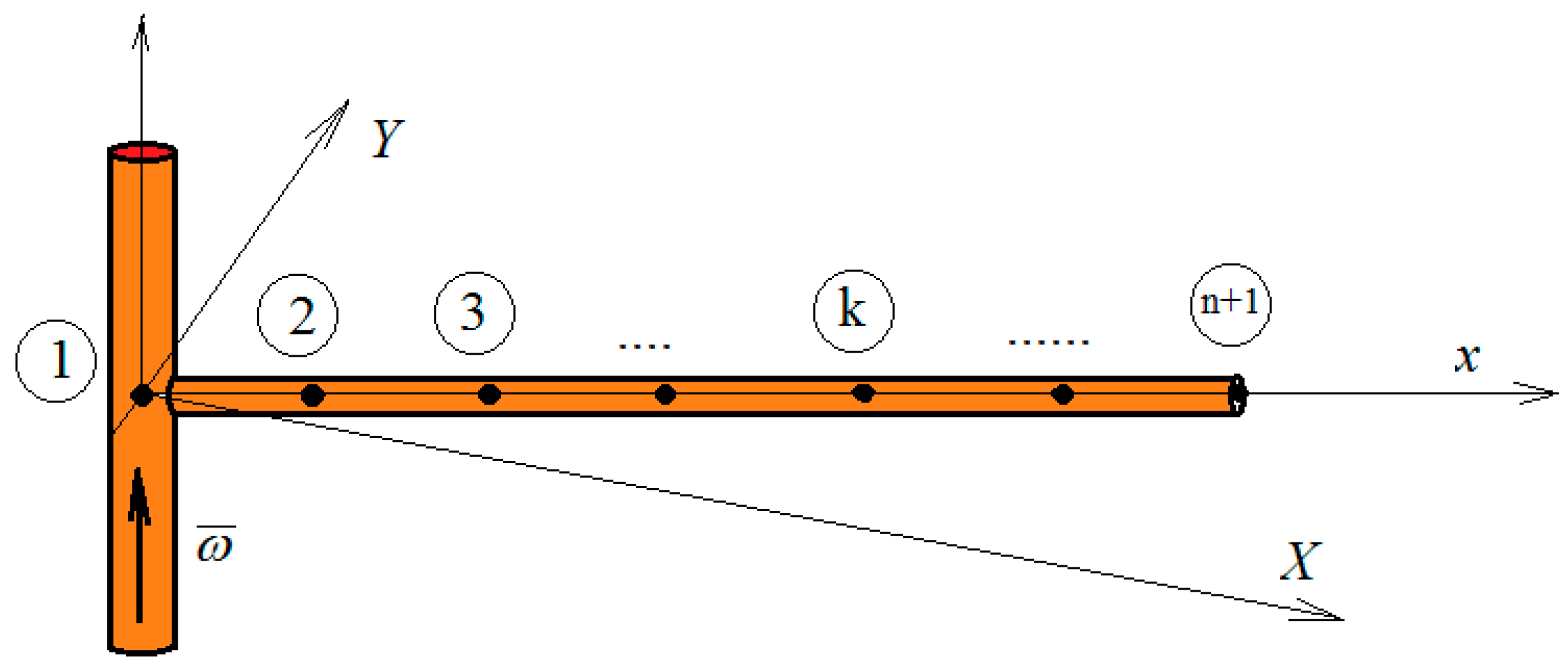
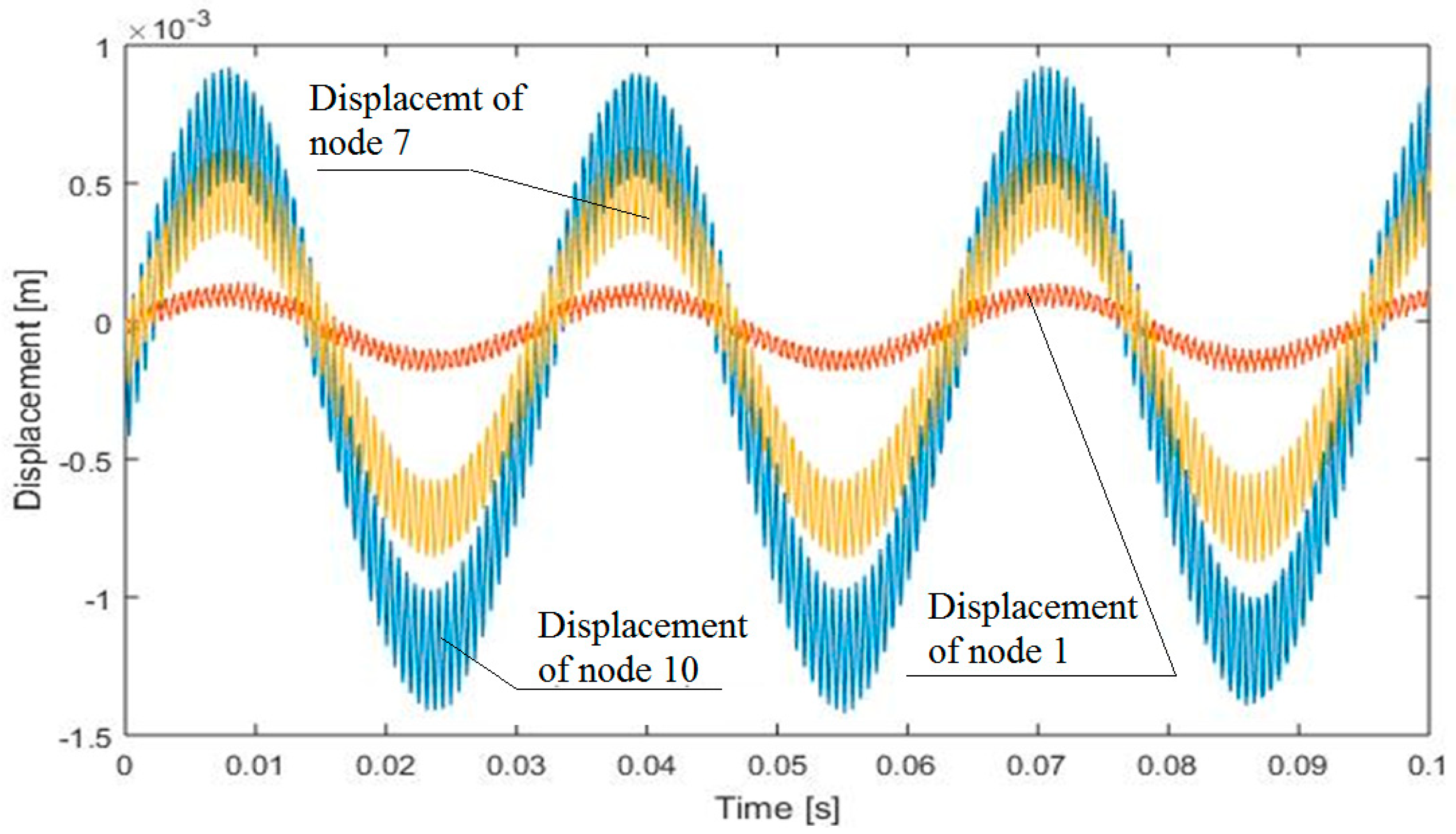
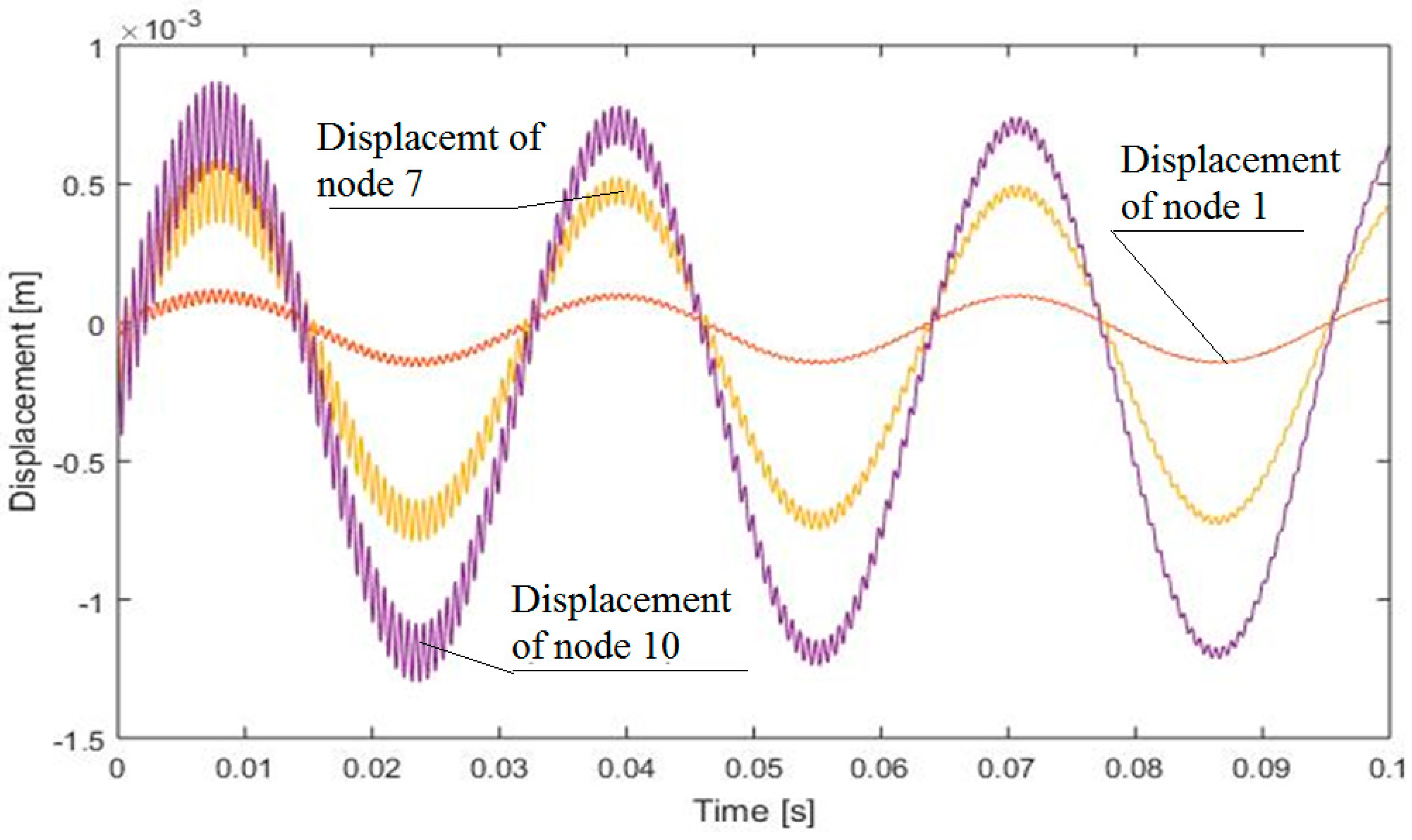
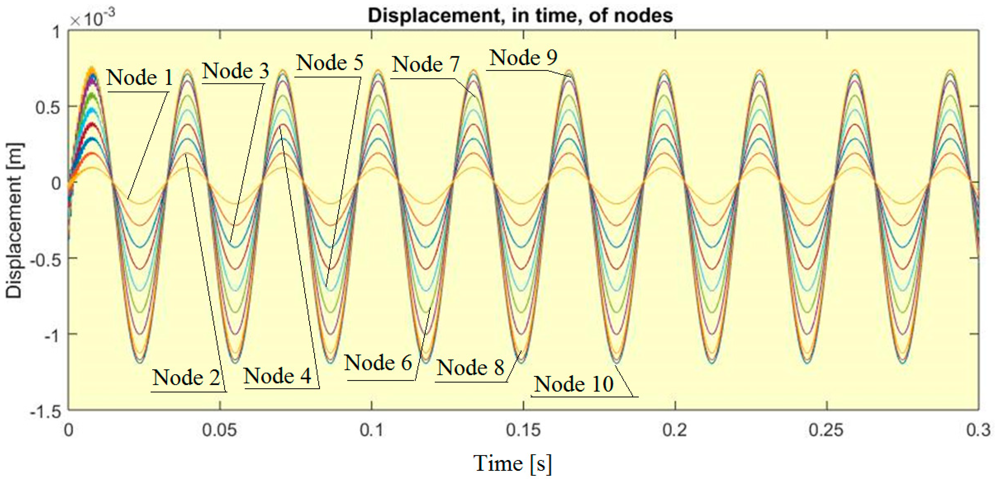
4. Examples
- a.
- Rotating beam
- b.
- Beam in a general planar motion
- c.
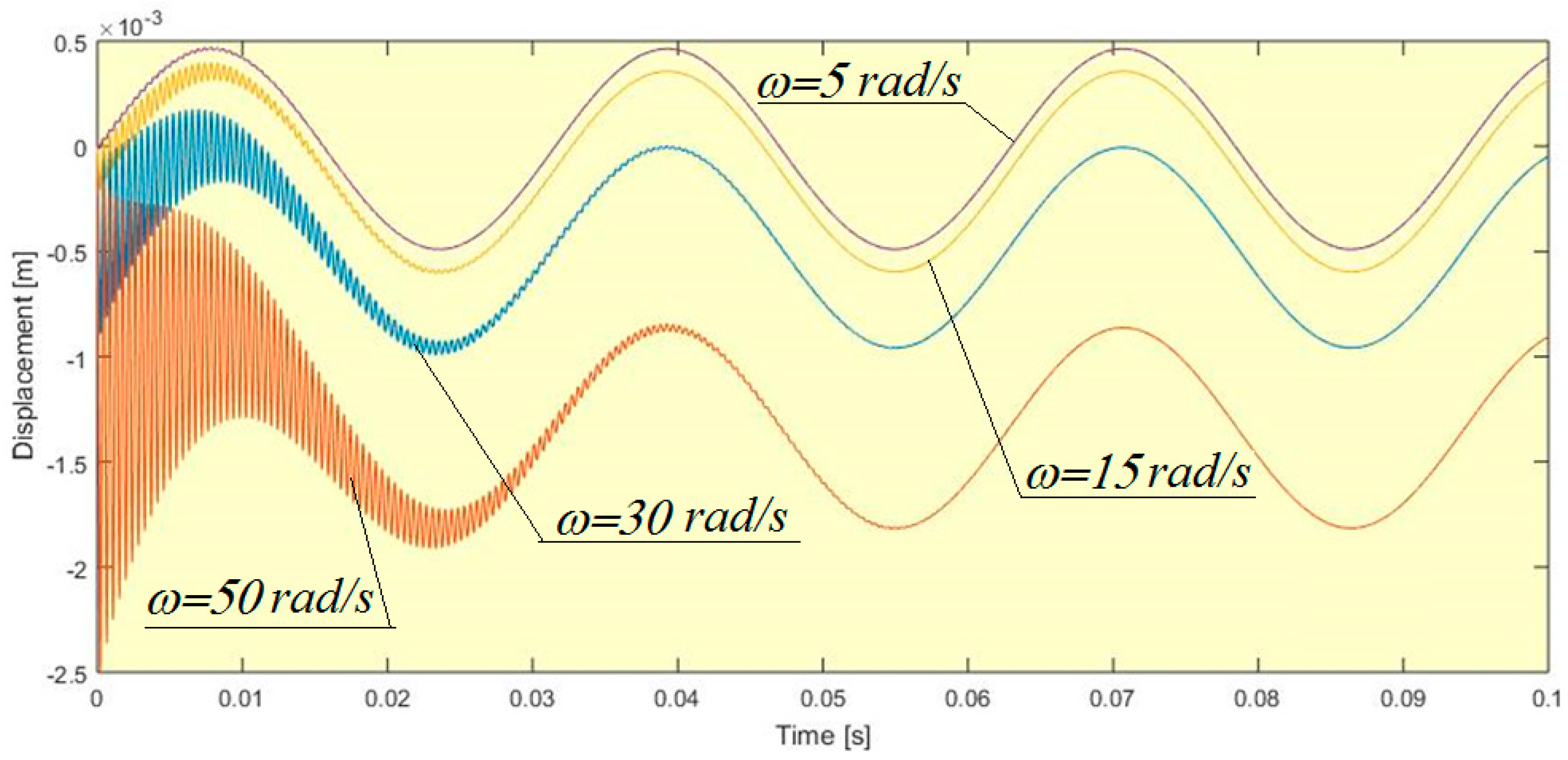
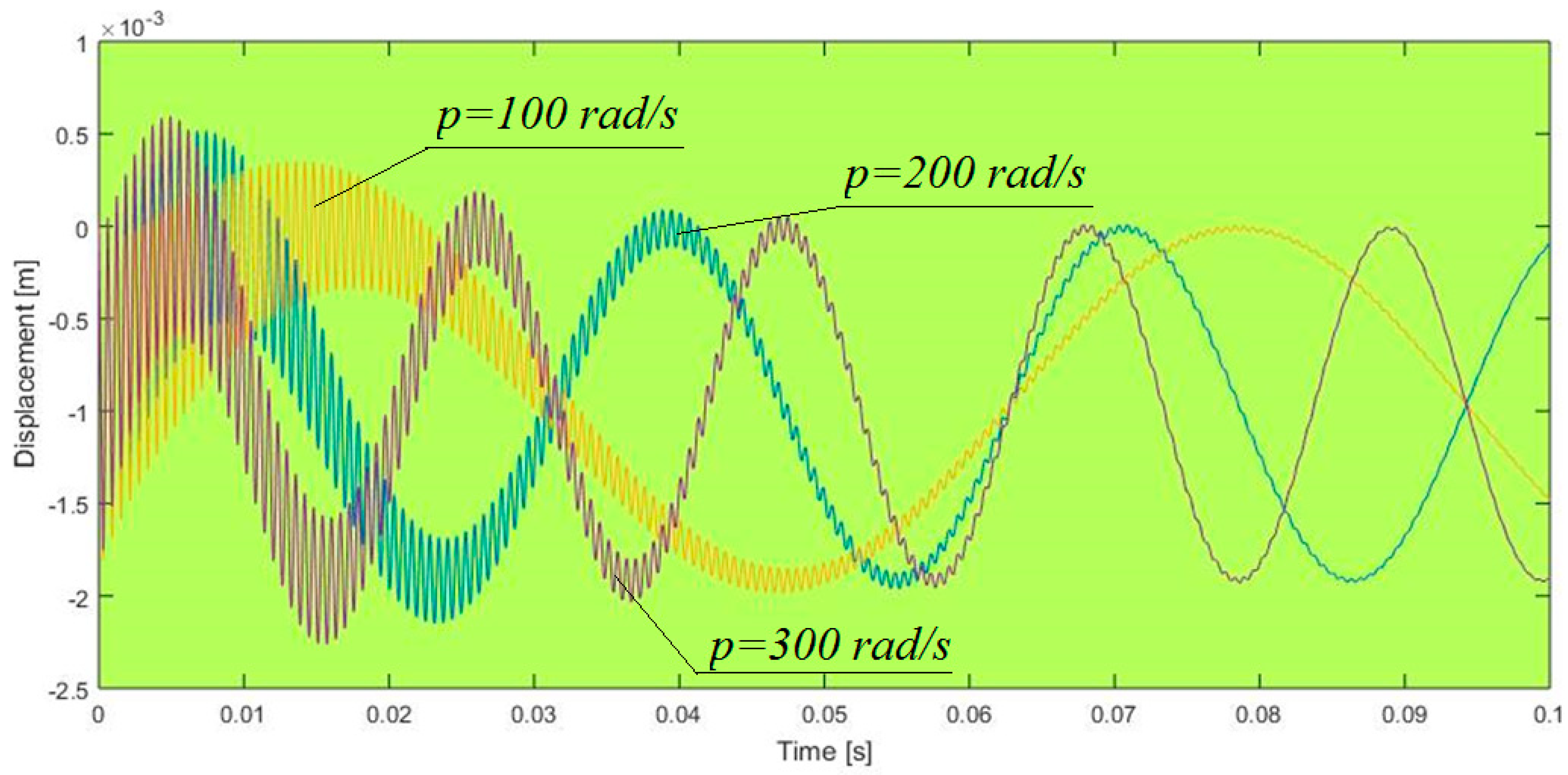
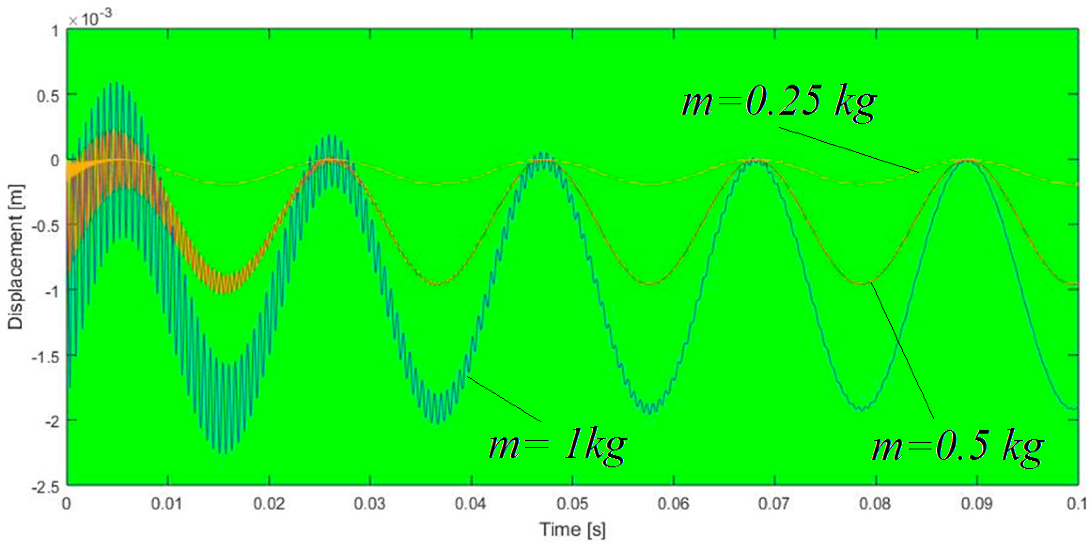
- Analysis of the influence of different parameters on the obtained solutions
5. Conclusions and Discussions
Author Contributions
Funding
Acknowledgments
Conflicts of Interest
Appendix A
Appendix A.1. Kinetic Energy
Appendix A.2. Potential Energy
Appendix A.3. Work
Appendix A.4. Lagrangian Equation
Appendix A.5. Generalized Momentum
Appendix A.6. Lagrange’s Equation
References
- Lagrange, J.L. Mecanique Analitique; Vve Desaint: Paris, France, 1788. [Google Scholar]
- Gibbs, J.W. On the fundamental formulae of dynamics. Am. J. Math. 1879, 2, 49–64. [Google Scholar] [CrossRef]
- Appell, P. Sur une forme générale des equations de la dynamique. J. Reine Angew. Math. 1900, 1900, 310–319. [Google Scholar]
- Hamilton, R.W. Second Essay on a General Method in Dynamics. In Phylosophical Transaction of the Royal Society, Part I; Wilkins, D.R., Ed.; Royal Society: London, UK, 1835; pp. 95–144. [Google Scholar]
- Maggi, G.A. Princippi della Teoria Matematica del Movimento dei Corpi: Corso di Meccanica Razionale; Ulrico Hoepli: Milano, Italy, 1896. [Google Scholar]
- Kane, T.T. Dynamic of Nonholonomic Systems, Transaction of ASME. J. Appl. Mech. 1961, 83, 574–578. [Google Scholar] [CrossRef]
- Haug, E.J. Extension of Maggi and Kane Equations to Holonomic Dynamic Systems. J. Comput. Nonlinear Dyn. 2018, 13, 121003. [Google Scholar] [CrossRef]
- Malvezzi, F.; Matarazzo Orsino, R.M.; Hess Coelho, T.A. Lagrange’s, Maggi’s and Kane’s equations to the dynamic modelling of serial manipulator. In DINAME 2017, Proceedings of the XVII International Symposium on Dynamic Problems of Mechanics, 5–10 March 2017; ABCM: São Sebastião, SP, Brazil, 2017. [Google Scholar]
- Wasfy, T.M.; Noor, A.K. Computational strategies for flexible multibody systems. ASME Appl. Mech. Rev. 2003, 56, 553–613. [Google Scholar] [CrossRef]
- Ursu-Fisher, N. Elements of Analytical Mechanics; House of Science Book Press: Cluj-Napoca, Romania, 2015. [Google Scholar]
- Negrean, I.; Kacso, K.; Schonstein, C.; Duca, A. Mechanics. Theory and Applications; UTPRESS: Cluj-Napoca, Romania, 2012. [Google Scholar]
- Mirtaheri, S.M.; Zohoor, H. The Explicit Gibbs-Appell Equations of Motion for Rigid-Body Constrained Mechanical System. In Proceedings of the 6th RSI International Conference on Robotics and Mechatronics (ICRoM), Tehran, Iran, 23–25 October 2018; pp. 304–309. [Google Scholar]
- Korayem, M.H.; Dehkordi, S.F. Motion equations of cooperative multi flexible mobile manipulator via recursive Gibbs-Appell formulation. Appl. Math. Model. 2019, 65, 443–463. [Google Scholar] [CrossRef]
- Vlase, S.; Negrean, I.; Marin, M.; Scutaru, M.L. Energy of Accelerations Used to Obtain the Motion Equations of a Three-Dimensional Finite Element. Symmetry 2020, 12, 321. [Google Scholar] [CrossRef]
- Amengonu, Y.H.; Kakad, Y.P. Dynamics and control for Constrained Multibody Systems modeled with Maggi’s equation: Application to Differential Mobile Robots Part II. In Proceedings of the 27th International Conference on CADCAM, Robotics and Factories of the Future, London, UK, 22–24 July 2014; Volume 65, p. 012018. [Google Scholar]
- Ladyzynska-Kozdras, E. Application of the Maggi equations to mathematical modeling of a robotic underwater vehicle as an object with superimposed non-holonomic constraints treated as control laws. Mechatron. Syst. Mech. Mater. 2012, 180, 152–159. [Google Scholar] [CrossRef]
- De Jalon, J.G.; Callejo, A.; Hidalgo, A.F. Efficient Solution of Maggi’s Equations. J. Comput. Nonlinear Dyn. 2012, 7, 021003. [Google Scholar] [CrossRef]
- Vlase, S.; Marin, M.; Scutaru, M.L. Maggi’s Equations Used in the Finite Element Analysis of the Multibody Systems with Elastic Elements. Mathematics 2020, 8, 399. [Google Scholar] [CrossRef]
- Wang, J.T.; Huston, R.L. Kane’s equations with undetermined multipiers-application to constrained multibody systems. ASME J. Appl. Mech. 1987, 54, 424–429. [Google Scholar] [CrossRef]
- Kane, T.R.; Levinson, D.A. Formulation of Equations of Motion for Complex Spacecraft. J. Guid. Control 1980, 3, 99–112. [Google Scholar] [CrossRef]
- Kane, T.R.; Levinson, D.A. Multibody Dynamics. J. Appl. Mech. 1983, 50, 1071–1078. [Google Scholar] [CrossRef]
- Vlase, S.; Negrean, I.; Marin, M.; Nastac, S. Kane’s Method-Based Simulation and Modeling Robots with Elastic Elements, Using Finite Element Method. Mathmatics 2020, 8, 805. [Google Scholar] [CrossRef]
- Dowell, E. Hamilton’s principle and Hamilton’s equations with holonomic and non-holonomic constraints. Nonlinear Dyn. 2017, 88, 1093–1097. [Google Scholar] [CrossRef]
- Tong, M.M. Flexible Multibody Dynamics Formulation by Hamilton’s Equations. In Proceedings of the ASME International Mechanical Engineering Congress and Exposition, Vancouver, BC, Canada, 12–18 November 2010; Volume 8, pp. 725–734. [Google Scholar]
- Qiao, Y.F.; Zhang, Y.L.; Han, G.C. Form invariance of Hamilton’s canonical equations of a nonholonomic mechanical system. Acta Phys. Sin. 2003, 52, 1051–1056. [Google Scholar]
- Erdman, A.G.; Sandor, G.N.; Oakberg, A. A General Method for Kineto-Elastodynamic Analysis and Synthesis of Mechanisms. J. Eng. Ind. 1972, 94, 1193–1205. [Google Scholar] [CrossRef]
- Bahgat, B.M.; Willmert, K.D. Finite Element Vibrational Analysis of Planar Mechanisms. Mech. Mach. Theory 1976, 11, 47–71. [Google Scholar] [CrossRef]
- Bagci, C. Elastodynamic Response of Mechanical Systems using Matrix Exponential Mode Uncoupling and Incremental Forcing Techniques with Finite Element Method. In Proceedings of the Sixth Word Congress on Theory of Machines and Mechanisms, New Delhi, India, 15–20 December1983; p. 472. [Google Scholar]
- Cleghorn, W.L.; Fenton, E.G.; Tabarrok, K.B. Finite Element Analysis of High-Speed Flexible Mechanisms. Mech. Mach. Theory 1981, 16, 407–424. [Google Scholar] [CrossRef]
- Vlase, S.; Marin, M.; Öchsner, A.; Scutaru, M.L. Motion equation for a flexible one-dimensional element used in the dynamical analysis of a multibody system. Contin. Mech. Thermodyn. 2019. [Google Scholar] [CrossRef]
- Vlase, S. Dynamical Response of a Multibody System with Flexible Elements with a General Three-Dimensional Motion. Rom. J. Phys. 2012, 57, 676–693. [Google Scholar]
- Deu, J.-F.; Galucio, A.C.; Ohayon, R. Dynamic responses of flexible-link mechanisms with passive/active damping treatment. Comput. Struct. 2008, 86, 258–265. [Google Scholar] [CrossRef]
- Hou, W.; Zhang, X. Dynamic analysis of flexible linkage mechanisms under uniform temperature change. J. Sound Vib. 2009, 319, 570–592. [Google Scholar] [CrossRef]
- Neto, M.A.; Ambrósio, J.A.C.; Leal, R.P. Composite materials in flexible multibody systems. Comput. Methods Appl. Mech. Eng. 2006, 195, 6860–6873. [Google Scholar] [CrossRef]
- Itu, C.; Oechsner, A.; Vlase, S.; Marin, M. Improved rigidity of composite circular plates through radial ribs. Proc. Inst. Mech. Eng. Part L—J. Mater. Des. Appl. 2019, 233, 1585–1593. [Google Scholar] [CrossRef]
- Marin, M.; Ellahi, R.; Chirilă, A. On solutions of Saint-Venant’s problem for elastic dipolar bodies with voids. Carpathian J. Math. 2017, 33, 219–232. [Google Scholar]
- Figueroa, H.; Carinena, J.F. Hamiltonian versus Lagrangian formulations of supermechanics. J. Phys. A Math. Gen. 1997, 30, 2705–2724. [Google Scholar]
- Naudet, J.; Lefeber, D.; Daerden, F.; Terze, Z. Forward Dynamics of Open-Loop Multibody Mechanisms Using an Efficient Recursive Algorithm Based on Canonical Momenta. Multibody Syst. Dyn. 2003, 10, 45–59. [Google Scholar] [CrossRef]
- Kim, J.; Kim, D. A quadratic temporal finite element method for linear elastic structural dynamics. Math. Comput. Simul. 2015, 117, 68–88. [Google Scholar] [CrossRef]
- Xue, Y.; Weng, D.W.; Chen, L.Q. Methods of analytical mechanics for exact Cosserat elastic rod dynamics. Acta Phys. Sin. 2013, 62, 044601. [Google Scholar] [CrossRef]
- MATLAB. Available online: https://de.mathworks.com/help/matlab/ (accessed on 29 July 2020).
- Dubowsky, S.; Gardner, T.N. Dynamic interactions of link elasticity and clearance connections in planar mechanical systems. ASME J. Eng. Ind. 1975, 97, 652–661. [Google Scholar] [CrossRef]
- Midha, A.; Erdman, A.G.; Forhib, D.A. Finite element approach to mathematical modeling of high-speed elastic linkages. Mech. Mach. Theory 1978, 13, 603–618. [Google Scholar] [CrossRef]
- Midha, A.; Erdman, A.G.; Forhib, D.A. A computationally efficient numerical algorithm for the transient response of high-speed elastic linkages. ASME J. Mech. Des. 1979, 101, 138–148. [Google Scholar] [CrossRef]
- Blejwas, T.E. The simulation of elastic mechanisms using kinematic constraints and Lagrange multipliers. Mech. Mach. Theory 1981, 16, 441–445. [Google Scholar] [CrossRef]
- Bricout, J.N.; Debus, J.C.; Micheau, P. A finite element model for the dynamics of flexible manipulators. Mech. Mach. Theory 1990, 25, 119–128. [Google Scholar] [CrossRef]
- Meirovitch, L.; Kwak, M.K. Dynamics and control of spacecraft with retargeting flexible antennas. J. Guid. Control Dyn. 1990, 13, 241–248. [Google Scholar] [CrossRef]
- Fattah, A.; Angeles, J.; Misra, A.K. Dynamics of a 3-DOF spatial parallel manipulator with flexible links. In Proceedings of the 1995 IEEE International Conference on Robotics and Automation, Nagoya, Japan, 21–27 May 1995; pp. 627–632. [Google Scholar]
- Pereira, M.S.; Ambrosio, J.A.C.; Dias, J.P. Crashworthiness analysis and design using rigid-flexible multibody dynamics with application to train vehicles. Int. J. Numer. Methods Eng. 1997, 40, 655–687. [Google Scholar] [CrossRef]
- Turcic, D.A.; Midha, A. Generalized equations of motion for the dynamic analysis of elastic mechanism systems. ASME J. Dyn. Syst. Meas. Control 1984, 106, 243–248. [Google Scholar] [CrossRef]
- Turcic, D.A.; Midha, A. Dynamic analysis of elastic mechanism systems, Part I: Applications. ASME J. Dyn. Syst. Meas. Control 1984, 106, 249–254. [Google Scholar] [CrossRef]
- Bakr, E.M.; Shabana, A.A. Geometrically nonlinear analysis of multibody systems. Comput. Struct. 1986, 23, 739–751. [Google Scholar] [CrossRef]
- Changizi, K.; Shabana, A.A. A recursive formulation for the dynamics analysis of open loop deformable multibody systems. J. Appl. Acoust. 1988, 55, 687–693. [Google Scholar] [CrossRef]
- Modi, V.J.; Suleman, A.; Ng, A.C.; Morita, Y. An approach to dynamics and control of orbiting flexible structures. Int. J. Numer. Methods Eng. 1991, 32, 1727–1748. [Google Scholar] [CrossRef]
- Pereira, M.S.; Proenca, P.L. Dynamic analysis of spatial flex ible multibody systems using joint coordinates. Int. J. Numer. Methods Eng. 1991, 32, 1799–1821. [Google Scholar] [CrossRef]
- Pradhan, S.; Modi, V.J.; Misra, A.K. Order N formulation for flexible multibody systems in tree topology: Lagrangian approach. J. Guid. Control Dyn. 1997, 20, 665–672. [Google Scholar] [CrossRef]
- Metaxas, D.; Koh, E. Flexible multibody dynamics and adaptive finite element techniques for model synthesis and estimation. Comput. Methods Appl. Mech. Eng. 1996, 136, 1–25. [Google Scholar] [CrossRef]
- Huang, S.J.; Wang, T.Y. Structural dynamics analysis of spatial robots with finite element method. Comput. Struct. 1993, 46, 703–716. [Google Scholar] [CrossRef]
- Smaili, A.A. A three-node finite beam element for dynamic analysis of planar manipulators with flexible joints. Mech. Mach. Theory 1993, 28, 193–206. [Google Scholar] [CrossRef]
- Meek, J.L.; Liu, H. Nonlinear dynamics analysis of flexible beams under large overall motions and the flexible manipulator simulation. Comput. Struct. 1995, 56, 1–14. [Google Scholar] [CrossRef]
- Pan, Y.C.; Scott, R.A.; Ulsoy, G.A. Dynamic modeling and simulation of flexible robots with prismatic joints. ASME J. Mech. Des. 1990, 112, 307–314. [Google Scholar] [CrossRef]
- Cavin, R.K.; Dusto, A.R. Hamilton’s principle: Finite element methods and flexible body dynamics. AIAA J. 1977, 15, 1684–1690. [Google Scholar] [CrossRef]
- Chang, L.W.; Hamilton, J.F. Kinematics of robotic manipulators with flexible links using and equivalent rigid link system ERLS model. ASME J. Dyn. Syst. Meas. Control 1991, 113, 48–54. [Google Scholar] [CrossRef]
- Serna, M.A. A simple and efficient computational approach for the forward dynamics of elastic robots. J. Rob. Syst. 1989, 6, 363–382. [Google Scholar] [CrossRef]
- Fung, R.F. Dynamic analysis of the flexible connecting rod of slider-crank mechanism with time-dependent boundary effect. Comput. Struct. 1997, 63, 79–90. [Google Scholar] [CrossRef]
- Huang, Y.; Lee, C.S.G. Generalization of Newton-Euler formulations of dynamic equations to nonrigid manipulators. ASME J. Dyn. Syst. Meas. Control 1988, 110, 308–315. [Google Scholar] [CrossRef]
- Iura, M.; Atluri, S.N. Dynamic analysis of planar flexible beams with finite rotations by using inertial and rotating frames. Comput. Struct. 1955, 55, 453–462. [Google Scholar] [CrossRef]
- Bauchau, O.A.; Damilano, G.; Theron, N.J. Numerical integration of non-linear elastic multibody systems. Int. J. Numer. Methods Eng. 1955, 38, 2727–2751. [Google Scholar] [CrossRef]
- Bauchau, O.A.; Choi, J.-Y.; Bottasso, C.L. On the modeling of shells in multibody dynamics. Multibody Syst. Dyn. 2002, 8, 459–489. [Google Scholar] [CrossRef]


| Term of Hamiltonian Equation | |
|---|---|
| 0 | |
| 0 | |
| 0 | |
| 0 | |
| 0 | |
| 0 | |
| Node 1 | Node 2 | ||||||
|---|---|---|---|---|---|---|---|
| 306.4 | 894.2 | 1923 | 8991 | 252.4 | 670.2 | 1480 | 7325 |
| 263.3 | 1006 | 1763 | 9962 | 242.3 | 845.8 | 899.5 | 9851 |
| 253.8 | 1194 | 2448 | 14,580 | 325.9 | 1015 | 2233 | 14,490 |
| 346.4 | 1243 | 2445 | 13,980 | 259.2 | 996.5 | 2421 | 12,610 |
| 315.5 | 1538 | 2957 | 16,330 | 355.2 | 1296 | 3000 | 14,260 |
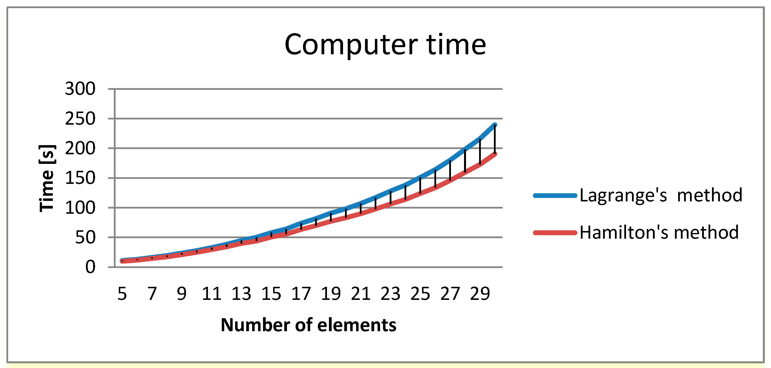
| Number of elements | 5 | 10 | 15 | 20 | 25 |
| Lagrange’s method. Time (s) | 31 | 84 | 176 | 291 | 460 |
| Hamilton’s method. Time (s) | 28 | 68 | 139 | 224 | 322 |
© 2020 by the authors. Licensee MDPI, Basel, Switzerland. This article is an open access article distributed under the terms and conditions of the Creative Commons Attribution (CC BY) license (http://creativecommons.org/licenses/by/4.0/).
Share and Cite
Vlase, S.; Nicolescu, A.E.; Marin, M. New Analytical Model Used in Finite Element Analysis of Solids Mechanics. Mathematics 2020, 8, 1401. https://doi.org/10.3390/math8091401
Vlase S, Nicolescu AE, Marin M. New Analytical Model Used in Finite Element Analysis of Solids Mechanics. Mathematics. 2020; 8(9):1401. https://doi.org/10.3390/math8091401
Chicago/Turabian StyleVlase, Sorin, Adrian Eracle Nicolescu, and Marin Marin. 2020. "New Analytical Model Used in Finite Element Analysis of Solids Mechanics" Mathematics 8, no. 9: 1401. https://doi.org/10.3390/math8091401
APA StyleVlase, S., Nicolescu, A. E., & Marin, M. (2020). New Analytical Model Used in Finite Element Analysis of Solids Mechanics. Mathematics, 8(9), 1401. https://doi.org/10.3390/math8091401