An Improvement on the Upper Bounds of the Partial Derivatives of NURBS Surfaces

Abstract

The Non-Uniform Rational B-spline (NURBS) surface not only has the characteristics of the rational Bézier surface, but also has changeable knot vectors and weights, which can express the quadric surface accurately. In this paper, we investigated new bounds of the first- and second-order partial derivatives of NURBS surfaces. A pilot study was performed using inequality theorems and degree reduction of B-spline basis functions. Theoretical analysis provides simple forms of the new bounds. Numerical examples are performed to illustrate that our method has sharper bounds than the existing ones.

1. Introduction

The bounds on derivatives of NURBS surfaces have very important applications for Computer Aided Geometric Design (CAGD). For example, various algorithms for parametric curves and surfaces, such as linear approximation, subdivision of trimmed surfaces and segmentation errors of surfaces [1], depend on knowing the bounds of the estimated derivatives. Therefore, a tight upper bound on the derivative contributes to improve the efficiency and stability of these algorithms.

For this reason, many researchers have concentrated on the bounds of the derivatives of representative curves and surfaces. Since Floater [2] gave a classical inequality to estimate the upper bounds of the first-order derivatives of Bézier curves, several improved results have been derived for rational Bézier curves and surfaces [3,4,5,6,7,8,9,10,11,12,13,14,15,16,17,18]. Huang [19] obtained the bounds on derivatives of rational Bézier curves. Cao [20], Hu [21] and Liu [22] presented methods for the bounds estimation of the second-order derivatives of rational triangular Bézier surfaces. Wang [23] obtained the upper bounds expression of the third-order derivatives of the rational Bézier curves by moving control points. To the best of our knowledge, few published articles have studied the bounds of derivatives on NURBS surfaces. This usually involves tedious expressions and knot vector analysis of B-spline basis functions. Unfortunately, it is difficult to generalize the study of derivative bounds on NURBS surfaces to the second-order derivative form due to the complex product representation. One available reference for obtaining the bounds of the derivatives of rational Bézier surfaces was presented by Selimovic [24]. Subsequently, Wang [25] estimated the partial derivative bounds for NURBS surfaces.

As the case stands, the NURBS surfaces with the characteristics of changeable knot vectors and weights are a natural extension of the Bézier surfaces. They control the curves of the object surfaces better than traditional mesh modeling. Furthermore, NURBS surfaces are considered to be more suitable for complex surface modeling and surface subdivision. Obtaining a tight upper bound of the second-order derivative can achieve a more perfect surface tessellation without increasing the amount of data.

In this paper, we deduce powerful unified bounds of the first- and second-order derivatives of NURBS surfaces based on the degree reduction of the B-spline basis functions, geometrical properties of NURBS surfaces and some basic inequality skills. The bounds on first-order derivatives of NURBS surfaces given in this paper are sharper than the existing ones [24,25]. Furthermore, they are less affected by the change of weights, knot vectors and control points. We also present a novel estimation method for the bounds of the second-order derivatives of NURBS surfaces. The new proposed approach is more practical in application. For instance, the new method can also be applied to rational Bézier surfaces, which means it can be used for estimating derivatives of surfaces without judging the surface type. Moreover, tighter upper bounds than some existed methods are also given in our method. In the piecewise linear approximation algorithm proposed by Filip et al. [26], a more convergent derivative bound can make the result of surface subdivision more accurate. Both theoretical analysis and numerical examples are provided to verify the superiority of the proposed method.

The rest of the paper is organized as follows. Section 2 briefly reviews the definition and properties of NURBS surfaces. Furthermore, it introduces the preliminary lemma that will be needed later. Section 3 deduces new bounds on the first- and second-order partial derivatives of NURBS surfaces. The numerical experiments are shown in Section 4 to compare the existing bounds and the new bounds. Finally, Section 5 concludes this paper.

2. Preliminary

Before deducing the main results, we briefly introduce some definitions and notations in this section.

The degree reduction method of B-spline functions is given below. Let $T=\left(t_0,t_1,\cdots ,t_n\right)$ be a knot vector. B-spline function of order $p$ (degree $k$) is defined as

$$\{\begin{array}{l}{N}_{i,1}\left(t\right)=\{\begin{array}{l}1\mathrm{for}t\in \left[t_i,t_{i+1}\right)\\ 0\mathrm{otherwise}\end{array}\\ N_{i,p}\left(t\right)=\frac{t-t_i}{t_{i+p-1}-t_i}{N}_{i,p-1}\left(t\right)+\frac{t_{i+p}-t}{t_{i+p}-t_{i+1}}{N}_{i+1,p-1}\left(t\right)\\ wherep=k+1,0\le i\le n-p,2\le p\le n,\frac{0}{0}=0\end{array}$$

(1)

Let $P_0,P_1,\cdots ,P_m\left(P_i\in R^d\right)$ be $m+1$ control points, $T=\left(t_0,t_1,\cdots ,t_{m+p+1}\right)$ knot vector. B-spline curve of order $p$ for control points $P_i$ and knot vector $T$ is defined as

$$C\left(t\right)={\displaystyle \sum _{i=0}^m{P}_i{N}_{i,p}\left(t\right)}$$

(2)

The first derivative of the B-spline curve defined in (2) can be evaluated as

$$\{\begin{array}{l}C{\left(t\right)}^{\prime }={\displaystyle \sum _{i=0}^m{N}_{i,p}{\left(t\right)}^{\prime }{P}_i}\\ N_{i,p}{\left(t\right)}^{\prime }=\frac{p-1}{t_{i+p-1}-t_i}{N}_{i,p-1}\left(t\right)-\frac{p-1}{t_{i+p}-t_{i+1}}{N}_{i+1,p-1}\left(t\right)\end{array}$$

(3)

In cases where the first and the last p knots are identical, we have

$$\{\begin{array}{l}{N}_{0,p-1}\left(t\right)\equiv 0,t_{p-1}-t_0=0\\ N_{m+1,p-1}\left(t\right)\equiv 0,t_{m+p}-t_{m+1}=0\end{array}$$

Equation (3) is proved in [27]. Using (1), (2) and (3), the degree of B-spline functions is reduced. The degree reduction method of B-spline curves can be extended to B-spline surfaces. Both $u$ parameter direction and $v$ parameter direction need to use a method of degree reduction. Projecting the result of the B-spline surfaces onto the $\omega =1$ hyperplane, the result of the NURBS surface is obtained.

The NURBS book [28] provides the definition of a NURBS surface. Given the control points $P_{ij}$ and positive weights ${\omega }_{ij}$, a NURBS surface $R(u,v)$ of order $p\times q$ is defined by

$$R(u,v)=\frac{{\displaystyle \sum _{i=0}^n{\displaystyle \sum _{j=0}^m{N}_{i,p}(u)N_{j,q}(v)P_{ij}{\omega }_{ij}}}}{{\displaystyle \sum _{i=0}^n{\displaystyle \sum _{j=0}^m{N}_{i,p}(u)N_{j,q}(v){\omega }_{ij}}}}=\frac{P(u,v)}{W(u,v)}$$

(4)

where the B-spline basis functions $N_{i,p}(u)$, $N_{j,q}(v)$ ($i=0,\cdots ,n$, $j=0,\cdots ,m$) are defined on the knot vectors $[u_0,u_1,\cdots ,u_{n+p}]$ and $[v_0,v_1,\cdots ,v_{m+q}]$, respectively, and assume that the two knot vectors satisfy the endpoint conditions:

$$u_0=u_1\cdots =u_{p-1},u_{n+1}=u_{n+2}\cdots =u_{n+p},v_0=v_1\cdots =v_{q-1},v_{m+1}=v_{m+2}\cdots =v_{m+q}$$

(5)

According to the properties of B-spline basis functions, some basic derivative formulas of NURBS surfaces are listed in Appendix A; $P_u$, $P_v$, $P_{uu}$, $P_{vv}$, $P_{uv}$, $W_u$, $W_v$, $W_{uu}$, $W_{vv}$, and $W_{uv}$ are included. It should also be noted that the notations $Q_{ij}^u$, $Q_{ij}^v$, $R_{ij}^u$, $R_{ij}^v$, $Q_{ij}^{uv}$, $d_{ij}^u$, $d_{ij}^v$, $e_{ij}^u$, $e_{ij}^v$, $d_{ij}^{uv}$, ${\overline{\omega }}_{ij}^u$, ${\overline{\omega }}_{ij}^v$, ${\tilde{\omega }}_{ij}^u$, ${\tilde{\omega }}_{ij}^v$, ${\overline{d}}_{ij}^u$ and ${\overline{d}}_{ij}^v$ are introduced in Appendix A to simplify the expressions, and these notations will appear repeatedly in later theorems and proofs. In addition, in the remainder of this paper, if the scope of an intermediate variable is not given, the variables $i$, $I$, and $s$ are always from 0 to $n$, and the variable $j$, $J$, and $t$ are from 0 to $m$.

Additionally, to estimate the derivative bounds of NURBS surfaces, the following lemma will be used for the proof of our results. A similar lemma was used in references [7,19] to estimate upper bounds for Bézier curves.

Lemma 1.

If $a_i(t)\ge 0$, $b_i(t)>0$, $c_i(t)\ge 0$, $i=0,\cdots ,n$, parameter $t\in \left[t_1,t_2\right]$, and $\forall t\in \left[t_1,t_2\right]$, ${\displaystyle \sum _{i=0}^n{c}_i(t)b_i(t)}>0$, then $\frac{{\displaystyle \sum _{i=0}^n{c}_i(t)a_i(t)}}{{\displaystyle \sum _{i=0}^n{c}_i(t)b_i(t)}}\le \underset{i,t\in [t_1,t_2]}{\max }\frac{a_i(t)}{b_i(t)}$.

3. Estimation of Bounds on the Partial Derivatives of NURBS Surfaces

In this section, we provide the bounds on the first- and second-order partial derivatives of the NURBS surfaces.

3.1. Bounds on the First-Order Partial Derivatives

Theorem 1.

For a NURBS surface $R(u,v)$ of order $p\times q$ defined by (4), a bound on the magnitude of the first-order partial derivative with respect to $u$ can be expressed as

$$\Vert R_u\Vert \le (p-1)\underset{1\le i\le n,j,I,J}{\max }\frac{\Vert \left(P_{ij}-P_{IJ}\right){\omega }_{ij}-\left(P_{i-1j}-P_{IJ}\right){\omega }_{i-1j}\Vert }{\left(u_{i+p-1}-u_i\right)\min \left\{{\omega }_{ij},{\omega }_{i-1j}\right\}}$$

(6)

Proof. 

The first-order partial derivative of a NURBS surface with respect to $u$ can be written as

$$R_u=\frac{P_{u}W-P{W}_u}{W^2}$$

(7)

Rewrite the numerator and denominator of $\frac{P_{u}W-P{W}_u}{W^2}$, so that we can get the bound by applying Lemma 1. By replacing $P_u$ and $W_u$ in (7) with (A1) and (A6), it follows that

$$P_{u}W-P{W}_u=\left(p-1\right){\displaystyle \sum _{i=1}^n{\displaystyle \sum _{j=0}^m{\displaystyle \sum _{I=0}^n{\displaystyle \sum _{J=0}^m{N}_{i,p-1}(u)N_{j,q}(v)N_{I,p}(u)N_{J,q}(v)\left(Q_{ij}^u-P_{IJ}{d}_{ij}^u\right){\omega }_{IJ}}}}}$$

(8)

Rearranging all the terms in $W^2$ by applying (A11), rewrite $W^2$ as

$$W^2={\displaystyle \sum _{i=1}^n{\displaystyle \sum _{j=0}^m{\displaystyle \sum _{I=0}^n{\displaystyle \sum _{J=0}^m{N}_{i,p-1}(u)N_{j,q}(v)N_{I,p}(u)N_{J,q}(v){\overline{\omega }}_{ij}^u{\omega }_{IJ}}}}}$$

(9)

Now, considering the bound of $\Vert R_u\Vert$, we have

$$\begin{array}{l}\Vert R_u\Vert =\Vert \frac{P_{u}W-P{W}_u}{W^2}\Vert =\frac{\left(p-1\right)\Vert {\displaystyle \sum _{i=1}^n{\displaystyle \sum _{j=0}^m{\displaystyle \sum _{I=0}^n{\displaystyle \sum _{J=0}^m{N}_{i,p-1}(u)N_{j,q}(v)N_{I,p}(u)N_{J,q}(v)\left(Q_{ij}^u-P_{IJ}{d}_{ij}^u\right){\omega }_{IJ}}}}}\Vert }{{\displaystyle \sum _{i=1}^n{\displaystyle \sum _{j=0}^m{\displaystyle \sum _{I=0}^n{\displaystyle \sum _{J=0}^m{N}_{i,p-1}(u)N_{j,q}(v)N_{I,p}(u)N_{J,q}(v){\overline{\omega }}_{ij}^u{\omega }_{IJ}}}}}}\\ \le \left(p-1\right)\underset{1\le i\le n,j,I,J}{\max }\frac{\Vert Q_{ij}^u-P_{IJ}{d}_{ij}^u\Vert }{{\overline{\omega }}_{ij}^u}\\ \le \left(p-1\right)\underset{1\le i\le n,j,I,J}{\max }\frac{\Vert \left(P_{ij}-P_{IJ}\right){\omega }_{ij}-\left(P_{i-1j}-P_{IJ}\right){\omega }_{i-1j}\Vert }{\left(u_{i+p-1}-u_i\right)\min \left\{{\omega }_{ij},{\omega }_{i-1j}\right\}}\end{array}$$

(10)

Similarly,

$$\Vert R_v\Vert \le (q-1)\underset{i,1\le j\le m,I,J}{\max }\frac{\Vert \left(P_{ij}-P_{IJ}\right){\omega }_{ij}-\left(P_{ij-1}-P_{IJ}\right){\omega }_{ij-1}\Vert }{\left(v_{j+q-1}-v_j\right)\min \left\{{\omega }_{ij},{\omega }_{ij-1}\right\}}$$

(11)

□

3.2. Bounds on the Second-Order Partial Derivatives

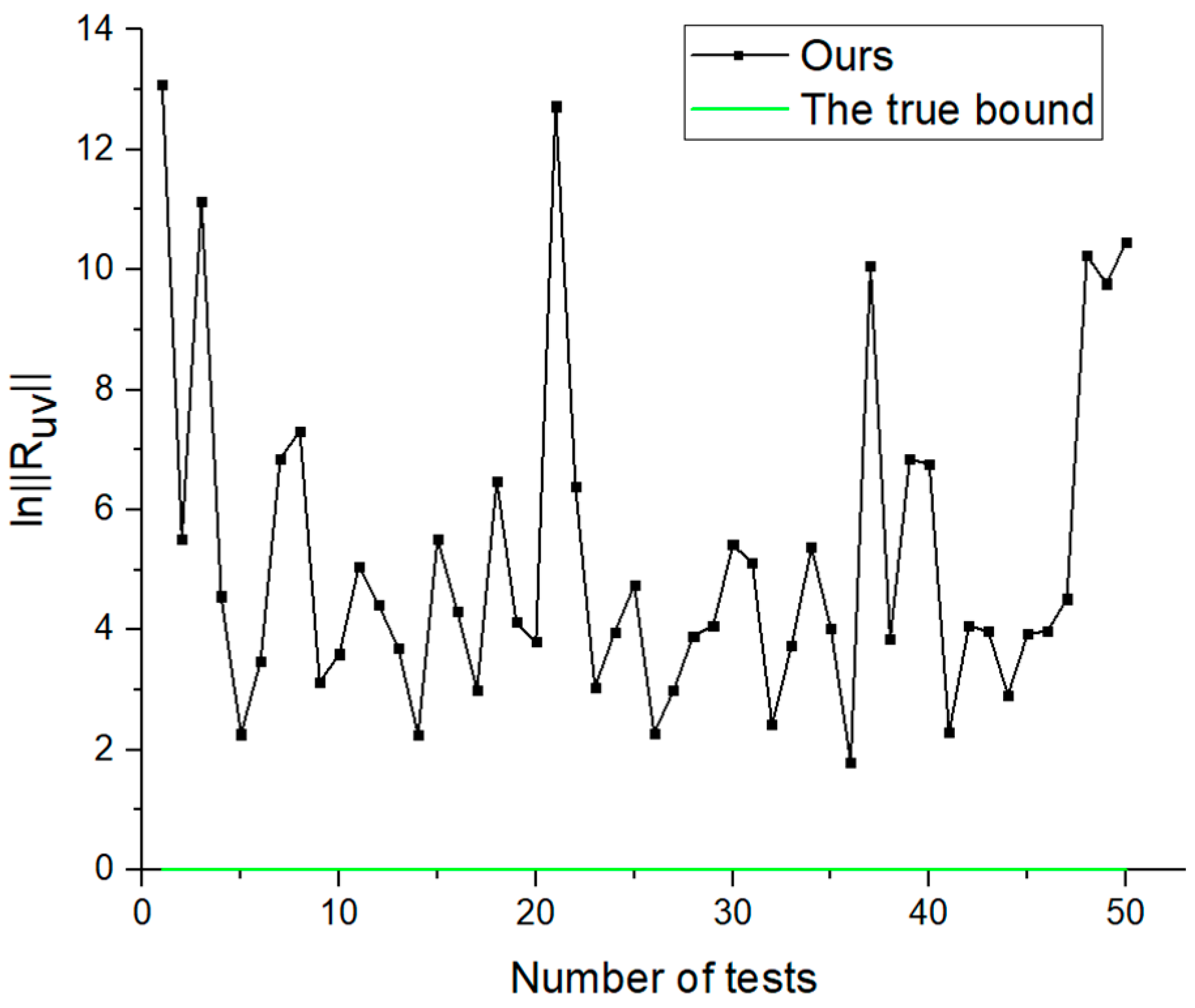
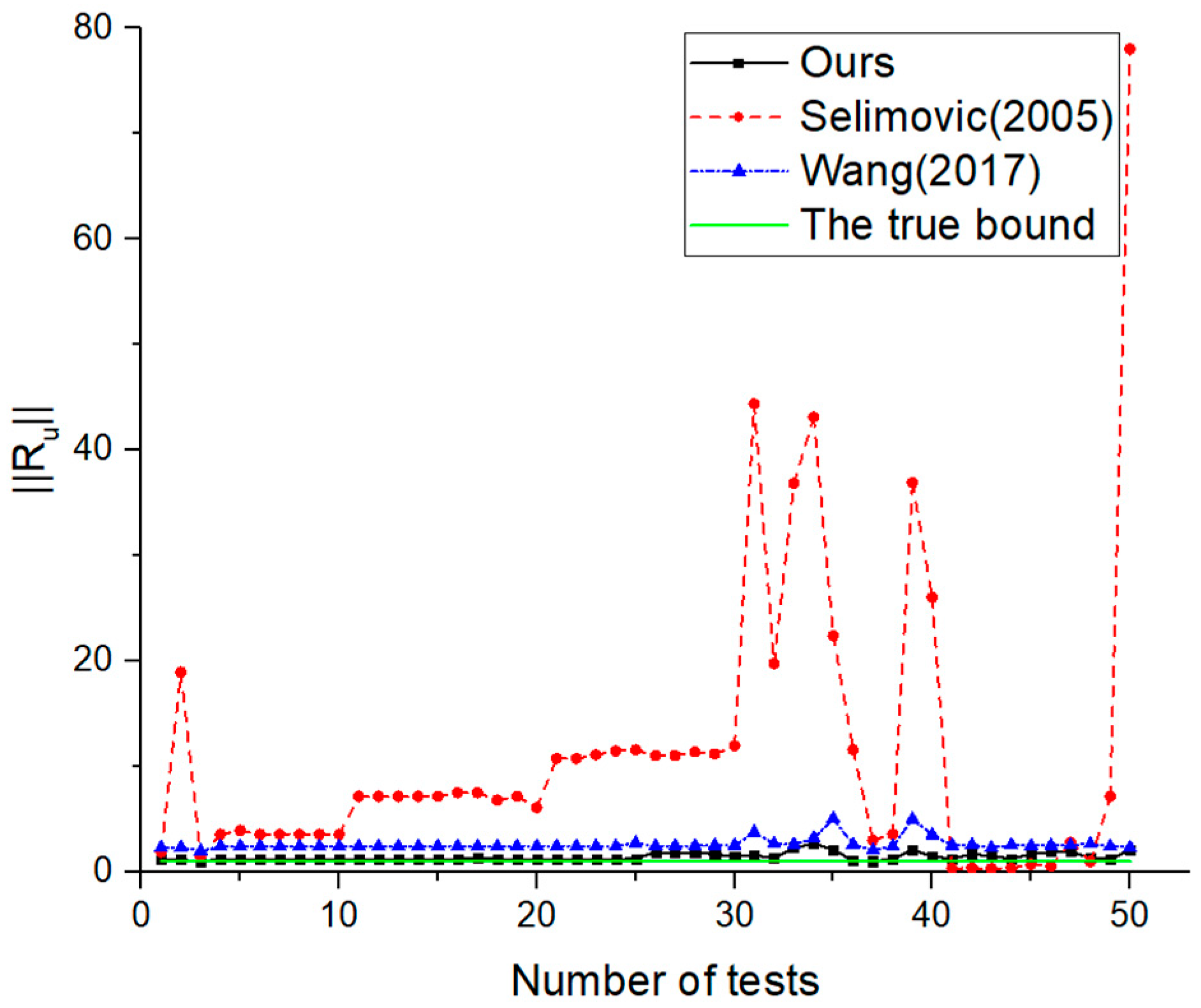
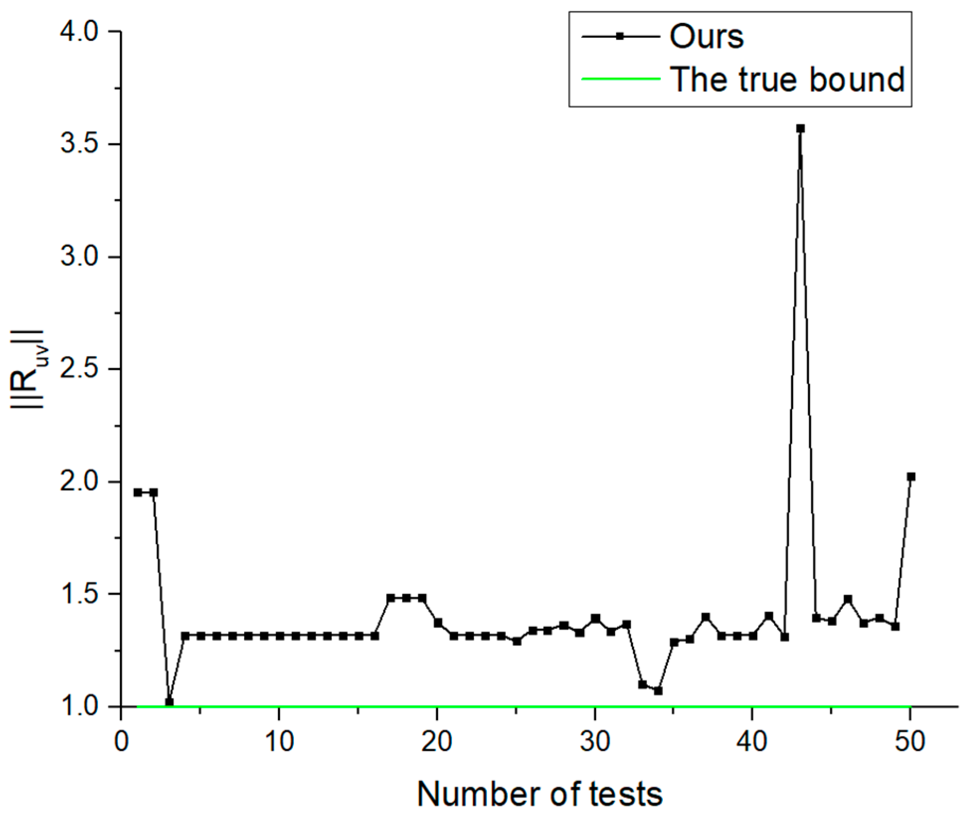
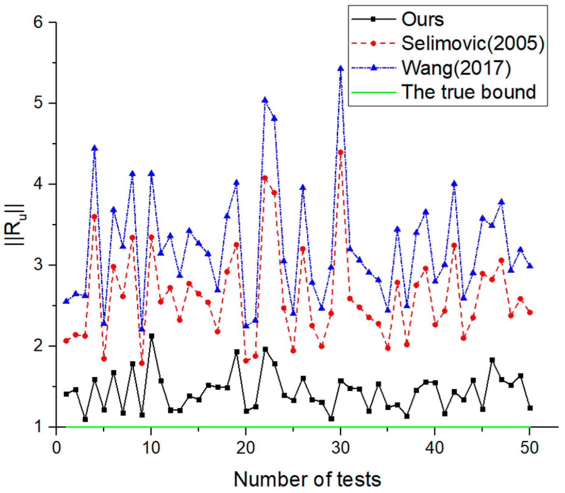
Theorem 2.

For a NURBS surface $R(u,v)$ of order $p\times q$ defined by (4), a bound on the magnitude of the second-order partial derivative with respect to $u$ can be expressed as

$$\Vert R_{uu}\Vert <(p-1)\underset{i,j,1\le I\le n,J,2\le s\le n,t}{\max }\frac{\max \Vert F_{ijIJst}^{uu}(u)\Vert }{\min \{{\omega }_{IJ},{\omega }_{I-1J}\}·\min \{{\omega }_{st},{\omega }_{s-1t},{\omega }_{s-2t}\}}$$

(12)

where each component of $F_{ijIJst}^{uu}(u)$ denotes a linear polynomial of $u$,

$$F_{ijIJst}^{uu}(u)=(p-2)\left(R_{st}^u-P_{ij}{e}_{st}^u\right){\overline{\omega }}_{IJ}^u-2(p-1)\left(Q_{IJ}^u-P_{ij}{d}_{IJ}^u\right){\overline{d}}_{st}^u$$

(13)

Proof. 

The second-order partial derivative of a NURBS surface with respect to $u$ can be written as

$$R_{uu}=\frac{\left(P_{uu}W-P{W}_{uu}\right)W-2\left(P_{u}W-P{W}_u\right)W_u}{W^3}$$

(14)

First, we need to estimate the bound of $\Vert R_{uu}\Vert$ using Lemma 1. The following theorem will use the main results (A1), (A3), (A6), (A8), (A11), (A13), and (A15) in Appendix A. Following degree reduction of B-spline functions and rearrange subscripts, we have

$$W^3={\displaystyle \sum _{i=0}^n{\displaystyle \sum _{j=0}^m{\displaystyle \sum _{I=1}^n{\displaystyle \sum _{J=0}^m{\displaystyle \sum _{s=2}^n{\displaystyle \sum _{t=0}^m{N}_{i,p}(u)N_{j,q}(v)N_{I,p-1}(u)N_{J,q}(v)N_{s,p-2}(u)N_{t,q}(v){\omega }_{ij}{\overline{\omega }}_{IJ}^u{\tilde{\omega }}_{st}^u}}}}}}$$

(15)

$$\begin{array}{l}\left(P_{uu}W-P{W}_{uu}\right)W=\\ \left(p-1\right)\left(p-2\right){\displaystyle \sum _{i=0}^n{\displaystyle \sum _{j=0}^m{\displaystyle \sum _{I=1}^n{\displaystyle \sum _{J=0}^m{\displaystyle \sum _{s=2}^n{\displaystyle \sum _{t=0}^m{N}_{i,p}(u)N_{j,q}(v)N_{I,p-1}(u)N_{J,q}(v)N_{s,p-2}(u)N_{t,q}(v){\omega }_{ij}{\overline{\omega }}_{IJ}^u\left(R_{st}^u-P_{ij}{e}_{st}^u\right)}}}}}}\end{array}$$

(16)

$$\begin{array}{l}\left(P_{u}W-P{W}_u\right)W_u=\\ {\left(p-1\right)}^2{\displaystyle \sum _{i=0}^n{\displaystyle \sum _{j=0}^m{\displaystyle \sum _{I=1}^n{\displaystyle \sum _{J=0}^m{\displaystyle \sum _{s=2}^n{\displaystyle \sum _{t=0}^m{N}_{i,p}(u)N_{j,q}(v)N_{I,p-1}(u)N_{J,q}(v)N_{s,p-2}(u)N_{t,q}(v){\omega }_{ij}\left(Q_{IJ}^u-P_{ij}{d}_{IJ}^u\right){\overline{d}}_{st}^u}}}}}}\end{array}$$

(17)

$$\begin{array}{l}\left(P_{uu}W-P{W}_{uu}\right)W-2\left(P_{u}W-P{W}_u\right)W_u=\\ (p-1){\displaystyle \sum _{i=0}^n{\displaystyle \sum _{j=0}^m{\displaystyle \sum _{I=1}^n{\displaystyle \sum _{J=0}^m{\displaystyle \sum _{s=2}^n{\displaystyle \sum _{t=0}^m{N}_{i,p}}}}}}}(u)N_{j,q}(v)N_{I,p-1}(u)N_{J,q}(v)N_{s,p-2}(u)N_{t,q}(v)F_{ijIJst}^{uu}(u){\omega }_{ij}\end{array}$$

(18)

Before we estimate the bound of $\Vert R_{uu}\Vert$, the minimum value of ${\overline{\omega }}_{IJ}^u{\tilde{\omega }}_{st}^u$ should be given. It is easy to confirm that

$$\min {\overline{\omega }}_{IJ}^u=\min \frac{\left(u-u_I\right){\omega }_{IJ}+\left(u_{I+p-1}-u\right){\omega }_{I-1J}}{u_{I+p-1}-u_I}=\min \left\{{\omega }_{IJ},{\omega }_{I-1J}\right\}$$

(19)

$$\min {\tilde{\omega }}_{st}^u=\min \frac{\left(u-u_s\right){\overline{\omega }}_{st}^u+\left(u_{s+p-2}-u\right){\overline{\omega }}_{s-1t}^u}{u_{s+p-2}-u_s}\ge \min \left\{{\omega }_{st},{\omega }_{s-1t},{\omega }_{s-2t}\right\}$$

(20)

Hence

$${\overline{\omega }}_{IJ}^u{\tilde{\omega }}_{st}^u\ge \min \left\{{\omega }_{IJ},{\omega }_{I-1J}\right\}·\min \left\{{\omega }_{st},{\omega }_{s-1t},{\omega }_{s-2t}\right\}$$

(21)

Each component of $F_{ijIJst}^{uu}(u)$ is a linear polynomial of u. By estimating the maximum value of $\Vert F_{ijIJst}^{uu}(u)\Vert$, we obtain

$$\max \Vert F_{ijIJst}^{uu}(u)\Vert =\max \left\{\Vert F_{ijIJst}^{uu}(u_{\alpha })\Vert ,\Vert F_{ijIJst}^{uu}(u_{\beta })\Vert \right\}$$

(22)

where $[u_{\alpha },u_{\beta }]=[u_i,u_{i+p}]\cap [u_I,u_{I+p-1}]\cap [u_s,u_{s+p-2}]$; here, $[u_i,u_{i+p}]$, $[u_I,u_{I+p-1}]$ and $[u_s,u_{s+p-2}]$ are support intervals of B-spline basis functions $N_{i,p}(u)$, $N_{I,p-1}(u)$ and $N_{s,p-2}(u)$, and $0\le i\le n$, $1\le I\le n$, $2\le s\le n$. $[u_{\alpha },u_{\beta }]$ may be empty, but it does not affect the following results. It is easy to obtain $u_{\alpha }=\max \left\{u_i,u_I,u_s\right\}$ and $u_{\beta }=\min \left\{u_{i+p},u_{I+p-1},u_{s+p-2}\right\}$. □

Based on the above discussion, the bound of the partial derivative can be estimated by

$$\begin{array}{l}\Vert R_{uu}\Vert =\Vert \frac{\left(P_{uu}W-P{W}_{uu}\right)W-2\left(P_{u}W-P{W}_u\right)W_u}{W^3}\Vert \\ =\frac{\Vert (p-1){\displaystyle \sum _{i=0}^n{\displaystyle \sum _{j=0}^m{\displaystyle \sum _{I=1}^n{\displaystyle \sum _{J=0}^m{\displaystyle \sum _{s=2}^n{\displaystyle \sum _{t=0}^m{N}_{i,p}(t)N_{j,q}(t)N_{I,p-1}(t)N_{J,q}(t)N_{s,p-2}(t)N_{t,q}(t)F_{ijIJst}^{uu}(u){\omega }_{ij}}}}}}}\Vert }{{\displaystyle \sum _{i=0}^n{\displaystyle \sum _{j=0}^m{\displaystyle \sum _{I=1}^n{\displaystyle \sum _{J=0}^m{\displaystyle \sum _{s=2}^n{\displaystyle \sum _{t=0}^m{N}_{i,p}(t)N_{j,q}(t)N_{I,p-1}(t)N_{J,q}(t)N_{s,p-2}(t)N_{t,q}(t){\omega }_{ij}{\overline{\omega }}_{IJ}^u{\tilde{\omega }}_{st}^u}}}}}}}\\ \le (p-1)\underset{i,j,1\le I\le n,J,2⩽s\le n,t}{\max }\frac{\max \Vert F_{ijIJst}^{uu}(u)\Vert }{\min \left\{{\omega }_{IJ},{\omega }_{I-1J}\right\}·\min \left\{{\omega }_{st},{\omega }_{s-1t},{\omega }_{s-2t}\right\}}\end{array}$$

(23)

Due to the symmetric property of parameter u and v of NURBS surface, the bound on $R_{vv}$ can be derived in the same way as $R_{uu}$. It can be expressed as

$$\Vert R_{vv}\Vert \le \left(q-1\right)\underset{i,j,I,1\le J\le m,s,2\le t\le m}{\max }\frac{\max \Vert F_{ijIJst}^{vv}(v)\Vert }{\min \left\{{\omega }_{IJ},{\omega }_{IJ-1}\right\}·\min \left\{{\omega }_{st},{\omega }_{st-1},{\omega }_{st-2}\right\}}$$

(24)

where each component of $F_{ijIJst}^{vv}(v)$ is a linear polynomial of v,

$$F_{ijIJst}^{vv}(v)=(q-2)\left(R_{st}^v-P_{ij}{e}_{st}^v\right){\overline{\omega }}_{IJ}^v-2(q-1)\left(Q_{IJ}^v-P_{ij}{d}_{IJ}^v\right){\overline{d}}_{st}^v$$

(25)

From (22), it is easy to determine that

$$\max \Vert F_{ijIJst}^{vv}(v)\Vert =\max \left\{\Vert F_{ijIJst}^{vv}(v_{\alpha })\Vert ,\Vert F_{ijIJst}^{vv}(v_{\beta })\Vert \right\}$$

(26)

where $[v_{\alpha },v_{\beta }]=[v_j,v_{j+q}]\cap [v_J,v_{J+q-1}]\cap [v_t,v_{t+q-2}]$; here, $[v_j,v_{j+q}]$, $[v_J,v_{J+q-1}]$ and $[v_t,v_{t+q-2}]$ are support intervals of B-spline basis functions $N_{j,q}(v)$, $N_{J,q-1}(v)$ and $N_{t,q-2}(v)$, and $v_{\alpha }=\max \left\{v_j,v_J,v_t\right\}$, $v_{\beta }=\min \left\{v_{j+q},v_{J+q-1},v_{t+q-2}\right\}$.

In the following, we will derive the bound on the mixed partial derivative in a similar way.

Theorem 3.

For a NURBS surface $R(u,v)$ of order $p\times q$ defined by (4), its mixed partial derivative satisfies

$$\Vert R_{uv}\Vert \le (p-1)(q-1)\underset{i,j,1\le I\le n,J,s,1\le t\le m}{\max }\frac{\Vert F_{ijIJst}^{uv}\Vert }{\min \left\{{\omega }_{IJ},{\omega }_{I-1J}\right\}·\min \left\{{\omega }_{st},{\omega }_{st-1}\right\}}$$

(27)

where $F_{ijIJst}^{uv}$ is a constant vector and can be expressed by the control points, weights and knot vectors of the NURBS surface $R(u,v)$ explicitly as

$$F_{ijIJst}^{uv}=Q_{It}^{uv}{\omega }_{sJ}-Q_{IJ}^u{d}_{st}^v-Q_{st}^v{d}_{IJ}^u-P_{sJ}{\omega }_{sJ}{d}_{It}^{uv}+2P_{ij}{d}_{IJ}^u{d}_{st}^v$$

(28)

Proof. 

The mixed partial derivative of a NURBS surface can be expressed as

$$R_{uv}=\frac{P_{uv}{W}^2-P_u{W}_{v}W-P_v{W}_{u}W-P{W}_{uv}W+2P{W}_u{W}_v}{W^3}$$

(29)

We deal with the numerator and denominator of $R(u,v)$ separately. Applying (A11) and (A12), we have

$$W^3={\displaystyle \sum _{i=0}^n{\displaystyle \sum _{j=0}^m{\displaystyle \sum _{I=1}^n{\displaystyle \sum _{J=0}^m{\displaystyle \sum _{s=0}^n{\displaystyle \sum _{t=1}^m{N}_{i,p}(u)N_{j,q}(v)N_{I,p-1}(u)N_{J,q}(v)N_{s,p}(u)N_{t,q-1}(v){\omega }_{ij}{\overline{\omega }}_{IJ}^u{\overline{\omega }}_{st}^v}}}}}}$$

(30)

By recalling the definitions of ${\overline{\omega }}_{ij}^u$ and ${\overline{\omega }}_{ij}^v$ in (A11) and (A12), the minimum of ${\overline{\omega }}_{IJ}^u{\overline{\omega }}_{st}^v$ can be computed. We know that ${\overline{\omega }}_{ij}^u$ and ${\overline{\omega }}_{ij}^v$ are linear polynomials of u and v, respectively; thus, it is easy to obtain that

$${\overline{\omega }}_{IJ}^u\ge \min \left\{{\omega }_{IJ},{\omega }_{I-1J}\right\}$$

(31)

$${\overline{\omega }}_{st}^v\ge \min \left\{{\omega }_{st},{\omega }_{st-1}\right\}$$

(32)

Next, we substitute the expressions of (A1), (A2), (A5), (A6), (A7) and (A10) into the numerator of (29). Therefore, we find that

$$\begin{array}{l}{P}_{uv}{W}^2-P_u{W}_{v}W-P_v{W}_{u}W-P{W}_{uv}W+2P{W}_u{W}_v\\ =\left(p-1\right)\left(q-1\right){\displaystyle \sum _{i=0}^n{\displaystyle \sum _{j=0}^m{\displaystyle \sum _{I=1}^n{\displaystyle \sum _{J=0}^m{\displaystyle \sum _{s=0}^n{\displaystyle \sum _{t=1}^m{N}_{i,p}(u)N_{j,q}(v)N_{I,p-1}(u)}}}}}}{N}_{J,q}(v)N_{s,p}(u)N_{t,q-1}(v)\\ \left(Q_{It}^{uv}{\omega }_{sJ}-Q_{IJ}^u{d}_{st}^v-Q_{st}^v{d}_{IJ}^u-P_{sJ}{\omega }_{sJ}{d}_{It}^{uv}+2P_{ij}{d}_{IJ}^u{d}_{st}^v\right){\omega }_{ij}\\ =\left(p-1\right)\left(q-1\right){\displaystyle \sum _{i=0}^n{\displaystyle \sum _{j=0}^m{\displaystyle \sum _{I=1}^n{\displaystyle \sum _{J=0}^m{\displaystyle \sum _{s=0}^n{\displaystyle \sum _{t=1}^m{N}_{i,p}(u)N_{j,q}(v)N_{I,p-1}(u)}}}}}}{N}_{J,q}(v)N_{s,p}(u)N_{t,q-1}(v)F_{ijIJst}^{uv}{\omega }_{ij}\end{array}$$

(33)

Combing with (30), (31), (32) and (33), the following result is obtained.

$$\begin{array}{l}\Vert R_{uv}\Vert =\Vert \frac{P_{uv}{W}^2-P_u{W}_{v}W-P_v{W}_{u}W-P{W}_{uv}W+2P{W}_u{W}_v}{W^3}\Vert \\ \le (p-1)(q-1)\frac{{\displaystyle \sum _{i=0}^n{\displaystyle \sum _{j=0}^m{\displaystyle \sum _{I=1}^n{\displaystyle \sum _{J=0}^m{\displaystyle \sum _{s=0}^n{\displaystyle \sum _{t=1}^m{N}_{i,p}}}}}}}(u)N_{j,q}(v)N_{I,p-1}(u)N_{J,q}(v)N_{s,p}(u)N_{t,q-1}(v)\Vert F_{ijIJst}^{uv}\Vert {\omega }_{ij}}{{\displaystyle \sum _{i=0}^n{\displaystyle \sum _{j=0}^m{\displaystyle \sum _{I=1}^n{\displaystyle \sum _{J=0}^m{\displaystyle \sum _{s=0}^n{\displaystyle \sum _{t=1}^m{N}_{i,p}}}}}}}(u)N_{j,q}(v)N_{I,p-1}(u)N_{J,q}(v)N_{s,p}(u)N_{t,q-1}(v){\omega }_{ij}{\overline{\omega }}_{IJ}^u{\overline{\omega }}_{st}^v}\\ \le (p-1)(q-1)\underset{i,j,1\le I\le n,J,s,1\le t\le m}{\max }\frac{\Vert F_{ijIJst}^{uv}\Vert }{\min \{{\omega }_{IJ},{\omega }_{I-1J}\}·\min \{{\omega }_{st},{\omega }_{st-1}\}}\end{array}$$

(34)

□

4. Numeric Examples

In this section, numerical experiments are provided to show the correctness and superiority of the proposed bounds of the derivative of NURBS surfaces. In the following experiments, the ratios of the approximate bounds of the NURBS surface to their exact bounds instead of the true value are used for comparison. Let the parameter domain of a NURBS surface be $\left[a_1,a_2\right]\times \left[b_1,b_2\right]$. The repeated control points can be supplemented to ensure that the surface always meets the endpoint condition (5), and the properties of the surface will not change. The ground truth bound of a derivative is approximated by iteratively selecting the maximum value of the derivatives at the sampled points $\left\{\left(u,v\right)|u=a_1+i/100·(a_2-a_1),v=b_1+j/100·(b_2-b_1),0\le i,j\le 100\right\}$ on the surface. The horizontal axis represents the number of experiments, and the vertical axis means the ratio of the estimated bound to the exact bound. For each experiment, the closer the result is to the true bound (represented by the green line in the figure), the more accurate it is. All numeric examples are included in the Supplementary Materials.

Since our bounds of NURBS surfaces involve knot vectors, weights and control points, we compare ours with the results in Selimovic [24] and Wang [25] in three ways. In Figure 1 and Figure 2, we set the NURBS surface with control points $R=\left[\left(1,1,1\right),\left(1,1,2\right),\left(0,5,5\right),\left(4,3,2\right),\left(7,2,1\right),\left(6,2,1\right),\left(3,1,1\right),\left(8,6,3\right),\left(0,1,2\right)\right]$ and corresponding knot vectors $U=\left\{0,1,1.3,2.1,3.6,4.0\right\},V=\left\{0,0.8,1.2,2.3,3.1,4.2\right\}$. Weights are randomly generated in the interval [1,100]. This experiment was conducted 50 times. It can be seen that our results are closer to the true bounds than those in Selimovic [24] and Wang [25]. Moreover, the new bounds are less affected by fluctuations of weights. The effectiveness of the bounds on the second-order partial derivatives can also be seen in Figure 2.

The second comparison group (Figure 3 and Figure 4) has the same control points as the first group. The monotonic non-decreasing knot vectors of the NURBS surfaces are randomly sampled in interval $\left[0,300\right]$. Then the weights are defined as $\omega =\left[0.85,0.76,0.82,0.88,0.79,0.85,0.75,0.84,0.78\right]$. Again, this experiment was performed 50 times. It can be observed that our bounds are closer to the green line than the results in Selimovic [24] and Wang [25]. It is easy to conclude that the knot vector has little effect on our bounds, proving that our bounds are stronger than those in Selimovic [24] and Wang [25]. It is worth noting that the method in Selimovic [24] fails in some examples. The situation of the $\left|R_{uv}\right|$ also illustrates the superiority of the new bounds.

In the third comparison group (Figure 5 and Figure 6), we set knot vectors $U=\left\{0,1,1.3,2.1,3.6,4.0\right\}$, $V=\left\{0,0.8,1.2,2.3,3.1,4.2\right\}$ and weights $\omega =\left[0.85,0.76,0.82,0.88,0.79,0.85,0.75,0.84,0.78\right]$. Control points are randomly selected in the interval $\left[0,10\right]$. Similarly, the experiment was conducted 50 times. It can be concluded from the comparison that our bounds are sharper than the known bounds in Selimovic [24] and Wang [25], confirming that the new bounds are more stable.

A set of all randomly selected variables comparison group is also provided in Figure 7 and Figure 8. We first select the same examples as in Wang [25]. Then we extend these examples by changing the parameters. Weights are randomly generated in the interval $\left[1,100\right]$, knot vectors are randomly sampled in the interval $\left[0,300\right]$, and control points are randomly selected in the interval $\left[0,10\right]$. The remaining cases of surfaces are provided in Appendix B. The experiment was still performed 50 times. Under the combined influence of the changes of the three factors, our method still guarantees better stability. The bounds on the second-order partial derivatives are very close to the real bound, confirming the superiority of the method.

5. Conclusions

This paper presents a novel method for estimating the bounds of the first- and second-order partial derivatives of NURBS surfaces. Theoretical analysis and numerical examples show that the new bounds we provide are closer to the exact bounds than the existing ones. Furthermore, our bounds are less affected by changes in weights, knot vectors and control points, verifying the superiority of our method. It is particularly useful for studies on computer graphics and complex geometric modeling. We compared the bounds of $R_{uu}\left(u\right)$ and $R_{vv}\left(u\right)$ of NURBS surfaces, and discovered that the results were similar to those in Section 4, and hence are not reported. The proposed method also performs well for the bounds of derivatives of rational Bézier surfaces. We tested some estimation methods using many numerical examples. The existing bounds in the literature have large errors when the weights change greatly. Thus, a natural problem is whether the influence of the weight factor can be reduced or not. This is a valuable research direction for studying the influence of the weight factors of different positions on the upper bounds of the derivatives of freeform surfaces.

References

1. Zheng, J.; Sederberg, T.W. Estimating tessellation parameter intervals for rational curves and surfaces. ACM Trans. Graph. 2000, 19, 56–77. [Google Scholar] [CrossRef]
2. Floater, M.S. Derivatives of rational Bezier curves. Comput. Aided Geom. Des. 1992, 9, 161–174. [Google Scholar] [CrossRef]
3. Saito, T.; Wang, G.-J.; Sederberg, T.W. Hodographs and normals of rational curves and surfaces. Comput. Aided Geom. Des. 1995, 12, 417–430. [Google Scholar] [CrossRef] [Green Version]
4. Wang, G.-J.; Sederberg, T.W.; Saito, T. Partial derivatives of rational Bezier surfaces. Comput. Aided Geom. Des. 1997, 14, 377–381. [Google Scholar] [CrossRef]
5. Thomas, H. On the derivatives of second and third degree rational Bézier curves. Comput. Aided Geom. Design 1999, 16, 157–163. [Google Scholar] [CrossRef]
6. Xie, B.-H.; Wang, G.-J. Approximating the derivative bounds of parametric curves and applying to curve rasterization. J. Softw. 2003, 14, 2106–2112. [Google Scholar]
7. Wu, Z.K.; Lin, F.; Soon, S.H.; Yun, C.K. Evaluation of difference bounds for computing rational Bezier curves and surfaces. Comput. Graph.-UK 2004, 28, 551–558. [Google Scholar] [CrossRef]
8. Zhang, R.-J.; Ma, W. Some improvements on the derivative bounds of rational Bezier curves and surfaces. Comput. Aided Geom. Des. 2006, 23, 563–572. [Google Scholar] [CrossRef]
9. Xu, H.; Wang, G. Hodograph computation and bound estimation for rational B-spline curves. Prog. Nat. Sci. 2007, 17, 988–992. [Google Scholar]
10. Bez, H.E.; Bez, N. On derivative bounds for the rational quadratic Bezier paths. Comput. Aided Geom. Des. 2013, 30, 254–261. [Google Scholar] [CrossRef]
11. Bez, H.E.; Bez, N. New minimal bounds for the derivatives of rational Bezier paths and rational rectangular Bezier surfaces. Appl. Math. Comput. 2013, 225, 475–479. [Google Scholar] [CrossRef] [Green Version]
12. Deng, C.; Li, Y. A new bound on the magnitude of the derivative of rational Bézier curve. Comput. Aided Geom. Des. 2013, 30, 175–180. [Google Scholar] [CrossRef]
13. Li, Y.; Deng, C.; Jin, W.; Zhao, N. On the bounds of the derivative of rational Bezier curves. Appl. Math. Comput. 2013, 219, 10425–10433. [Google Scholar] [CrossRef]
14. Zhang, R.-J. Improved derivative bounds of the rational quadratic Bezier curves. Appl. Math. Comput. 2015, 250, 492–496. [Google Scholar] [CrossRef]
15. Jin, W.; Deng, C.; Li, Y.; Liu, J. Derivative bound estimations on rational conic Bezier curves. Appl. Math. Comput. 2014, 248, 113–117. [Google Scholar] [CrossRef]
16. Zhang, R.-J.; Jiang, L. A conjecture on the derivative bounds of rational Bézier curves. Int. J. Model. Simul. 2016, 36, 20–27. [Google Scholar] [CrossRef]
17. Zheng, J.M. Minimizing the maximal ratio of weights of a rational Bézier curve. Comput. Aided Geom. Des. 2005, 22, 275–280. [Google Scholar] [CrossRef]
18. Cai, H.-J.; Wang, G.-J. Minimizing the maximal ratio of weights of rational Bézier curves and surfaces. Comput. Aided Geom. Des. 2010, 27, 746–755. [Google Scholar] [CrossRef]
19. Huang, Y.; Su, H. The bound on derivatives of rational Bezier curves. Comput. Aided Geom. Des. 2006, 23, 698–702. [Google Scholar] [CrossRef]
20. Cao, J.; Chen, W.; Wang, G.Z. Bound Estimations on Lower Derivatives of Rational Triangular Bézier Surfaces. J. Softw. 2007, 18, 2326–2335. [Google Scholar] [CrossRef] [Green Version]
21. Hu, Q.-Q.; Wang, G.-J. Improved bounds on partial derivatives of rational triangular Bezier surfaces. Comput. Aided Des. 2007, 39, 1113–1119. [Google Scholar] [CrossRef]
22. Liu, Y.; Zeng, X.; Cao, J. An improvement on the upper bounds of the magnitudes of derivatives of rational triangular Bezier surfaces. Comput. Aided Geom. Des. 2014, 31, 265–276. [Google Scholar] [CrossRef]
23. Wang, G.-J.; Tai, C.-L. On the convergence of hybrid polynomial approximation to higher derivatives of rational curves. J. Comput. Appl. Math. 2008, 214, 163–174. [Google Scholar] [CrossRef]
24. Selimovic, I. New bounds on the magnitude of the derivative of rational Bezier curves and surfaces. Comput. Aided Geom. Des. 2005, 22, 321–326. [Google Scholar] [CrossRef]
25. Wang, G.-J.; Xu, H.-X.; Hu, Q.-Q. Bounds on partial derivatives of NURBS surfaces. Appl. Math.-A J. Chin. Univ. 2017, 32, 281–293. [Google Scholar] [CrossRef]
26. Filip, D.; Magedson, R.; Markot, R. Surface algorithms using bounds on derivatives. Comput. Aided Geom. Des. 1986, 3, 295–311. [Google Scholar] [CrossRef]
27. Prochazkova, J. Derivative of B-Spline function. In Proceedings of the 25th Conference on Geometry and Computer Graphics, Prague, Czech Republic, 12–16 September 2005. [Google Scholar]
28. Piegl, L.; Tiller, W. The NURBS Book; Springer: Berlin/Heidelberg, Germany, 2012. [Google Scholar]
Figure 1. Comparison between bounds on the first-order derivative R u ( u ) of NURBS surfaces with fixed control points, fixed knot vectors and randomly selected weights.
Mathematics 08 01382 g001
Figure 2. Comparison between bounds on the second-order derivative R u v ( u ) of NURBS surfaces with fixed control points, fixed knot vectors and randomly selected weights.
Mathematics 08 01382 g002
Figure 3. Comparison between bounds on the first-order derivative R u ( u ) of NURBS surfaces with fixed control points, fixed weights and randomly selected knot vectors.
Mathematics 08 01382 g003
Figure 4. Comparison between bounds on the second-order derivative R u v ( u ) of NURBS surfaces with fixed control points, fixed weights and randomly selected knot vectors.
Mathematics 08 01382 g004
Figure 5. Comparison between bounds on the first-order derivative R u ( u ) of NURBS surfaces with fixed knot vectors, fixed weights and randomly selected control points.
Mathematics 08 01382 g005
Figure 6. Comparison between bounds on the second-order derivative R u v ( u ) of NURBS surfaces with fixed knot vectors, fixed weights and randomly selected control points.
Mathematics 08 01382 g006
Figure 7. Comparison between bounds on the first-order derivative R u ( u ) of NURBS surfaces with randomly selected knot vectors, weights and control points.
Mathematics 08 01382 g007
Figure 8. Comparison between bounds on the second-order derivative R u v ( u ) of NURBS surfaces with randomly selected knot vectors, weights and control points.
Mathematics 08 01382 g008