In this section, the computational framework and simulation scenarios are described. Subsequently, we report the results of an intensive simulation study, which is conducted to evaluate the statistical performance of the C3S-regression coefficient estimators and to compare the proposed estimator and other existing estimators. In addition, the illustration with real data is provided.
4.1. Computational Framework and Simulation Scenarios
Our simulation study is performed by utilizing the
R software with a Hewlett–Packard HP Compaq computer, Pro 6300 SFF with 8 cores processor GenuineIntel Intel(R) Core(TM) i7-3770 CPU @ 3.40 GHz. The simulation is similar to the one carried out in [
8] using the same criteria for evaluating the performance of the C3S-regression. The method proposed in the present paper is also compared with the performance of the LS regression and following two robust alternatives:
The first one is the 2S-regression [
25] that uses an MVE estimate as an initial value. The MVE estimate is computed by means of an iterative subsampling with a concentration step. The MVE estimate is implemented in an
R package named
rrcov, using the function
CovSest with the option
method = "bisquare" [
39].
The second one is the 3S-regression [
8] that reduces the high computational burden of uniform subsampling for the EMVE estimate. The GSE with bisquare
function is computed by an iterative algorithm that employs the EMVE-C estimate as an initial value. The 3S-regression without modifications is implemented in an
R package, named
robreg3S, using the function
robreg3S as the default option [
40]. Nevertheless, the GSE with the EMVE-C estimate as an initial value is implemented in the
GSE package, using the function
GSE with the option
init = "emve_c" [
41].
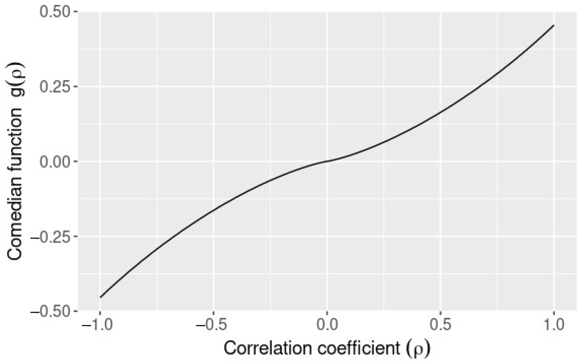
The univariate filter that is needed by the C3S-regression is implemented in the robreg3S package, while the GRE is computed using the GSE function with the option method = "rocke". Two versions of the C3S-regression to be considered are: (i) the full version using the comedian covariance matrix; and, (ii) the light version using the raw comedian matrix as an initial scatter estimate. The last one is called light version, because it uses less operations to compute than the full version. From now on, the C3S-regression is referred to both versions, unless that an indication is done.
Next, the regression model presented in Equation (
8) with
and
, 300, 500, 1000,
is considered. The values of covariates
, for
, are generated from a multivariate normal distribution
. We set
and
[
8], for
, without loss of generality, because the GSE used by the C3S-regression is location and scale equivariant. (Note that from the location equivariant of the GSE,
can be set.) To address the fact that the C3S-regression and 3S-regression are neither affine-equivariant nor regression equivariant, the correlation structure
may be used. Observe that this correlation structure is described in [
27], with the condition number fixed at 100 and random generation of
as
. Let
and
follow a uniform distribution on the unit spherical surface. The response variable
is given by
, where
, for
, are independent. The scenarios assumed in the simulation study are:
- S1
Clean data: the data generation is not altered.
- S2
Cell-wise contamination: randomly replace a proportion q of the cells in the covariates by outliers and of the responses by outliers , where .
- S3
Case-wise contamination: randomly replace a proportion
q of the cases by leverage outliers
, where
, and
, with
, for
. Here,
is the eigenvector corresponding to the smallest eigenvalue of
with length such that
. To compute the value of
, we follow the same process introduced in [
8,
27]; that is, a Monte Carlo study with the same number of replicates
. We observe that
is the value that produces the worst performance of the scatter estimator.
Let
for the cell-wise contamination. From the fact that case-wise outliers are unusual in practice, we consider
for the case-wise contamination. The number of replicates for each setting is
. In addition, the simulation study is also carried out in order to consider the regression model presented by Equation (
13) with
continuous covariates,
dummy covariates, and
. Then, the performance of the M-regression and C3S-regression is evaluated. The values of covariates
, for
, are first generated from a multivariate normal distribution
, where
is the randomly generated correlation matrix with a fixed condition number of 100. Subsequently,
is dichotomized at
, with
, for
, respectively. The generation of the model with continuous and dummy covariates follows the scenarios S1-S2 and for the case-wise contamination follows the scenario S3.
Let be a sub-matrix of , which quantifies the covariance of the continuous covariates. In this new scenario, randomly replace a proportion q of the cases in by leverage outliers , where , , with , and . Here, is now the eigenvector corresponding to the smallest eigenvalue of , with length such that , and the corresponding least favorable case-wise contamination size for the twelve continuous variables is .
Once again, we consider
for the cell-wise contamination and
for the case-wise contamination. The number of replicates for each setting is
. Furthermore, the simulation study is conducted for non-normal covariates to compare the performance of the C3S-regression, 3S-regression, 2S-regression and LS estimators. For the C3S-regression, the full and light versions of the proposed estimator are considered. The same regression model with
and
is used, but the covariates are generated from a non-normal distribution [
8]. The covariates
, for
, are first generated from a multivariate normal distribution with zero mean and covariance matrix
, which is,
, where, again,
is a randomly generated correlation matrix with a fix condition number of 100. Subsequently, the covariates are transformed by means of
We consider a distribution for
as:
, with
;
, with
;
, with
;
, with
; and Pareto
, with
. The scenarios that are evaluated in this simulation study are as S1. For the cell-wise contamination, we replace
by the proportion of cells in the covariates with outliers
, and by the proportion of responses with outliers
.
4.2. Simulation Results
The statistical performance in the estimation of regression coefficients due to the effect of cell-wise and case-wise outliers can be evaluated using the empirical mean squared error (MSE), defined as
where
is the estimate of
at the
ith Monte Carlo replicate.
Table 2 and
Table 3 report the
defined in Equation (
15) for
in all the settings with
. The results for
are omitted, because they are similar to
.
Figure 2 and
Figure 3 show curves of
for cell-wise and case-wise contamination in models with
continuous covariates and
.
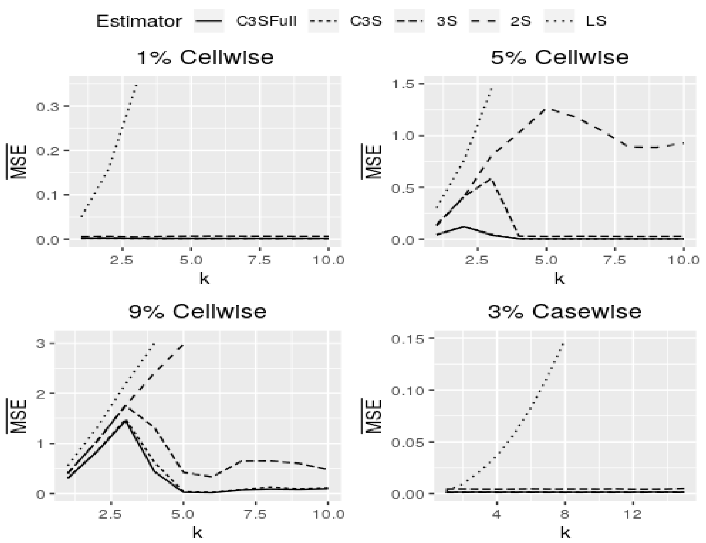
Figure 4 and
Figure 5 display curves of
for cell-wise and case-wise contamination in models with continuous and dummy covariates, and
.
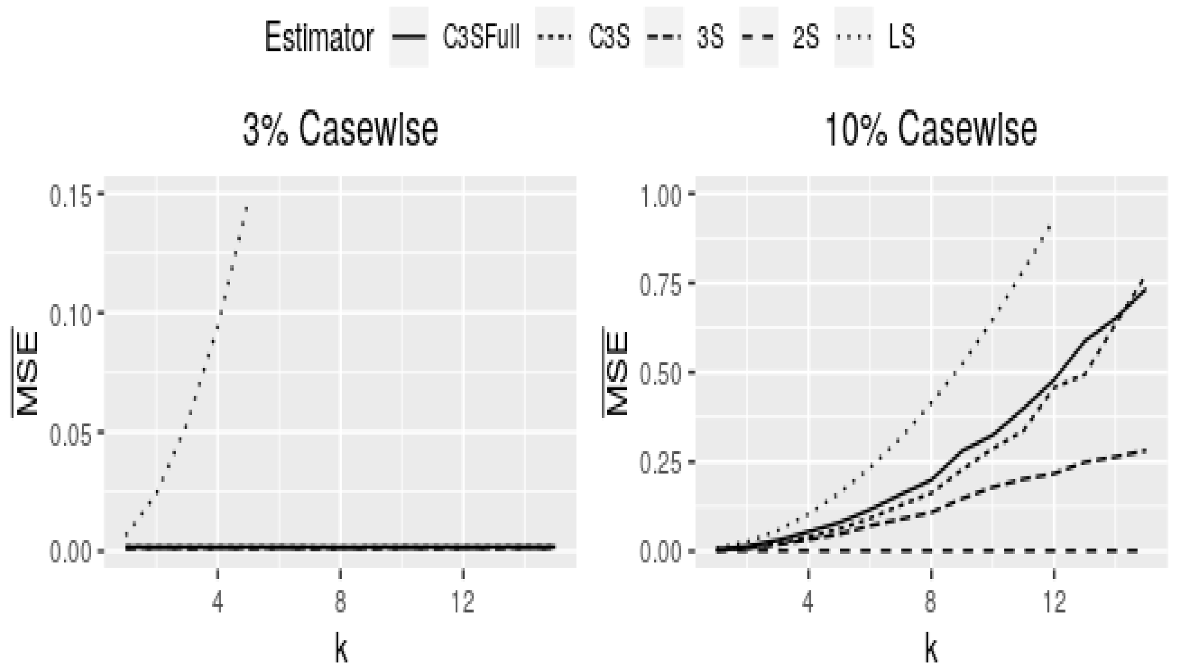
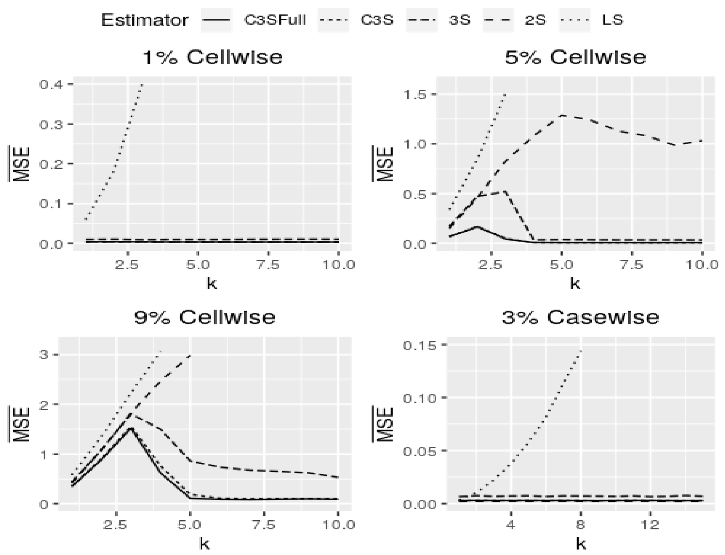
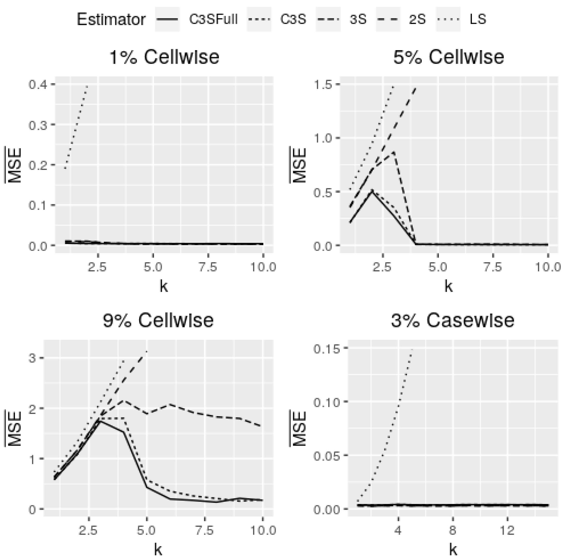
Figure 6 shows curves of
for cell-wise and case-wise contamination in models with continuous covariates and
. Note that models with continuous covariates in the M-regression and C3S-regression outperform in all of the assumed scenarios for both cell-wise and case-wise contaminations. In addition, in the four panels of
Figure 6, both versions of the C3S-regression have almost the same behavior for all settings assumed. The full version of the C3S-regression is little more robust than its light version, but the estimates of both are almost equal for all contamination settings. The results for
are similar to the cell-wise contamination settings. In the cell-wise contamination setting for small and moderate contamination proportions (
), the C3S-regression is highly robust against moderate and large cell-wise outliers (
), but less robust against inliers (
). The 3S-regression and C3S-regression perform similarly for moderate and large outliers, but in the presence of inliers (
), the 3S-regression is less robust; see first two panels of
Figure 6.
The 2S-regression and 3S-regression perform similarly in the presence of inliers, as expected from the simulation studies carried out in [
8]. However, the 2S-regression breaks down in cases when the proportion of contaminated cells is
; that is, when the propagation of large cell-wise outliers is expected to affect more than
of the cases.
For a large contamination proportion (), the C3S-regression, 3S-regression, and 2S-regression perform similarly in the presence of inliers (), but the 3S-regression breaks down for moderate and large cell-wise outliers (). However, the C3S-regression is highly robust against large cell-wise outliers () although less robust against moderate outliers. In the case-wise contamination setting, the C3S-regression, 3S-regression and 2S-regression perform fairly well and similarly. Nevertheless, the 2S-regression has the best performance, followed by the 3S-regression, which is followed in performance by the C3S-regression.
We also study the performance of the estimator with moderate and large case-wise contamination levels of and , in which at a size of leverage outliers of 22, the C3S-regression and 3S-regression break down as k increases. In this settings, the C3S-regression outperforms the 3S-regression, but, as expected, the 2S-regression maintains its robustness for any contamination level.
Note that, in practice, it is unusual to find case-wise outliers and even more at moderate or large levels. Thus, the loss of robustness for the C3S-regression and 3S-regression does not present a disadvantage. We detect that models with continuous and dummy covariates in the M-regression and C3S-regression outperform in all assumed scenarios.
Table 4 reports a summary of the performance of the estimators evaluated by
. The performance of the 3S-regression considering non-normal covariates is comparable to all the other estimators for clean data. However, both versions of the C3S-regression outperform all other estimators for any contamination size
k in the cell-wise contamination setting. In the cases of non-normal covariates, the C3S-regression maintains its competitive performance, followed by the 3S-regression, while the 2S-regression, as expected, breaks down in the presence of moderate and large cell-wise outliers proportion.
Next, the statistical performance of confidence intervals (CIs) for the regression coefficients based on the asymptotic covariance matrix, as described in Sub
Section 3.3, is evaluated. The asymptotic
CIs for the coefficients of C3S-regression can be established as
The performance of CIs defined in Equation (
16) may be evaluated using the empirical mean coverage rate (CR) given by
and the empirical mean CI length (CIL) defined as
Table 5 reports the average CIL defined in Equation (
18) obtained from the C3S-regression and 3S-regression in the case of clean data and contaminated data with
cell-wise (
),
cell-wise (
),
cell-wise (
) and
case-wise (
), for
. The results of the LS and 2S-regression estimates are not included here, because we are interested in comparing the CIL between the 3S-regression and C3S-regression. The CIL that is obtained from the C3S-regression is comparable to that of the 3S-regression for all considered scenarios. The CIL reached from the 3S-regression are shorter than that for the C3S-regression with clean data and data with small and moderate cell-wise contamination levels. For data with large cell-wise contamination levels or case-wise contamination, the CILs of the C3S-regression are shorter than the CILs of the 3S-regression. Moreover, for any assumed scenario, CILs of the 3S-regression and C3S-regression decrease as the sample size
n increases.
Figure 7 shows the
defined in Equation (
17) in the case of clean data and contaminated data with
cell-wise contamination (
), and
case-wise contamination (
), and for different sample sizes
. Although the results for the sample size
are not shown here for visualization, it can be noticed that, for the C3S-regression and 3S-regression, the evaluations of
under
are better than those when
. For contamination settings, the 3S-regression yields the best CR, which is the closest to the nominal level. In general, the CR for the C3S-regression is similar to that of the 3S-regression, and it tends to be equal as the sample size
n increases.
4.3. Analysis of Real Data
The airfoil self-noise data set is used for the illustration purpose. These data were obtained from a series of aerodynamic and acoustic tests of two and three-dimensional airfoil blade sections conducted in an anechoic wind tunnel by the NASA. The data set comprises airfoils of different sizes at various wind tunnel speeds and angles of attack with
observations (cases). For this data set,
Table 6 shows five covariates and one response variable along with their statistical summaries. This data set is available at the UCI repository [
42]. The aim of this empirical study is to predict the noise generated by an airfoil, from dimensions, speed and angle of attack. Specifically, the objective is to explain the scaled sound pressure level.
The data set is fitted with the model given by
where the log function is used for
due to its wide range and high skewness, while the log function is employed for
Y in order to improve the R2-adjusted. The corresponding parameters with C3S-regression (in both versions and full version computed by bootstrap estimation), 2S-regression, 3S-regression, and LS estimates are obtained. The regression coefficient estimates and the corresponding p-values are reported in
Table 7. Note that the regression coefficients are similar for all the estimates, except for the covariate
, (that is, the suction side displacement thickness). The coefficient of
estimated by 3S-regression and 2S-regression are similar, but are very different from the C3S-regression and LS estimates. For the C3S-regression,
is highly not significant, while for the 2S-regression and 3S-regression, it is only not significant. However, the LS method indicates that
is significant.
The squared norm distance, defined as
, is used to compare the four estimators.
Table 8 reports the corresponding SND, which shows that these distances from each two pairs are not large. Therefore, it suggests that the data are not contaminated or the contamination level is very small (inliers).


