Common Medical and Statistical Problems: The Dilemma of the Sample Size Calculation for Sensitivity and Specificity Estimation


Abstract
:1. Introduction
2. Materials and Methods
2.1. Interval Estimation Using Different Methods
2.2. New Expressions for Coverage Probability and Expected Length of a Conditional Probability Interval
2.3. Optimal and Approximate Sample Size Determination
3. Results
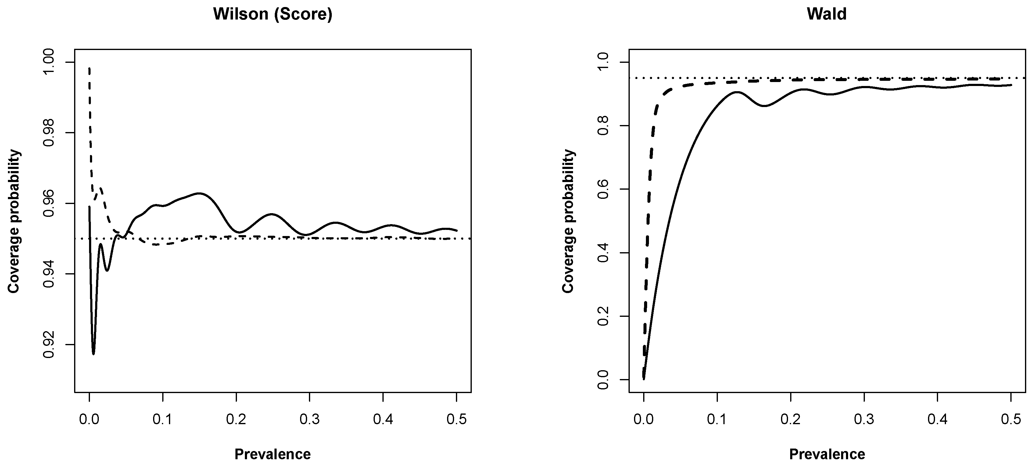
3.1. New Expressions for Coverage Probability of Interval Estimation Methods
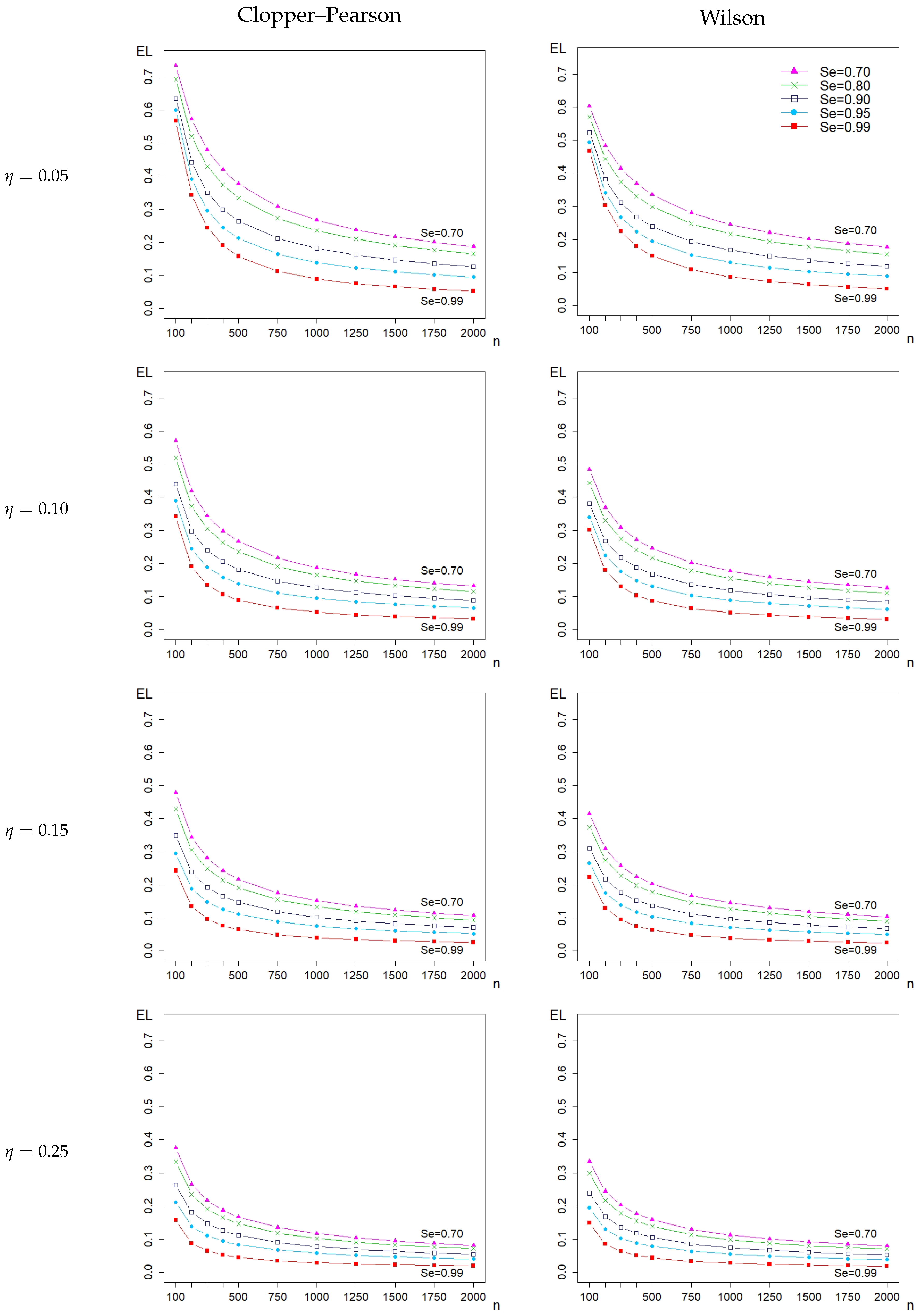
3.2. Impact on Sample Sizes
4. Discussion and Conclusions
Supplementary Materials
Author Contributions
Funding
Acknowledgments
Conflicts of Interest
Abbreviations
| CI | Confidence interval |
| CP | Coverage probability |
| EL | Expected length |
| Se | Sensitivity |
| Sp | Specificity |
Appendix A
Appendix B

| Method | R command |
| Clopper–Pearson | prop.ci() |
| Bayesian-U | prop.ci() |
| Jeffreys | prop.ci() |
| Agresti–Coull | prop.ci() |
| Wilson | prop.ci() |
| Wald | prop.ci() |
References
- Altman, D.; Machin, D.; Bryant, T.; Gardner, M. Statistics with Confidence. Confidence Intervals and Statistical Guidelines; BMJ: London, UK, 2000. [Google Scholar]
- Bossuyt, P.M.; Reitsma, J.B.; Bruns, D.; Gatsonis, C.A.; Glasziou, P.; Irwig, L.; Lijmer, J.G.; Moher, D.; Rennie, D.; de Vet, H.C.; et al. STARD 2015: An updated list of essential items for reporting diagnostic accuracy studies. Clin. Chem. 2015, h5527. [Google Scholar] [CrossRef] [Green Version]
- Korevaar, D.; Wang, J.; van Enst, W.A.; Leeflang, M.M.; Hooft, L.; Smidt, N.; Bossuyt, P.M.M. Reporting diagnostic accuracy studies: Some improvements after 10 years of STARD. Radiology 2015, 274, 781–789. [Google Scholar] [CrossRef] [PubMed]
- Newcombe, R. Two-sided confidence intervals for the single proportion: Comparison of seven methods. Stat. Med. 1998, 17, 857–872. [Google Scholar] [CrossRef]
- Agresti, A.; Coull, B. Approximate is better than “exact” for interval estimation of binomial proportions. Am. Stat. 1998, 52, 119–126. [Google Scholar]
- Brown, L.; Cai, T.; DasGupta, A. Interval estimation for a binomial proportion. Stat. Sci. 2001, 16, 101–117. [Google Scholar]
- Brown, L.; Cai, T.; Dasgupta, A. Confidence intervals for a Binomial proportion and asymptotic expansions. Ann. Stat. 2002, 30, 160–201. [Google Scholar]
- Pires, A.; Amado, C. Interval estimators for a binomial proportion: Comparison of twenty methods. REVSTAT J. 2008, 6, 165–197. [Google Scholar]
- Andrés, A.M.; Hernández, M.Á. Two-tailed asymptotic inferences for a proportion. J. Appl. Stat. 2014, 41, 1516–1529. [Google Scholar] [CrossRef]
- Zelmer, D.A. Estimating prevalence: A confidence game. J. Parasitol. 2013, 99, 386–389. [Google Scholar] [CrossRef] [PubMed]
- Gonçalves, L.; Oliveira, M.; Pascoal, C.; Pires, A. Sample size for estimating a binomial proportion: Comparison of different methods. Appl. Stat. 2012, 39, 2453–2473. [Google Scholar] [CrossRef]
- Flahault, A.; Cadilhac, M.; Thomas, G. Sample size calculation should be performed for design accuracy in diagnostic test studies. J. Clin. Epidemiol. 2005, 58, 859–862. [Google Scholar] [CrossRef] [PubMed]
- Amini, A.; Varsaneux, O.; Kelly, H.; Tang, W.; Chen, W.; Boeras, D.I.; Falconer, J.; Tucker, J.D.; Chou, R.; Ishizaki, A.; et al. Diagnostic accuracy of tests to detect hepatitis B surface antigen: A systematic review of the literature and meta-analysis. BMC Infect. Dis. 2017, 17, 698. [Google Scholar] [CrossRef] [PubMed]
- Thombs, B.D.; Rice, D.B. Sample sizes and precision of estimates of sensitivity and specificity from primary studies on the diagnostic accuracy of depression screening tools: A survey of recently published studies. Int. J. Methods Psychiat. Res. 2016, 25, 145–152. [Google Scholar] [CrossRef] [PubMed]
- R Core Team. R: A Language and Environment for Statistical Computing; R Foundation for Statistical Computing: Vienna, Austria, 2018. [Google Scholar]
- Sathish, N.; Vijayakumar, T.; Abraham, P.; Sridharan, G. Dengue fever: Its laboratory diagnosis, with special emphasis on IgM detection. Dengue Bull. 2003, 27, 116–125. [Google Scholar]
- Dendukuri, N.; Rahme, E.; Bélisle, P.; Joseph, L. Bayesian sample size determination for prevalence and diagnostic test studies in the absence of a gold standard test. Biometrics 2004, 60, 388–397. [Google Scholar] [CrossRef] [PubMed]
- Gonçalves, L.; Subtil, A.; Oliveira, M.; Rosário, V.; Lee, P.; Shaio, M.F. Bayesian latent class models in malaria diagnosis. PLoS ONE 2012, e40633. [Google Scholar] [CrossRef] [PubMed] [Green Version]
- Qiu, S.F.; Poon, W.Y.; Tang, M.L. Confidence intervals for proportion difference from two independent partially validated series. Stat. Methods Med. Res. 2016, 25, 2250–2273. [Google Scholar] [CrossRef] [PubMed]
- Gudbjartsson, D.F.; Helgason, A.; Jonsson, H.; Magnusson, O.T.; Melsted, P.; Norddahl, G.L.; Saemundsdottir, J.; Sigurdsson, A.; Sulem, P.; Agustsdottir, A.B.; et al. Spread of SARS-CoV-2 in the Icelandic population. N. Engl. J. Med. 2020. [Google Scholar] [CrossRef] [PubMed]
- Vos, P.; Hudson, S. Evaluation criteria for discrete confidence intervals: Beyond coverage and length. Am. Stat. 2005, 59, 137–142. [Google Scholar] [CrossRef]
- Newcombe, R. Measures of location for confidence intervals for proportions. Commun. Stat.-Theor. Methods 2011, 40, 1743–1767. [Google Scholar] [CrossRef]

| Clopper- | Anscombe | Agresti- | Bayesian | Jeffreys | Wilson | Wald | ||||||||
|---|---|---|---|---|---|---|---|---|---|---|---|---|---|---|
| Pearson | Coull | Uniform | ||||||||||||
| 0.75 | 11848 | −2 | 11855 | 5 | 11459 | −1 | 11449 | −11 | 11452 | 2 | 11538 | 78 | 11472 | 2 |
| 0.80 | 10165 | −45 | 10172 | −8 | 9869 | 39 | 9771 | 1 | 9847 | 37 | 9847 | 77 | 9864 | 54 |
| 0.85 | 8176 | −34 | 8184 | 4 | 7829 | −1 | 7852 | 22 | 7781 | −29 | 7853 | 23 | 7855 | 45 |
| 0.90 | 5880 | −10 | 5890 | 0 | 5589 | −21 | 5557 | 27 | 5488 | −2 | 5546 | 26 | 5532 | 12 |
| 0.91 | 5385 | 5 | 5395 | 5 | 5112 | 2 | 5024 | −26 | 5032 | 22 | 5031 | −19 | 5029 | 29 |
| 0.92 | 4877 | 7 | 4887 | −23 | 4626 | 6 | 4559 | 39 | 4521 | 31 | 4532 | 2 | 4514 | 14 |
| 0.93 | 4357 | 7 | 4368 | −22 | 4165 | 35 | 4045 | 35 | 3998 | 8 | 4024 | 4 | 3984 | 14 |
| 0.94 | 3824 | −16 | 3836 | 6 | 3638 | −2 | 3495 | 5 | 3463 | 33 | 3535 | 25 | 3441 | 11 |
| 0.95 | 3280 | 0 | 3293 | 3 | 3142 | 2 | 2991 | 21 | 2916 | 26 | 3008 | 28 | 2882 | 12 |
| 0.96 | 2723 | 3 | 2737 | 7 | 2653 | −7 | 2440 | 0 | 2341 | 1 | 2461 | 1 | 2302 | 12 |
| 0.97 | 2170 | 20 | 2185 | 15 | 2178 | −2 | 1915 | 5 | 1796 | 16 | 1944 | 4 | 1613 | −7 |
| 0.98 | 1584 | 4 | 1595 | 5 | 1722 | 2 | 1406 | 6 | 1272 | 12 | 1462 | 12 | 489 | 9 |
| 0.99 | 1079 | 9 | 1079 | 9 | 1284 | 14 | 931 | 11 | 913 | 13 | 1040 | 10 | NA | NA |
| Clopper- | Anscombe | Agresti- | Bayesian | Jeffreys | Wilson | Wald | ||||||||
|---|---|---|---|---|---|---|---|---|---|---|---|---|---|---|
| Pearson | Coull | Uniform | ||||||||||||
| 0.50 | 1741 | −2 | 1742 | −1 | 1696 | 0 | 1709 | 11 | 1697 | −1 | 1696 | 0 | 1700 | 0 |
| 0.55 | 1724 | −1 | 1738 | 12 | 1691 | 2 | 1685 | −4 | 1680 | 0 | 1685 | −4 | 1695 | 1 |
| 0.60 | 1673 | −1 | 1674 | −2 | 1628 | −1 | 1640 | 11 | 1629 | 0 | 1640 | 11 | 1632 | −2 |
| 0.65 | 1600 | 12 | 1601 | 12 | 1543 | −2 | 1543 | −2 | 1556 | 11 | 1543 | −2 | 1547 | 0 |
| 0.70 | 1469 | −1 | 1471 | 1 | 1428 | 2 | 1425 | −1 | 1436 | 10 | 1424 | −2 | 1433 | 1 |
| 0.75 | 1325 | 8 | 1317 | 0 | 1273 | −1 | 1275 | 1 | 1282 | 9 | 1281 | 7 | 1274 | −1 |
| 0.80 | 1130 | −5 | 1138 | 6 | 1093 | 0 | 1093 | 7 | 1093 | 3 | 1093 | 7 | 1095 | 5 |
| 0.85 | 908 | −5 | 915 | 6 | 870 | 0 | 865 | −5 | 865 | −3 | 871 | 1 | 870 | 2 |
| 0.90 | 657 | 2 | 654 | −1 | 621 | −3 | 616 | 1 | 610 | 0 | 617 | 3 | 614 | 0 |
| 0.91 | 602 | 4 | 603 | 4 | 571 | 3 | 561 | −1 | 558 | 1 | 559 | −3 | 558 | 2 |
| 0.92 | 545 | 3 | 546 | 0 | 514 | 0 | 502 | −1 | 498 | −1 | 503 | −1 | 500 | 0 |
| 0.93 | 484 | 0 | 485 | −3 | 462 | 3 | 446 | 0 | 443 | −1 | 447 | 0 | 442 | 0 |
| 0.94 | 425 | −2 | 426 | 0 | 405 | 0 | 390 | 2 | 384 | 2 | 392 | 2 | 381 | −1 |
| 0.95 | 366 | 1 | 366 | 0 | 349 | 0 | 331 | 1 | 323 | 1 | 333 | 1 | 319 | 0 |
| 0.96 | 304 | 1 | 305 | 1 | 294 | −2 | 271 | −1 | 260 | 0 | 274 | 0 | 254 | −1 |
| 0.97 | 240 | 1 | 241 | −1 | 242 | −1 | 213 | 0 | 198 | 0 | 216 | 0 | 179 | −1 |
| 0.98 | 176 | 0 | 177 | 0 | 191 | −1 | 156 | 0 | 140 | 0 | 161 | −1 | 54 | 0 |
| 0.99 | 119 | 0 | 119 | 0 | 142 | 0 | 103 | 0 | 100 | 0 | 114 | −1 | NA | NA |
| Interval Width () | ||||||||||||
|---|---|---|---|---|---|---|---|---|---|---|---|---|
| 0.05 | 0.06 | 0.07 | 0.08 | 0.09 | 0.10 | |||||||
| Clopper-Pearson | Wilson | Clopper-Pearson | Wilson | Clopper-Pearson | Wilson | Clopper-Pearson | Wilson | Clopper-Pearson | Wilson | Clopper-Pearson | Wilson | |
| 0.75 | 11,848 | 11,538 | 8280 | 7997 | 6119 | 5831 | 4711 | 4459 | 3742 | 3532 | 3046 | 2854 |
| 0.80 | 10,165 | 9847 | 7110 | 6826 | 5259 | 5006 | 4053 | 3825 | 3222 | 3003 | 2625 | 2428 |
| 0.85 | 8176 | 7853 | 5728 | 5445 | 4243 | 5445 | 3275 | 3995 | 2607 | 3054 | 2126 | 2399 |
| 0.90 | 5880 | 5546 | 4133 | 3838 | 3071 | 2839 | 2377 | 2165 | 1897 | 1719 | 1552 | 1389 |
| 0.91 | 5385 | 5031 | 3789 | 3523 | 2818 | 2578 | 2183 | 1987 | 1744 | 1567 | 1428 | 1272 |
| 0.92 | 4877 | 4532 | 3436 | 3158 | 2559 | 2340 | 1984 | 1797 | 1587 | 1419 | 1301 | 1158 |
| 0.93 | 4357 | 4024 | 3074 | 2808 | 2293 | 2074 | 1781 | 1604 | 1426 | 1270 | 1170 | 1036 |
| 0.94 | 3824 | 3535 | 2705 | 2454 | 2021 | 1827 | 1573 | 1404 | 1262 | 1121 | 1040 | 917 |
| 0.95 | 3280 | 3008 | 2326 | 2098 | 1743 | 1569 | 1360 | 1217 | 1094 | 976 | 905 | 801 |
| 0.96 | 2723 | 2461 | 1951 | 1742 | 1460 | 1307 | 1148 | 1028 | 925 | 829 | 768 | 691 |
| 0.97 | 2170 | 1944 | 1555 | 1403 | 1174 | 1064 | 930 | 849 | 763 | 697 | 639 | 586 |
| 0.98 | 1584 | 1462 | 1167 | 1080 | 903 | 845 | 732 | 686 | 613 | 576 | 525 | 494 |
| 0.99 | 1079 | 1040 | 833 | 807 | 679 | 659 | 571 | 554 | 491 | 476 | 431 | 417 |
| Interval Width () | ||||||||||||
|---|---|---|---|---|---|---|---|---|---|---|---|---|
| 0.05 | 0.06 | 0.07 | 0.08 | 0.09 | 0.10 | |||||||
| Clopper-Pearson | Wilson | Clopper-Pearson | Wilson | Clopper-Pearson | Wilson | Clopper-Pearson | Wilson | Clopper-Pearson | Wilson | Clopper-Pearson | Wilson | |
| 0.50 | 1741 | 1696 | 1222 | 1184 | 901 | 864 | 692 | 663 | 547 | 521 | 445 | 421 |
| 0.55 | 1724 | 1685 | 1203 | 1172 | 888 | 855 | 683 | 656 | 542 | 517 | 440 | 418 |
| 0.60 | 1673 | 1640 | 1171 | 1130 | 862 | 833 | 665 | 636 | 527 | 500 | 428 | 405 |
| 0.65 | 1600 | 1543 | 1115 | 1077 | 822 | 786 | 630 | 601 | 501 | 474 | 406 | 384 |
| 0.70 | 1469 | 1424 | 1028 | 988 | 760 | 726 | 583 | 556 | 464 | 437 | 377 | 354 |
| 0.75 | 1325 | 1281 | 925 | 887 | 680 | 650 | 523 | 497 | 416 | 391 | 339 | 316 |
| 0.80 | 1130 | 1093 | 790 | 753 | 586 | 553 | 450 | 424 | 358 | 334 | 291 | 270 |
| 0.85 | 908 | 871 | 636 | 604 | 471 | 443 | 364 | 338 | 289 | 267 | 236 | 215 |
| 0.90 | 657 | 617 | 459 | 426 | 342 | 314 | 264 | 240 | 211 | 190 | 172 | 154 |
| 0.91 | 602 | 559 | 421 | 390 | 313 | 286 | 242 | 220 | 193 | 174 | 158 | 141 |
| 0.92 | 545 | 503 | 383 | 351 | 284 | 259 | 220 | 199 | 176 | 157 | 144 | 128 |
| 0.93 | 484 | 447 | 341 | 313 | 255 | 231 | 198 | 177 | 158 | 141 | 130 | 115 |
| 0.94 | 425 | 392 | 301 | 273 | 225 | 202 | 174 | 156 | 140 | 124 | 115 | 101 |
| 0.95 | 366 | 333 | 258 | 233 | 193 | 173 | 151 | 134 | 121 | 108 | 100 | 88 |
| 0.96 | 304 | 274 | 216 | 194 | 162 | 145 | 127 | 113 | 102 | 92 | 85 | 76 |
| 0.97 | 240 | 216 | 172 | 155 | 130 | 118 | 103 | 93 | 84 | 77 | 70 | 64 |
| 0.98 | 176 | 161 | 129 | 119 | 100 | 93 | 81 | 76 | 67 | 63 | 57 | 54 |
| 0.99 | 119 | 114 | 92 | 89 | 75 | 72 | 63 | 61 | 54 | 52 | 47 | 45 |
© 2020 by the authors. Licensee MDPI, Basel, Switzerland. This article is an open access article distributed under the terms and conditions of the Creative Commons Attribution (CC BY) license (http://creativecommons.org/licenses/by/4.0/).
Share and Cite
Oliveira, M.R.; Subtil, A.; Gonçalves, L. Common Medical and Statistical Problems: The Dilemma of the Sample Size Calculation for Sensitivity and Specificity Estimation. Mathematics 2020, 8, 1258. https://doi.org/10.3390/math8081258
Oliveira MR, Subtil A, Gonçalves L. Common Medical and Statistical Problems: The Dilemma of the Sample Size Calculation for Sensitivity and Specificity Estimation. Mathematics. 2020; 8(8):1258. https://doi.org/10.3390/math8081258
Chicago/Turabian StyleOliveira, M. Rosário, Ana Subtil, and Luzia Gonçalves. 2020. "Common Medical and Statistical Problems: The Dilemma of the Sample Size Calculation for Sensitivity and Specificity Estimation" Mathematics 8, no. 8: 1258. https://doi.org/10.3390/math8081258
APA StyleOliveira, M. R., Subtil, A., & Gonçalves, L. (2020). Common Medical and Statistical Problems: The Dilemma of the Sample Size Calculation for Sensitivity and Specificity Estimation. Mathematics, 8(8), 1258. https://doi.org/10.3390/math8081258