Definition and Estimation of Covariate Effect Types in the Context of Treatment Effectiveness

Abstract

In some clinical studies, assessing covariate effect types indicating whether a covariate is predictive and/or prognostic is of interest, in addition to the study endpoint. Recently, for a case with a binary outcome, Chiba (Clinical Trials, 2019; 16: 237–245) proposed the new concept of covariate effect type, which is assessed in terms of four response types, and showed that standard subgroup or regression analysis is applicable only in certain cases. Although this concept could be useful for supplementing conventional standard analysis, its application is limited to cases with a binary outcome. In this article, we aim to generalize Chiba’s concept to continuous and time-to-event outcomes. We define covariate effect types based on four response types. It is difficult to estimate the response types from the observed data without making certain assumptions, so we propose a simple method to estimate them under the assumption of independent potential outcomes. Our approach is illustrated using data from a clinical study with a time-to-event outcome.

1. Introduction

In certain clinical studies, it is important to assess covariate effect types to indicate whether a covariate is predictive and/or prognostic in the context of treatment effectiveness. Clark et al. [1] defined a predictive factor as a factor associated with the response or lack of response to a particular therapy, while a prognostic factor is a factor associated with the clinical outcome in the absence of therapy, or with the application of a standard therapy. To assess whether a covariate is predictive and/or prognostic, subgroup or regression analysis is often used [2]. For a case with a binary outcome, on the difference scale, a binary covariate $Z$ is predictive if

$$\delta \equiv \left\{\mathrm{Pr}\left(Y=1|X=1, Z=1\right)-\mathrm{Pr}\left(Y=1|X=0, Z=1\right)\right\}-\left\{\mathrm{Pr}\left(Y=1|X=1, Z=0\right)-\mathrm{Pr}\left(Y=1|X=0, Z=0\right)\right\}$$

(1)

is not zero, where $X$ is the treatment arm ($X=1$ for the experimental treatment and $X=0$ for the control treatment) and $Y$ is the outcome ($Y=1$ for response and $Y=0$ for no response). If $\delta$ is close to zero, $Z$ is prognostic if

$$\gamma \equiv \mathrm{Pr}\left(Y=1|X=0, Z=1\right)-\mathrm{Pr}\left(Y=1|X=0, Z=0\right)$$

(2)

is not zero.

Recently, for cases with a binary outcome, Chiba [3] proposed assessing covariate effect types based on four response types [4] defined in terms of the potential outcome of $Y$ if $X$ is $x$, $Y\left(x\right)$, rather than $\delta$ and $\gamma$ as above. The four response types are defined as follows:

• Activated subjects, who would show a response regardless of the treatment they received; that is, $\left\{Y\left(1\right), Y\left(0\right)\right\}=\left(1, 1\right)$;
• Causative subjects, who would show a response only if they received the experimental treatment; that is, $\left\{Y\left(1\right), Y\left(0\right)\right\}=\left(1, 0\right)$;
• Preventive subjects, who would show a response only if they received the control treatment; that is, $\left\{Y\left(1\right), Y\left(0\right)\right\}=\left(0, 1\right)$;
• Inert subjects, who would not show a response regardless of the treatment they received; that is, $\left\{Y\left(1\right), Y\left(0\right)\right\}=\left(0, 0\right)$.

Based on the four response types, measures of the covariate effect types are defined as follows [3]:

$${\eta }_{kl}\equiv \mathrm{Pr}\left\{Y\left(1\right)=k, Y\left(0\right)=l|Z=1\right\}-\mathrm{Pr}\left\{Y\left(1\right)=k, Y\left(0\right)=l|Z=0\right\}$$

(3)

for $k, l=0, 1$. Then, ${\eta }_{10}$ can be used instead of a current common measure for predicting the effectiveness of the experimental treatment, i.e., $\delta$ in (1). ${\eta }_{10}>0$ indicates that the proportion of subjects who would show a response only if they received the experimental treatment is higher in the subgroup where $Z=1$ than in the subgroup where $Z=0$. In addition, we can consider predictability for the effectiveness of the control treatment (or the harm caused by the experimental treatment) by ${\eta }_{01}$. Instead of a current common measure for a prognostic factor, i.e., $\gamma$ in (2), ${\eta }_{11}$ can be used. ${\eta }_{11}>0$ indicates that the proportion of subjects who would show a response regardless of the treatment they received is higher in the subgroup where $Z=1$ than in the subgroup where $Z=0$.

Applying the potential outcome $Y\left(x\right)$ to (1) under the assumption of $Y\left(x\right)\perp X|Z$, which indicates that $Y\left(x\right)$ is independent from $X$ given $Z$, the following relationship between (1) and (3) is obtained:

$$\begin{array}{cc}\hfill \delta & =\left[\mathrm{Pr}\left\{Y\left(1\right)=1|Z=1\right\}-\mathrm{Pr}\left\{Y\left(0\right)=1|Z=1\right\}\right]-\left[\mathrm{Pr}\left\{Y\left(1\right)=1|Z=0\right\}-\mathrm{Pr}\left\{Y\left(0\right)=1|Z=\right\}\right]\hfill \\ & ={\eta }_{10}-{\eta }_{01}.\hfill \end{array}$$

(4)

Similarly, the following relationship holds between (2) and (3):

$$\begin{array}{cc}\hfill \gamma & =\mathrm{Pr}\left\{Y\left(0\right)=1|Z=1\right\}-\mathrm{Pr}\left\{Y\left(0\right)=1|Z=0\right\}\hfill \\ & ={\eta }_{11}+{\eta }_{01}.\hfill \end{array}$$

(5)

Obviously, if ${\eta }_{01}\ne 0$, the currently used definition of covariate effect types does not correspond to the new definition in (3). Except for the special case of ${\eta }_{01}=0$, under the current definition, the two characteristics of covariate effect cannot be separated from each other. In actual clinical studies, the aim is to assess covariate effect type on the basis of (3) rather than (1) and (2). However, (3) can be applied only when an outcome is binary and not when an outcome is continuous or time-to-event-based. In this article, we aim to generalize (3) to continuous and time-to-event outcomes. We provide a definition of measures of covariate effect types in Section 2 and propose a simple method to estimate those measures in Section 3. In Section 4, our approach is illustrated using data from a clinical study with a time-to-event outcome. Finally, in Section 5, the performance of the proposed approach and directions for future work in this area are discussed.

2. Definition of Measures of Covariate Effect Types

In the following, we mainly discuss a case with a time-to-event outcome $T$. However, this discussion can also be applied to a case with a continuous outcome as a special case without censored data in which a larger value represents a better response. $X$ and $Z$ are the same as in Section 1; i.e., $X$ is a binary treatment arm and $Z$ is a binary covariate. $T\left(x\right)$ is the potential outcome of $T$ if $X$ had been set to $x$. Unfortunately, it is not possible to observe the values of both $T\left(1\right)$ and $T\left(0\right)$; i.e., $T=T\left(1\right)X+T\left(0\right)\left(1-X\right)$ [5]. We use the stable unit treatment value assumption under which a single version of each treatment is available and there is no interference among subjects [6,7].

When an outcome is time-to-event, the response type $\left\{T\left(1\right), T\left(0\right)\right\}$ cannot be classified into four types unlike in the case of a binary outcome described in Section 1. However, if we set a cut-off point $t_c$, the time-to-event outcome can be regarded as a binary variable; then, we can consider the following four response types.

Definition 1 

(Response type).Using a cut-off point$t_c$, the response type can be classified into the following four types:

• Activated subjects (type 11 subjects), whose outcomes would be larger than or equal to$t_c$, regardless of the treatment they received; that is,$\left\{T\left(1\right)\ge t_c, T\left(0\right)\ge t_c\right\}$;
• Causative subjects (type 10 subjects), whose outcomes would be larger than or equal to$t_c$if they received the experimental treatment, but would be smaller than$t_c$if they received the control treatment; that is,$\left\{T\left(1\right)\ge t_c, T\left(0\right)<t_c\right\}$;
• Preventive subjects (type 01 subjects), whose outcomes would be smaller than$t_c$if they received the experimental treatment, but would be larger or equal to$t_c$if they received the control treatment; that is,$\left\{T\left(1\right)<t_c, T\left(0\right)\ge t_c\right\}$;
• Inert subjects (type 00 subjects), whose outcomes would be smaller than$t_c$, regardless of the treatment they received; that is,$\left\{T\left(1\right)<t_c, T\left(0\right)<t_c\right\}$.

All subjects belong to one of these four types, although we cannot know which type a subject belongs to. We denote a proportion of the $kl$ subjects of the total subjects as $P_{kl}\left(t_c\right)$; i.e.,

$$P_{kl}\left(t_c\right)\equiv {\left[\mathrm{Pr}\left\{T\left(1\right)\ge t_c, T\left(0\right)\ge t_c\right\}\right]}^{kl}{\left[\mathrm{Pr}\left\{T\left(1\right)\ge t_c, T\left(0\right)<t_c\right\}\right]}^{k\left(1-l\right)}\times {\left[\mathrm{Pr}\left\{T\left(1\right)<t_c, T\left(0\right)\ge t_c\right\}\right]}^{\left(1-k\right)l}{\left[\mathrm{Pr}\left\{T\left(1\right)<t_c, T\left(0\right)<t_c\right\}\right]}^{\left(1-k\right)\left(1-l\right)},$$

(6)

and the proportion in the stratum with $Z=z$ as $P_{kl,z}\left(t_c\right)$. Then, $P_{11}\left(t\right)+P_{10}\left(t\right)=\mathrm{Pr}\left\{T\left(1\right)\ge t\right\}$ corresponds to the survival probability under the experimental condition and $P_{11}\left(t\right)+P_{01}\left(t\right)=\mathrm{Pr}\left\{Y\left(0\right)\ge t\right\}$ is that under the control condition. For a continuous outcome, they correspond to one minus the cumulative density function.

Using $P_{kl,z}\left(t_c\right)$, we can simply define measures of covariate effect types at the cut-off point $t_c$ by

$${\theta }_{kl}\left(t_c\right)\equiv P_{kl,1}\left(t_c\right)-P_{kl,0}\left(t_c\right).$$

(7)

This is essentially the same as ${\eta }_{kl}$ in (3). Unfortunately, ${\theta }_{kl}\left(t_c\right)$ with a fixed $t_c$ cannot be applied as a general definition of measures of covariate types. If there is a medically meaningful cut-off point, the outcome is no longer time-to-event (continuous); rather, it is binary. If the cut-off point $t_c$ has no medical significance, it is not valuable to use a fixed cut-off point. $P_{kl}\left(t_c\right)$ and $P_{kl,z}\left(t_c\right)$ with a fixed cut-off point $t_c$ may also not be useful. Using these probabilities with $t_c$ changed on the interval, we define the restricted mean probability (RMP) as follows.

Definition 2 

(Restricted mean probability).The restricted mean probability for response type on the interval$\left[t_a, t_b\right]$,${\overline{P}}_{kl}$, is defined by the following formula:

$${\overline{P}}_{kl}\equiv \frac{1}{t_b-t_a}{{\displaystyle \int }}_{t_a}^{t_b}{P}_{kl}\left(t_c\right)d{t}_c$$

for$k, l=0, 1$.

In this definition, $t_a$ and $t_b$ will usually be set to $t_a=0$ and $t_b=t_{\tau }$, respectively, where $t_{\tau }$ is the truncation time; for a continuous outcome, these values will be set to the minimum and maximum values of the observed outcome, respectively. ${\overline{P}}_{kl,z}$ in the stratum with $Z=z$ is defined in the same manner. ${\overline{P}}_{kl}$ is the restricted expectation of $P_{kl}\left(t_c\right)$ on the interval $\left[t_a, t_b\right]$. Then, ${\overline{P}}_{kl}$ is interpreted as the mean proportion of type $kl$ subjects when the cut-off point is changed from $t_a$ to $t_b$.

It is important to note that ${\overline{P}}_{kl}$ is related to $\mathrm{E}\left[\min \left\{\max \left\{T\left(x\right), t_a\right\}, t_b\right\}\right]$, which is the restricted expectation of the potential outcome $T\left(x\right)$ on the interval $\left[t_a, t_b\right]$.

Lemma 1. 

We have the following relationships between${\overline{P}}_{kl}$and$\mathrm{E}\left[\min \left\{\max \left\{T\left(x\right), t_a\right\}, t_b\right\}\right]$:

$$\begin{gathered} \mathrm{E}\left[\min \left\{\max \left\{T\left(1\right), t_a\right\}, t_b\right\}\right]=\left(t_b-t_a\right)\left({\overline{P}}_{11}+{\overline{P}}_{10}\right)+t_a, \\ \mathrm{E}\left[\min \left\{\max \left\{T\left(0\right), t_a\right\}, t_b\right\}\right]=\left(t_b-t_a\right)\left({\overline{P}}_{11}+{\overline{P}}_{01}\right)+t_a. \end{gathered}$$

The proof is given in Appendix A. The difference between these two equations indicates that the restricted average causal effect on the interval $\left[t_a, t_b\right]$ can be expressed as $\left(t_b-t_a\right)\left({\overline{P}}_{10}-{\overline{P}}_{01}\right)$. Notably, when $t_a=0$ and $t_b=t_{\tau }$, $t_{\tau }\left({\overline{P}}_{11}+{\overline{P}}_{10}\right)$ and $t_{\tau }\left({\overline{P}}_{11}+{\overline{P}}_{01}\right)$ correspond to the restricted mean survival times (RMSTs) [8,9,10], which are equal to the areas under the survival curves on the interval $\left[0,t_{\tau }\right]$ under the experimental and control conditions, respectively. Similarly, $t_{\tau }\left({\overline{P}}_{01}+{\overline{P}}_{00}\right)$ and $t_{\tau }\left({\overline{P}}_{10}+{\overline{P}}_{00}\right)$ correspond to the restricted mean time lost [9] under the experimental and control conditions, respectively.

We give a general definition of measures of covariate effect types using ${\overline{P}}_{kl,z}$, which is the RMP of a given response type in the stratum with $Z=z$.

Proposition 1. 

We define a measure of covariate effect type as${\overline{\theta }}_{kl}\equiv {\overline{P}}_{kl,1}-{\overline{P}}_{kl,0}$for$k, l=0, 1$.

The interpretation of ${\overline{\theta }}_{kl}$ is similar to that of ${\eta }_{kl}$ in (3) for a case with a binary outcome. As a prediction measure, we use ${\overline{\theta }}_{10}$ and ${\overline{\theta }}_{01}$. ${\overline{\theta }}_{10}>0$ implies the subgroup where $Z=1$ contains a higher proportion of subjects who would survive longer by receiving the experimental treatment than the subgroup where $Z=0$. Then, $Z$ predicts the effectiveness of the experimental treatment, and we say that $Z$ is “augmented-causative”. If ${\overline{\theta }}_{10}<0$, we say that $Z$ is “depleted-causative”. In a similar sense, ${\overline{\theta }}_{01}$ is a prediction measure of the effectiveness of the control treatment (or for the harm associated with proceeding with the experimental treatment).

We note that for a case with a time-to-event (continuous) outcome, we can obtain results similar to (4) and (5) when the outcome is binary. Using Proposition 1 and Lemma 1, the prediction and prognosis measures based on conventional standard analysis, ${\delta }^{\prime }$ and ${\gamma }^{\prime }$, can be expressed as functions of ${\overline{\theta }}_{kl}$ on the difference scale.

Corollary 1. 

We have the following equations:

$$\begin{gathered} {\delta }^{\prime }\equiv \left(E_{1,1}-E_{0,1}\right)-\left(E_{1,0}-E_{0,0}\right)=\left(t_b-t_a\right)\left({\overline{\theta }}_{10}-{\overline{\theta }}_{01}\right), \\ {\gamma }^{\prime }\equiv E_{0,1}-E_{0,0}=\left(t_b-t_a\right)\left({\overline{\theta }}_{11}+{\overline{\theta }}_{01}\right), \end{gathered}$$

where$E_{x,z}\equiv \mathrm{E}\left[\min \left\{\max \left\{T\left(x\right), t_a\right\}, t_b\right\}|Z=z\right]$.

On the basis of this corollary, ${\overline{\theta }}_{11}$ in Proposition 1 can be related to the prognosis under the current standard analysis. Similar to the currently used standard analysis, if ${\overline{\theta }}_{10}$ is close to ${\overline{\theta }}_{01}$, which implies that ${\delta }^{\prime }$ is close to zero, $Z$ is prognostic if ${\overline{\theta }}_{11}$ is not zero. ${\overline{\theta }}_{11}>0$ implies that the mean survival time is longer for subjects in the subgroup where $Z=1$ than the subgroup where $Z=0$, regardless of the treatment they received. In this case, we say that $Z$ is “augmented-activated”. In contrast, when ${\overline{\theta }}_{11}<0$, we say that $Z$ is “depleted-activated”.

Finally, we emphasize that Corollary 1 indicates that the results of the current standard analysis can be properly interpreted when ${\overline{\theta }}_{01}=0$; however, this may not be the case when ${\overline{\theta }}_{01}\ne 0$. On the other hand, our measure of covariate effect type can assess whether a covariate is predictive and/or prognostic, even when ${\overline{\theta }}_{01}\ne 0$.

3. Estimation of Measures of Covariate Effect Types

Unfortunately, ${\overline{\theta }}_{kl}$ in Proposition 1 cannot be identified based on the observed data without making certain assumptions, because the joint probability of $Y\left(1\right)$ and $Y\left(0\right)$ cannot be estimated [11,12]. Therefore, we use two assumptions that are often applied in the context of the pairwise comparison based on $\mathrm{Pr}\{T\left(x\right)>T\left(1-x\right)\}$ [13,14,15].

Assumption 1 

(Ignorable treatment assignment).The potential outcome$T\left(x\right)$is independent of the treatment arm$X$; i.e.,$T\left(x\right)\perp X$. It is also assumed that$T\left(x\right)\perp X|Z$.

Assumption 2 

(Independent potential outcome).Two potential outcomes are independent of each other; i.e.,$T\left(1\right)\perp T\left(0\right)$.

Assumption 1 is often made in randomized trials. Although some authors have discussed methods to infer $\mathrm{Pr}\{T\left(x\right)>T\left(1-x\right)\}$ without Assumption 2 [16,17], the methods are impractical as they tend to be complex and/or require considerable computational effort.

Corollary 2. 

$P_{kl}\left(t_c\right)$ in (6) is identified under Assumptions 1 and 2 as follows:

$$P_{kl}\left(t_c\right)={\left[\mathrm{Pr}\{T\ge t_c|X=1\}\right]}^k{\left[\mathrm{Pr}\left\{T⟨t_c|X=1\right\}\right]}^{1-k}\times {\left[\mathrm{Pr}\{T\ge t_c|X=0\}\right]}^l{\left[\mathrm{Pr}\left\{T⟨t_c|X=0\right\}\right]}^{1-l}.$$

$P_{kl,z}\left(t_c\right)$ in the stratum with $Z=z$ is also identified under Assumptions 1 and 2, thus allowing ${\overline{P}}_{kl,z}$ in Definition 2 and ${\overline{\theta }}_{kl}$ in Proposition 1 to be identified.

We propose a method to estimate ${\overline{P}}_{kl}$ in Definition 2 based on the formula in Corollary 2. Let us denote the observed event occurrence or censoring time as $t_1<\cdots <t_j<\cdots <t_D$ in which the time points in both arms are included. Then, we can use the cut-off point $t_c$ as a discrete value taking only the same value as $t_j$; that is, it is sufficient to consider $t_1, \dots , t_D$ as the cut-off points. We also set the interval $\left[t_a, t_b\right]$ to $\left[0, t_{\tau }\right]$, where $t_{\tau } (\le t_D)$ is the truncation time. These settings yield the following formula to estimate ${\overline{P}}_{kl}$.

Proposition 2. 

For a time-to-event outcome, we estimate$P_{kl,z}\left(t_c\right)$with truncation time$t_{\tau }$under Assumptions 1 and 2 as follows:

$${\widehat{P}}_{kl}\left(t_c\right)={\left\{{\widehat{S}}_1\left(t_{c-1}\right)\right\}}^k{\left\{1-{\widehat{S}}_1\left(t_{c-1}\right)\right\}}^{1-k}{\left\{{\widehat{S}}_0\left(t_{c-1}\right)\right\}}^l{\left\{1-{\widehat{S}}_0\left(t_{c-1}\right)\right\}}^{1-l},$$

where$t_0=0$and$S_x\left(t_{c-1}\right)\equiv \mathrm{Pr}\{T\ge t_c|X=x\}$ is the survival probability estimated using the Kaplan–Meier method. Then, we estimate ${\overline{P}}_{kl}$ by

$${\widehat{\overline{P}}}_{kl}=\frac{1}{\tau }{\displaystyle \sum }_{c=1}^{\tau }\left(t_c-t_{c-1}\right){\widehat{P}}_{kl}\left(t_c\right).$$

Censoring is considered when estimating $S_x(t_{c-l}$ by the Kaplan–Meier method. In a similar manner, $P_{kl,z}\left(t_c\right)$ and ${\overline{P}}_{kl,z}$ are estimated by applying Proposition 2 to the stratum with Z = z. Thus, ${\theta }_{kl,z}\left(t_c\right)$, in (7) and ${\theta }_{kl,z}$ in Proposition 1 can be estimated based on the observed data. It is obvious from Proposition 2 that $\tau ({\widehat{\overline{P}}}_{11}+{\widehat{\overline{P}}}_{10})$ and $\tau ({\widehat{\overline{P}}}_{11}+{\widehat{\overline{P}}}_{01})$ are consistent with the estimators of the RMST in the arm with X = x.

To derive the formulas to estimate $P_{kl}\left(t_c\right)$ and ${\overline{P}}_{kl}$ for a continuous outcome without censoring, let us suppose that t₁ < ⋯ < t_j < ⋯ t_D are the observed values of the continuous outcome. The interval [t_a,t_b] is set to [t₁,t_D]. Here, we denote the number of subjects taking the value t_j in the experimental arm as n_j and that in the control arm as m_j. Then, $P_{kl}\left(t_j\right)$ and ${\overline{P}}_{kl}$ are estimated by the following formulas.

Proposition 3. 

For a continuous outcome, we estimate$P_{kl}\left(t_c\right) and {\overline{P}}_{kl}$ under Assumptions 1 and 2 by

$$\begin{gathered} {\widehat{P}}_{kl}\left(t_c\right)={\left(\frac{{{\displaystyle \sum }}_{j\ge c}{n}_j}{n}\right)}^k{\left(\frac{{{\displaystyle \sum }}_{j\le c-1}{n}_j}{n}\right)}^{1-k}{\left(\frac{{{\displaystyle \sum }}_{j\ge c}{m}_j}{m}\right)}^l{\left(\frac{{{\displaystyle \sum }}_{j\le c-1}{m}_j}{m}\right)}^{1-l}, \\ {\widehat{\overline{P}}}_{kl}=\frac{1}{t_D-t_1}{\displaystyle \sum }_{c=2}^D\left(t_c-t_{c-1}\right){\widehat{P}}_{kl}\left(t_c\right), \end{gathered}$$

where $n={{\displaystyle \sum }}_{j=1}^D{n}_j$ and $m={{\displaystyle \sum }}_{j=1}^D{m}_j$.

Let us denote the outcome values as $t_{j_1}^1$ ($j_1=1, \dots , D_1$) for subjects in the experimental arm and $t_{j_0}^0(j_0=1, \dots , D_0)$ for those in the control arm. Then, in relation to Lemma 1, we have Lemma 2 below.

Lemma 2. 

When${\widehat{P}}_{kl}\left(t_c\right) and {\widehat{\overline{P}}}_{kl}$ in Proposition 3 are used, the following equations hold:

$$\begin{gathered} \left(t_D-t_1\right)\left({\widehat{\overline{P}}}_{11}+{\widehat{\overline{P}}}_{10}\right)+t_1=\frac{1}{n}{\displaystyle \sum }_{j_1=1}^{D_1}{n}_{j_1}{t}_{j_1}^1, \\ \left(t_D-t_1\right)\left({\widehat{\overline{P}}}_{11}+{\widehat{\overline{P}}}_{01}\right)+t_1=\frac{1}{m}{\displaystyle \sum }_{j_0=1}^{D_0}{m}_{j_0}{t}_{j_0}^0. \end{gathered}$$

The proof is given in Appendix B. In this lemma, the right sides correspond to the arithmetic means in the arm with $X=x$. As the arithmetic mean is a plausible estimate of E{T|X = x}, the left sides are plausible estimates of unrestricted rather than restricted expectation of $T\left(x\right)$, $\mathrm{E}\left\{T\left(x\right)\right\}$, under Assumption 1.

4. Illustration

We illustrate our measure of covariate effect type using the clinical data set of Ohashi and Hamada [18]. The purpose of that study was to determine whether the survival time is longer with use of radiation during surgery ($X=1$) than without it ($X=0$) in subjects with pancreatic cancer. As it was an observational study, Assumption 1 would not hold. Nevertheless, we analyzed the data under this assumption, so the following analyses are for illustrative purposes only.

We explored the covariate effect type in the context of radiation effectiveness in the pancreatic cancer site, which was subclassified as pancreatic head ($Z=1$) or “other” ($Z=0$). In the pancreatic head subgroup, 51 subjects received radiation during surgery and 14 subjects did not. In the other subgroup, nine subjects (including one censored subject) received radiation and nine did not. The survival curves in both subgroups are shown in Figure 1. Table 1 summarizes the RMST estimates and differences between arms in both subgroups, with 95% confidence intervals (CIs). For the estimation, the truncation time was set to the maximum observed time, 21.6 (months), because the final survival probability was zero in both arms in both subgroups.

Figure 1. Survival curves for the arms with and without radiation during surgery: (a) pancreatic head subgroup; (b) “other” subgroup.

Table 1. Restricted mean survival times (RMSTs) for the arms with and without radiation, for the pancreatic head and “other” subgroups, and the RMST differences between the two arms.

Subgroup	Arm	RMST	RMST Difference (95% CI 1)
Pancreatic head	Radiation	5.508	1.236 (–1.127, 3.600)
	No radiation	4.271
Other	Radiation	9.963	5.585 (1.947, 9.223)
	No radiation	4.378

¹ Confidence intervals (CIs) were derived based on a normal approximation.

Before applying our approach, we first applied the current standard analysis given by ${\delta }^{\prime }$ and ${\gamma }^{\prime }$ in Corollary 1. Using the RMST estimates in Table 1, ${\widehat{\delta }}^{\prime }=-4.349$ (95% CI: –8.687, –0.011) and ${\widehat{\gamma }}^{\prime }=-0.106$ (95% CI: –2.635, 2.422). As ${\widehat{\delta }}^{\prime }<0$, it was concluded that the cancer site would be a predictive factor, i.e., if the cancer site is not the pancreatic head, surgery is expected to be more effective with radiation than without it.

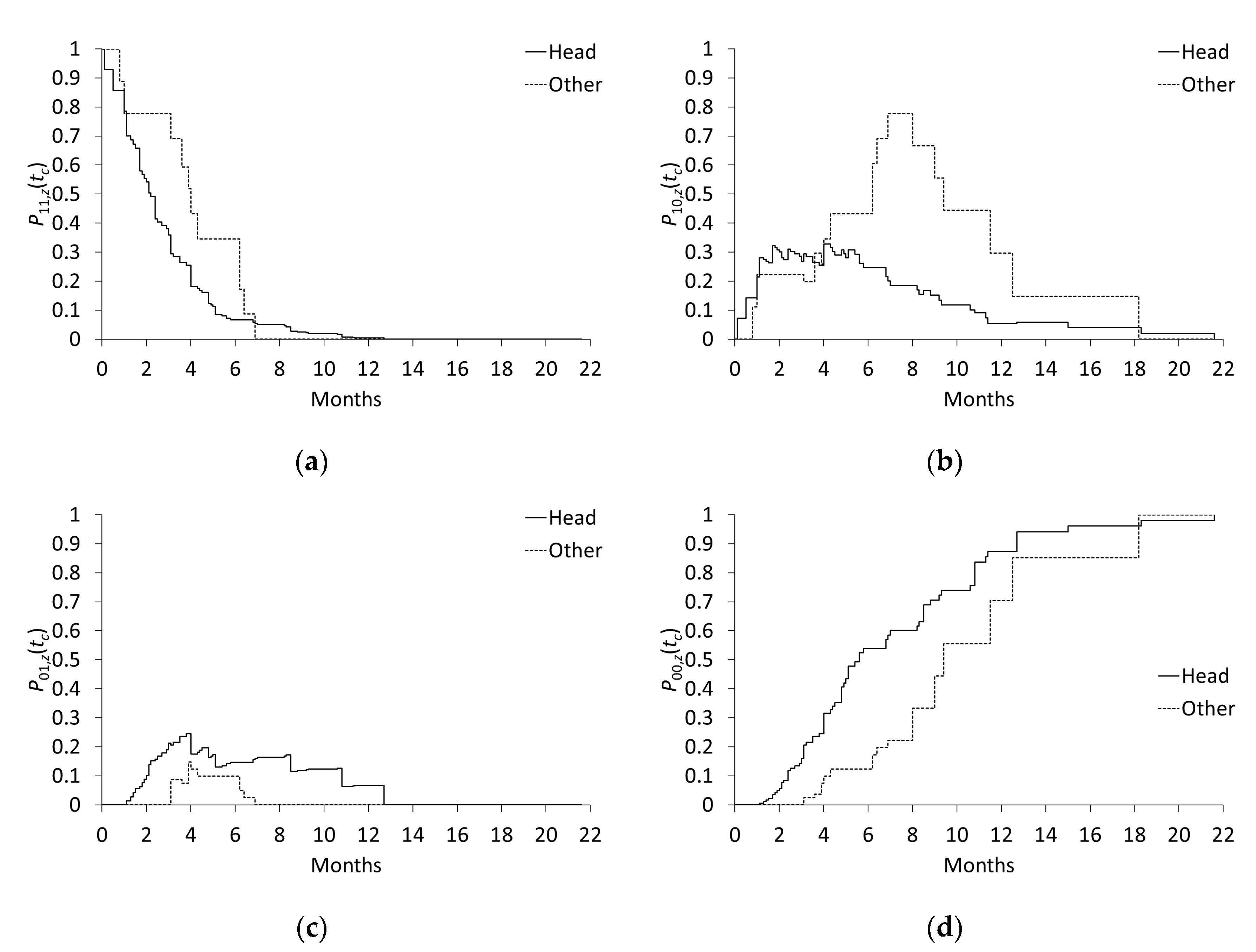
Next, we applied the approach proposed in this article. Figure 2 shows ${\widehat{P}}_{kl,z}\left(t_c\right)$ in each subgroup when the cut-off point $t_c$ was changed from 0 to 21.6 (months). The proportions of activated and inert subjects decreased and increased monotonically over time, respectively, as shown in Figure 2a,d; this is to be expected given Proposition 2. Figure 2b shows that the proportion of causative subjects is lower in the pancreatic head subgroup than in the other subgroup. Figure 2c shows that the proportion of preventive subjects was small, especially in the other subgroup. 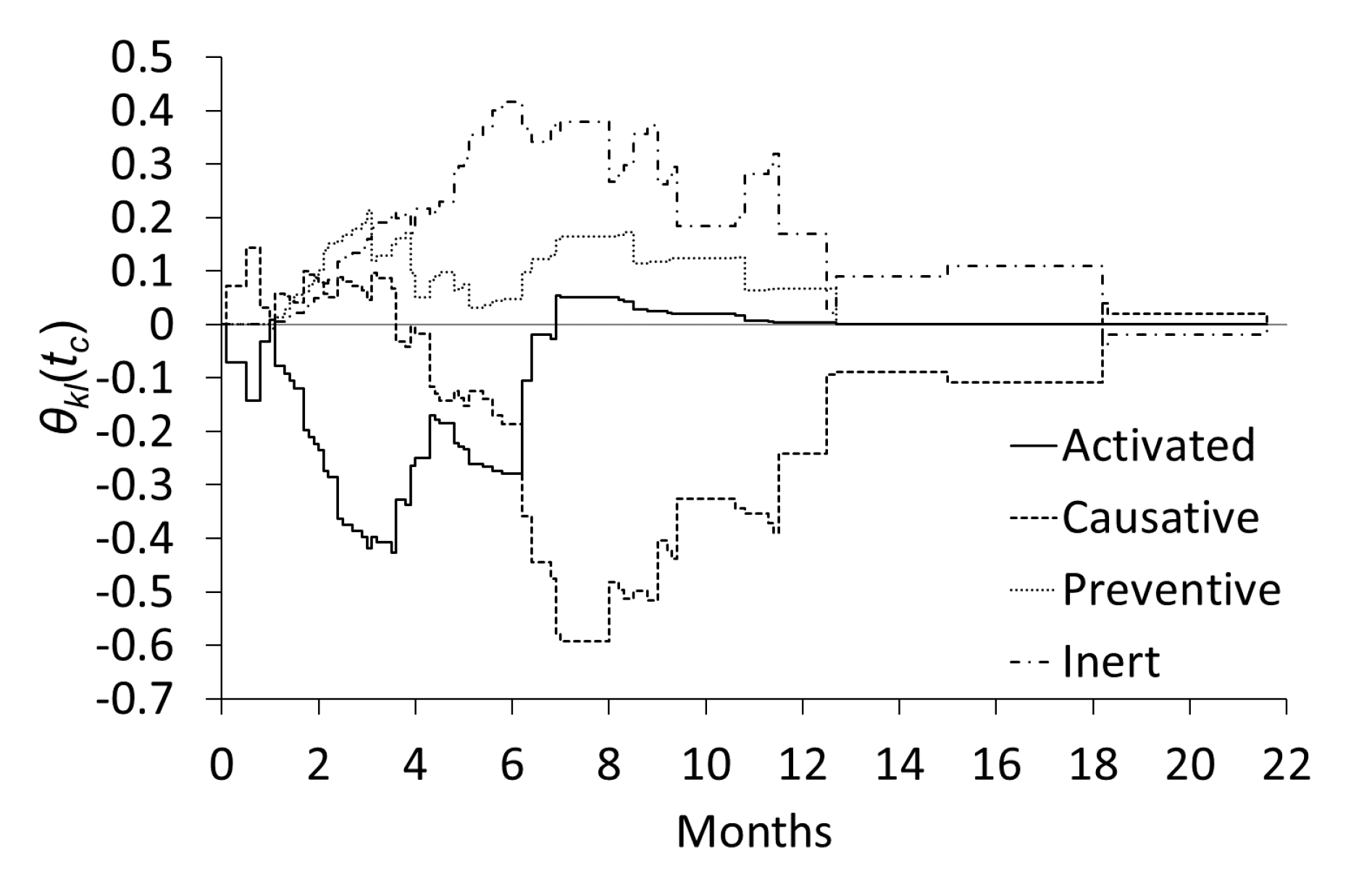Figure 3 shows the differences in the estimated proportions between the two subgroups; i.e., ${\widehat{\theta }}_{kl}\left(t_c\right)$ in (7). In Figure 3, we can clearly see that the cancer site is “depleted-activated” until approximately six months. Then, over the period from 6 to 12 months, the cancer site is “depleted-causative.”

Figure 2. Response type proportions in the pancreatic head and “other” subgroups: (a) activated (type 11) subjects; (b) causative (type 10) subjects; (c) preventive (type 01) subjects; (d) inert (type 00) subjects.

Figure 3. Differences in the proportions of type $kl$ subjects between the pancreatic head and “other” subgroups.

The estimates of ${\overline{P}}_{kl}$ in Definition 2 and ${\overline{\theta }}_{kl}$ in Proposition 1 are summarized in Table 2. In the table, ${\widehat{\overline{\theta }}}_{10}=-0.145$ implies that the mean proportion of causative subjects in the pancreatic head subgroup on the interval [0, 21.6] (12.9%) was 14.5% lower than that in the other subgroup (27.4%). This indicates that the cancer site is “depleted-causative”. However, for some subjects, the cancer site might be “activated-preventive” because ${\widehat{\overline{\theta }}}_{01}=0.057$, although the absolute value is smaller than that of ${\widehat{\overline{\theta }}}_{10}$ (−0.145). The cancer site might also be considered as “depleted-activated” because ${\widehat{\overline{\theta }}}_{11}=-0.062$. In the context of prediction and prognosis, as $\left|{\widehat{\overline{\theta }}}_{10}\right|>\left|{\widehat{\overline{\theta }}}_{01}\right|>0$, it is concluded that the cancer site would be a predictive factor of the effectiveness of radiation, and possibly also of the harm caused by radiation, albeit to a lesser extent.

Table 2. Restricted mean probabilities (RMPs) of the four response types by subgroups of cancer site and the RMP differences between the two subgroups.

Response Type	Subgroup	$\mathbf{RMP}\left({\overline{\mathit{P}}}_{\mathit{k}\mathit{l}}\right)$	$\mathbf{RMP}\mathbf{Difference}\left({\overline{\mathit{\theta }}}_{\mathit{k}\mathit{l}}\right)(95\%\mathbf{CI}{}^1)$
Activated (Type 11)	Pancreatic head	0.126	−0.062 (−0.134, 0.017)
	Other	0.188
Causative (Type 10)	Pancreatic head	0.129	−0.145 (−0.267, −0.026)
	Other	0.274
Preventive (Type 01)	Pancreatic head	0.072	0.057 (0.010, 0.119)
	Other	0.015
Inert (Type 00)	Pancreatic head	0.673	0.149 (−0.007, 0.307)
	Other	0.524

¹ Confidence intervals (CIs) were yielded as percentiles for the bootstrap distribution with 2000 samples.

The results generated using our approach were similar to those obtained via the current standard analysis; however, the magnitude was different. The difference is attributed to ${\widehat{\overline{\theta }}}_{01}=0.057\ne 0$, where our approach could not rule out, based on the data, a harmful effect of radiation in some subjects, especially in the pancreatic head subgroup. The value of ${\widehat{\delta }}^{\prime }$ estimated by the current standard analysis was −4.439, while it is converted to −0.201 ($-4.349/21.6$); this is 0.057 less than the value of ${\widehat{\overline{\theta }}}_{10}$ (−0.145) derived by our approach, as seen in Corollary 1. Similarly, ${\widehat{\gamma }}^{\prime }=-0.106$ is converted to −0.005 ($-0.106/21.6$); this is 0.057 larger than the value of ${\widehat{\overline{\theta }}}_{11}$ (−0.062). As a result, ${\widehat{\gamma }}^{\prime }$ is closer to zero than ${\widehat{\overline{\theta }}}_{11}$.

5. Conclusion

In this article, we extended the concept of the covariate effect type proposed by Chiba [3] from the case with a binary outcome to cases with time-to-event and continuous outcomes. This was achieved by using all cut-off points on the interval $\left[t_a, t_b\right]$, where the respective values of $t_a$ and $t_b$ are zero and the truncation time in a case with a time-to-event outcome and the minimum and maximum observed values in a case with a continuous outcome. A proportion of the $kl$ subjects for each cut-off point is $P_{kl}\left(t_c\right)$ in (6), and the mean of $P_{kl}\left(t_c\right)$ is the RMP, ${\overline{P}}_{kl}$, in Definition 2. As discussed in Section 2 and Section 3, the RMP is related to the arithmetic mean, which corresponds to the RMST for a case with a time-to-event outcome.

In some studies, a covariate of interest may be a continuous variable, rather than a binary variable discussed in this article. Unfortunately, our approach cannot be applied for a continuous covariate. However, a continuous covariate can be partitioned into two subgroups by finding the optimal threshold value to split it using a popular method such as receiver operating characteristic (ROC) curve analysis [19]. Recently, partitioning methods based on a combination of multivariate covariates have also been discussed [20]. These methods will facilitate the use of our approach.

Our measures of covariate effect types can easily be calculated by merging two data sets for the experimental and control arms including the rows of times and survival probabilities, which are automatically generated using commercial software such as SAS (SAS Institute, Cary, NC, USA) and R (R Foundation for Statistical Computing, Vienna, Austria). For example, to derive ${\widehat{P}}_{11}\left(t_c\right)={\widehat{S}}_1\left(t_{c-1}\right){\widehat{S}}_0\left(t_{c-1}\right)$, we can use a procedure to generate a Kaplan–Meier plot. Then, we obtain respective data sets including $\left\{t_{j_1}^1, {\widehat{S}}_1\left(t_{c-1}\right)\right\}$ and $\left\{t_{j_0}^0, {\widehat{S}}_0\left(t_{c-1}\right)\right\}$. ${\widehat{P}}_{11}\left(t_c\right)$ is derived by merging these two data sets. The RMP estimate, ${\widehat{\overline{P}}}_{11}$, is calculated by summing the areas of rectangles, which are calculated by applying a lag function. This process to estimate ${\overline{P}}_{kl}$ can be applied to a case with a continuous outcome by setting the minimum value of the outcome to zero, i.e., by using $t_j-t_1$. It is also easy to extend the method to observational studies by using a weighted survival curve [21] derived based on the propensity score [22].

A limitation of our approach is the requirement that the assumption of independent potential outcomes (Assumption 2) is used when estimating the measures of covariate effect types. Unfortunately, we cannot verify whether this assumption holds in actual studies based on the observed data. Additional work is necessary to develop a simple method to estimate our measures of covariate effect types without using the assumption of independent potential outcomes.

Current standard analysis is suitable for assessing prediction and prognosis of a covariate when ${\overline{\theta }}_{01}=0$, which implies that a covariate is not predictable for the effectiveness of the control treatment (or for the harm caused by the experimental treatment). However, when ${\overline{\theta }}_{01}\ne 0$, whether the current approach is appropriate is somewhat questionable unlike for our approach. Thus, our approach can supplement the current standard analysis, despite the limitation of requiring the assumption of independent potential outcomes.