Nonlinear Systems of Volterra Equations with Piecewise Smooth Kernels: Numerical Solution and Application for Power Systems Operation

Abstract

The evolutionary integral dynamical models of storage systems are addressed. Such models are based on systems of weakly regular nonlinear Volterra integral equations with piecewise smooth kernels. These equations can have non-unique solutions that depend on free parameters. The objective of this paper was two-fold. First, the iterative numerical method based on the modified Newton–Kantorovich iterative process is proposed for a solution of the nonlinear systems of such weakly regular Volterra equations. Second, the proposed numerical method was tested both on synthetic examples and real world problems related to the dynamic analysis of microgrids with energy storage systems.

1. Introduction

The conventional models of dynamical systems in various fields of physics, engineering, energy, economics and other fields are based on various nonstandard classes of functional equations including differential, integral and integral–differential with various delay types. Such mathematical tools are able to properly describe the process of interest and it is the only way to do it properly in most of the cases. Integral equations with delays model the various important classes of the dynamical processes. One of the most interesting classes of functional equations with delays is the evolutionary Volterra integral equations (VIE) [1,2].

The Volterra equation is of course the classical problem, which has been intensively studied during the last century. However, only a few authors have considered these equations with discontinuous kernels because of the fundamental difficulty of such equations. The integral equations of the second kind with discontinuous kernel were considered by Evans [3]. The uniform approximation theory for integral equations with discontinuous kernels was constructed by Anselone [4]. The sufficient conditions of solution existence of the linear VIE with jump discontinuity on the single curve were derived by Denisov and Lorenzi [5]. The papers [6,7,8] are devoted to a numerical treatment of integral dynamical systems described, using the nonlinear Volterra integral equations with unknown functions in the lower limits of integration. This type of equations are also connected to the optimal control problems in macro-economical Vintage Capital Management (VCM), which was discussed in a series of publications by Hritonenko and Yatsenko [9]. It is to be noted that the Volterra models take into account the memory effects of the system when the past states influence the present. Such evolutionary integral dynamic models are widely used in various applications including economics, ecology and population dynamics studies, see monograph [9], papers [10,11,12] and references therein. We refer readers to monograph [13] as an excellent introduction to the theory of VIE of the first kind with variable limits of integration.

It is to be outlined that all these models are related to the theory of VIE of the 1st kind with discontinuous kernels along the finite number of continuous curves recently introduced by Sidorov [14,15]. The existence of a continuous solution depending on free parameters and sufficient conditions for the existence of a unique continuous solution of the systems VIE of the 1st kind with discontinuous kernels were derived in [16]. The class of Volterra operator equations of the first kind with piecewise continuous kernels is studied in [17]. The problem of the generalized solution (in the Sobolev–Schwartz sense) to the Volterra equations with piecewise continuous kernels was considered in [18]. Convergence of the successive approximation method for construction of the main solutions in the sense of Kantorovich of nonlinear Volterra equations is proved in [19]. For systematic studies of VIE of the 1st kind with discontinuous kernels readers may refer to book [20] and part 1 in [21].

One of the prominent fields of applications of the VIE is the mathematical modeling of power systems [22]. The Volterra model can effectively generalize conventional discrete integral model and take into account both state of health of the storage and the availability of generation/storage of the microgrid as shown in [23]. The applicability of the linear system of VIEs to model the community of microgrids (MGs) with storage system is first demonstrated in [24].

The linear Volterra models are not able to handle the various important features of the contemporary storage systems such as the nonlinear dependence of the storage efficiency on state of charge or the complex processes of storage degradation. The objective of the present research was to report on the iterative numerical method based on the modified Newton–Kantorovich procedure applied to the system of nonlinear Volterra integral equations. The contribution of this paper is an iterative numerical method (equipped with the convergence theorem), which can use both the piecewise constant approximation and polynomial collocation method.

The efficiency of proposed methods are based both on toy examples with synthetic data and a real dataset from the dynamic models of a AC/DC hybrid isolated power system consisting of four power grids with renewable generation units and energy storage systems.

The remainder of this paper is structured as follows. In Section 1, the problem statement is formulated. Section 2 is dedicated to the modified Newton–Kantorovich iterative process’ application to the nonlinear systems of VIEs. Section 3 deals with the discretization process of the system of linear integral equation appearing on each step of proposed iterative process in Section 2. The constructed theory and numerical method are illustrated on model examples in Section 4. Storage system analysis in the microgrid, using the system of the Volterra equation, is fulfilled in Section 5. The concluding remarks finalize the paper.

2. Problem Statement

Let us consider the following nonlinear system of the Volterra integral equations of the first kind

$$\left\{\begin{array}{c}\underset{0}{\overset{t}{\int }}{h}_1(t,s,x_1\left(s\right),x_2\left(s\right),\cdots ,x_n\left(s\right))ds-f_1\left(t\right)=0,\hfill \\ \underset{0}{\overset{t}{\int }}{h}_2(t,s,x_1\left(s\right),x_2\left(s\right),\cdots ,x_n\left(s\right))ds-f_2\left(t\right)=0,\hfill \\ ⋮\hfill \\ \underset{0}{\overset{t}{\int }}{h}_n(t,s,x_1\left(s\right),x_2\left(s\right),\cdots ,x_n\left(s\right))ds-f_n\left(t\right)=0,\hfill \end{array}\right.$$

(1)

where $t\in [0,T]$ and kernels $h_i(t,s,x_1\left(s\right),x_2\left(s\right),\cdots ,x_n\left(s\right))$ are jump discontinuous on the curves ${\alpha }_j\left(t\right),$$j=1,2,\cdots ,n-1,$ and can be defined as

$$h_i(t,s,x_1\left(s\right),x_2\left(s\right),\cdots ,x_n\left(s\right))=\left\{\begin{array}{c}{K}_{i1}(t,s)G_{i1}(s,x_1\left(s\right)),(t,s)\in m_1,\hfill \\ K_{i2}(t,s)G_{i2}(s,x_2\left(s\right)),(t,s)\in m_2,\hfill \\ ⋮\hfill \\ K_{in}(t,s)G_{in}(s,x_n\left(s\right)),(t,s)\in m_n.\hfill \end{array}\right.$$

(2)

Here $m_j=\left\{(t,s)\right|{\alpha }_{j-1}\left(t\right)<s\le {\alpha }_j\left(t\right)\}$, ${\alpha }_0\left(t\right)=0$, ${\alpha }_n\left(t\right)=t$, $i=1,2,\cdots ,n$, $j=1,2,\cdots ,n$. Functions $K_{ij}(t,s)$, $f_i\left(t\right)$, ${\alpha }_j\left(t\right)$ enjoy continuous derivatives with respect to time t for $(t,s)\in {\overline{m}}_j$, $K_{in}(t,t)\ne 0$, $0<{\alpha }_1\left(t\right)<{\alpha }_2\left(t\right)<\cdots <{\alpha }_{n-1}\left(t\right)<t$. Here ${\overline{m}}_j$ is closure of the set $m_j.$ Functions ${\alpha }_1\left(t\right),\cdots ,{\alpha }_{n-1}\left(t\right)$ are nondecreasing for $t\in [0,T]$.

Let us recall the existence and uniqueness theorem for the scalar case ($i=1$ in (1)) from [25].

Theorem 1.

Let for $t\in [0,T]$ the following conditions takes place: $K_i(t,s),G_i(s,x\left(s\right))$ are continuous, $i=1,2,\cdots ,n$, ${\alpha }_i\left(t\right)$ and $f\left(t\right)$ have continuous derivatives for t, $K_n(t,t)\ne 0$, $0={\alpha }_0\left(t\right)<{\alpha }_1\left(t\right)<\cdots <{\alpha }_{n-1}\left(t\right)<{\alpha }_n\left(t\right)=t$ for $t\in (0,T]$, ${\alpha }_i\left(0\right)=0$, $f\left(0\right)=0.$ Let the functions $G_i(s,x\left(s\right))$ satisfy Lipschitz condition

$$∥G_i(s,x_1\left(s\right))-G_i(s,x_2\left(s\right))-(x_1\left(s\right)-x_2\left(s\right))∥⩽q_i∥x_1-x_2∥,\forall x_1,x_2\in {\mathbb{R}}^1,$$

$q_n+{\displaystyle \sum _{i=1}^{n-1}}{\alpha }_i^{\prime }\left(0\right)\left|K_n{(0,0)}^{-1}(K_i(0,0)-K_{i+1}(0,0))\right|(1+q_i)<1.$ Then $\exists \tau >0$ such that Equation (1) ($i=1$) has an unique local solution in ${\mathcal{C}}_{[0,\tau ]}.$ Furthermore, if $\underset{\tau \le t\le T}{min}(t-{\alpha }_{n-1}\left(t\right))=h>0$ then solution can be constructed on $[\tau ,T],$ using the step method combined with successive approximations. Thereby Equation (1) for $i=1$ has the unique global solution in ${\mathcal{C}}_{[0,T]}$.

This result is valid for complete system (1). The proof is similar with proof of Theorem 3.2 in the monograph [20].

In the present paper, we propose an iterative method for solving such nonlinear systems. Our method employs the linearization of the integral vector-operator. To solve the systems of linear equations with discontinuous kernels arising in the iterative process, we suggest two approaches: a generalization of the direct discretization algorithm proposed in [25] and the polynomial-collocation scheme. The first approach is based on a piecewise constant approximation of exact solutions and has the first order of accuracy. The second approach uses the polynomial approximation of exact solutions and allows us to derive more accurate solutions. The proposed Volterra models and numerical methods are applied to perform the dynamic analysis of microgrids with energy storage following [24].

3. Description of the Iterative Approximate Method

Let $P_i$ denotes the left hand side of i-th equation of the system (1):

$$P_i=\sum _{j=1}^n\underset{{\alpha }_{j-1}\left(t\right)}{\overset{{\alpha }_j\left(t\right)}{\int }}{K}_{ij}(t,s)G_{ij}(s,x_j\left(s\right))ds-f_i\left(t\right),$$

(3)

and X denotes the desired vector of functions, and F denotes the vector of source functions $f_i$

$$X=\left(\begin{array}{c}{x}_1\left(t\right)\\ x_2\left(t\right)\\ ⋮\\ x_n\left(t\right)\end{array}\right),F=\left(\begin{array}{c}{f}_1\left(t\right)\\ f_2\left(t\right)\\ ⋮\\ f_n\left(t\right)\end{array}\right).$$

We also introduce a matrix integral operator

$$P\left(X\right)\equiv \left(\begin{array}{cccc}{P}_{11}& P_{12}& \cdots & P_{1n}\\ P_{21}& P_{22}& \cdots & P_{2n}\\ ⋮& ⋮& \ddots & ⋮\\ P_{n1}& P_{n2}& \cdots & P_{nn}\end{array}\right)\left(\begin{array}{c}{x}_1\\ x_2\\ ⋮\\ x_n\end{array}\right)-\left(\begin{array}{c}{f}_1\\ f_2\\ ⋮\\ f_n\end{array}\right),$$

(4)

whose components are nonlinear integral operators

$$\left(P_{ij}x\right)\left(t\right)\equiv \underset{{\alpha }_{j-1}\left(t\right)}{\overset{{\alpha }_j\left(t\right)}{\int }}{K}_{ij}(t,s)G_{ij}(s,x\left(s\right))ds,i,j=1,2,\cdots ,n.$$

Let us rewrite system (1) in the operator form as follows

$$P\left(X\right)=0.$$

(5)

To construct an iterative numerical method for solving Equation (5), the following modified Newton–Kantorovich scheme [26] is employed

$$X^{m+1}=X^m-{\left[P^{\prime }\left(X^0\right)\right]}^{-1}\left(P\left(X^m\right)\right),m=0,1,2,\cdots$$

(6)

where $X^0=\left(\begin{array}{c}{x}_1^0\left(t\right)\\ x_2^0\left(t\right)\\ ⋮\\ x_n^0\left(t\right)\end{array}\right)$ is the vector in the initial approximation function, and the solution of (5) is defined as the limit $X^{*}=\underset{m\to \infty }{lim}{X}^m$. Derivative $P^{\prime }\left(X^0\right)$ of operator (4) is as follows

$$\left(\begin{array}{cccc}\frac{\partial P_{11}}{\partial x_1\left(t\right)}& \frac{\partial P_{12}}{\partial x_2\left(t\right)}& \cdots & \frac{\partial P_{1n}}{\partial x_n\left(t\right)}\\ \frac{\partial P_{21}}{\partial x_1\left(t\right)}& \frac{\partial P_{22}}{\partial x_2\left(t\right)}& \cdots & \frac{\partial P_{2n}}{\partial x_n\left(t\right)}\\ ⋮& ⋮& \ddots & ⋮\\ \frac{\partial P_{n1}}{\partial x_1\left(t\right)}& \frac{\partial P_{n2}}{\partial x_2\left(t\right)}& \cdots & \frac{\partial P_{nn}}{\partial x_n\left(t\right)}\end{array}\right)\left(\begin{array}{c}{x}_1^0\\ x_2^0\\ ⋮\\ x_n^0\end{array}\right).$$

(7)

Here the components $\left(\frac{\partial P_{ij}}{\partial x_j\left(t\right)}\right)\left(x_j^0\right),i,j=1,2,\cdots ,n,$ are defined as follows

$$\left(\frac{\partial P_{ij}}{\partial x_j\left(t\right)}\right)\left(x_j^0\right)\left(t\right)=\underset{\omega \to 0}{lim}\frac{P_{ij}(x_j^0+\omega x)-P_{ij}\left(x_j^0\right)}{\omega }=$$

$$=\underset{\omega \to 0}{lim}\frac{1}{\omega }\underset{{\alpha }_{j-1}\left(t\right)}{\overset{{\alpha }_j\left(t\right)}{\int }}{K}_{ij}(t,s)[G_{ij}(s,x_j^0\left(s\right)+\omega x\left(s\right))-G_{ij}(s,x_j^0\left(s\right))]ds.$$

The limit transition under the sign of the integral implies:

$$\left(\frac{\partial P_{ij}}{\partial x_j\left(t\right)}\right)\left(x_j^0\right)\left(t\right)=\underset{{\alpha }_{j-1}\left(t\right)}{\overset{{\alpha }_j\left(t\right)}{\int }}{K}_{ij}(t,s)G_{i{j}_x}(s,x_j^0\left(s\right))x\left(s\right)ds,$$

where

$$G_{i{j}_x}(s,x_j^0\left(s\right))=\frac{\partial G_{ij}(s,x_j\left(s\right))}{\partial x_j}{|}_{x=x_j^0}.$$

On iterations with the number m we have an operator equation with respect to the correction $\Delta X^{m+1}=X^{m+1}-X^m$, $m=0,1,2,\dots$

$$P^{\prime }\left(X^0\right)\Delta X^{m+1}=-P\left(X^m\right),$$

which in expanded form is equivalent to the following system of equations

$$\left\{\begin{array}{c}{\displaystyle \sum _{j=1}^n}\underset{{\alpha }_{j-1}\left(t\right)}{\overset{{\alpha }_j\left(t\right)}{\int }}{K}_{1j}(t,s)G_{1j}(s,x_j^0\left(s\right))\Delta x_j^{m+1}\left(s\right)ds=f_1\left(t\right)-{\displaystyle \sum _{j=1}^n}\underset{{\alpha }_{j-1}\left(t\right)}{\overset{{\alpha }_j\left(t\right)}{\int }}{K}_{1j}(t,s)G_{1j}(s,x_j^m\left(s\right))ds,\hfill \\ {\displaystyle \sum _{j=1}^n}\underset{{\alpha }_{j-1}\left(t\right)}{\overset{{\alpha }_j\left(t\right)}{\int }}{K}_{2j}(t,s)G_{2j}(s,x_j^0\left(s\right))\Delta x_j^{m+1}\left(s\right)ds=f_2\left(t\right)-{\displaystyle \sum _{j=1}^n}\underset{{\alpha }_{j-1}\left(t\right)}{\overset{{\alpha }_j\left(t\right)}{\int }}{K}_{1j}(t,s)G_{2j}(s,x_j^m\left(s\right))ds,\hfill \\ ⋮\hfill \\ {\displaystyle \sum _{j=1}^n}\underset{{\alpha }_{i-1}\left(t\right)}{\overset{{\alpha }_i\left(t\right)}{\int }}{K}_{nj}(t,s)G_{nj}(s,x_j^0\left(s\right))\Delta x_j^{m+1}\left(s\right)ds=f_n\left(t\right)-{\displaystyle \sum _{j=1}^n}\underset{{\alpha }_{j-1}\left(t\right)}{\overset{{\alpha }_j\left(t\right)}{\int }}{K}_{1j}(t,s)G_{nj}(s,x_j^m\left(s\right))ds.\hfill \end{array}\right.$$

The latter system, after a number of simplifications, is brought to mind

$$\left\{\begin{array}{c}{\displaystyle \sum _{j=1}^n}\underset{{\alpha }_{j-1}\left(t\right)}{\overset{{\alpha }_j\left(t\right)}{\int }}{K}_{1j}(t,s)G_{1j}(s,x_j^0\left(s\right))x_j^{m+1}\left(s\right)ds={\mathsf{\Psi }}_1^m\left(t\right),\hfill \\ {\displaystyle \sum _{j=1}^n}\underset{{\alpha }_{j-1}\left(t\right)}{\overset{{\alpha }_j\left(t\right)}{\int }}{K}_{2j}(t,s)G_{2j}(s,x_j^0\left(s\right))x_j^{m+1}\left(s\right)ds={\mathsf{\Psi }}_2^m\left(t\right),\hfill \\ ⋮\hfill \\ {\displaystyle \sum _{j=1}^n}\underset{{\alpha }_{i-1}\left(t\right)}{\overset{{\alpha }_i\left(t\right)}{\int }}{K}_{nj}(t,s)G_{nj}(s,x_j^0\left(s\right))x_j^{m+1}\left(s\right)ds={\mathsf{\Psi }}_n^m\left(t\right).\hfill \end{array}\right.,m=0,1,2,\cdots$$

(8)

where

$${\mathsf{\Psi }}_i^m\left(t\right)=f_i\left(t\right)-{\displaystyle \sum _{j=1}^n}\underset{{\alpha }_{j-1}\left(t\right)}{\overset{{\alpha }_j\left(t\right)}{\int }}{K}_{ij}(t,s)[G_{i{j}_x}(s,x_j^0\left(s\right))x_j^m\left(s\right)-G_{ij}(s,x_j^m\left(s\right))]ds.$$

System (8) is the system of linear Volterra integral equations with discontinuous kernels $K_{ij}(t,s)G_{ij}(s,x_j^0\left(s\right))$, $i=1,2,\cdots ,n$, $j=1,2,\cdots ,n$, which do not change from one iteration to another. A numerical method for solving similar systems of equations involved in iterative process (6) is proposed below.

The Convergence Theorem

Let ${\overline{C}}_{[0,T]}$ be a Banach vector-space of continuous vector-functions

$${\overline{C}}_{[0,T]}=\left\{X=\left(x_1\left(t\right),x_2\left(t\right),\dots ,x_n\left(t\right)\right):x_i\left(t\right)\in C_{[0,T]},i=\overline{1,n}\right\}$$

equipped with the norm

$${\parallel X\parallel }_{{\overline{C}}_{[0,T]}}=\underset{i=\overline{1,n}}{max}\parallel x_i{\parallel }_{C_{[0,T]}},\mathrm{where}\parallel x_i{\parallel }_{C_{[0,T]}}=\underset{t\in [0,T]}{max}\left|x_i\left(t\right)\right|,i=\overline{1,n}.$$

The following theorem of convergence (based on the general theory proposed in classical monograph [26], see Theorem 6, page 532) for the iterative process (6) takes place.

Theorem 2.

Let the operator P has a continuous second derivative in the sphere ${\mathsf{\Omega }}_0(\parallel X-X^0{\parallel }_{{\overline{C}}_{[0,T]}}⩽r)$ and the following conditions hold:

• Equation (8) has a unique solution for $m=0$, i.e., there exists ${\mathsf{{\rm Y}}}_0={\left[P^{\prime }\left(X^0\right)\right]}^{-1}$;
• $\parallel \Delta X^1\parallel ⩽\eta ,$ where $\Delta X^m=X^m-X^{m-1},m=0,1,\dots .$;
• $\parallel {\mathsf{{\rm Y}}}_0{P}^{″}\left(X\right)\parallel ⩽L,X\in {\mathsf{\Omega }}_0$.

If also $h=L\eta <\frac{1}{2}\mathrm{and}\frac{1-\sqrt{1-2h}}{h}\eta ⩽r⩽\frac{1+\sqrt{1-2h}}{h}\eta ,$ then Equation (5) has a unique solution $X^{*}$ in ${\mathsf{\Omega }}_0$, process (6) converges to $X^{*}$, and the velocity of convergence is estimated by the inequality

$$\parallel X^{*}-X^m\parallel ⩽\frac{\eta }{h}{(1-\sqrt{1-2h})}^{m+1},m=0,1,\dots .$$

Proof. 

In order to prove this theorem, one must show that Equation (8) is uniquely solvable (including the case $m=0$), i.e., condition 1 of the theorem holds. The solvability of linear systems of such Volterra integral equations was discussed in monograph [20], chapter 3. Condition 2 follows from condition 1. Indeed, having obtained a bounded solution of a linear system from condition, one can estimate it and obtain a constant $\eta .$

A further argumentation is performed under conditions provided the uniqueness of solution for such systems (see [20] for details).

Let us also verify the boundedness of the second derivative $\left[P^{″}\left(X^0\right)\right](X,\overline{X})$ for estimating the constant L in condition 3. The second derivative of the operator P is a bilinear integral operator having the following form

$$\left[P^{″}\left(X^0\right)\right](X,\overline{X})=\underset{\omega \to 0}{lim}\frac{\left[P^{\prime }(X^0+\omega \overline{X})\right]\left(X\right)-\left[P^{\prime }\left(X^0\right)\right]\left(X\right)}{\omega }=\underset{0}{\overset{t}{\int }}K(t,s)G_{xx}(s,X^0\left(s\right))X\left(s\right)\overline{X}\left(s\right)ds$$

with the components defined as follows

$$\left[\frac{{\partial }^2{P}_{ij}\left(x_j^0\right)}{{(\partial x_j)}^2}\right](x,\overline{x})\left(t\right)=\underset{{\alpha }_{j-1}\left(t\right)}{\overset{{\alpha }_j\left(t\right)}{\int }}{K}_{ij}(t,s)G_{i{j}_{xx}}(s,x_j^0\left(s\right))x\left(s\right)\overline{x}\left(s\right)ds,G_{i{j}_{xx}}(s,x_j^0\left(s\right))=\frac{{\partial }^2{G}_{ij}(s,x_j\left(s\right))}{{(\partial x_j)}^2}{|}_{x=x_j^0}.$$

Therefore, assuming additionally that the functions $G_{ij}(s,x\left(s\right))$ have bounded second derivatives with respect to x in the neighborhood of initial approximation $X^0$, we can conclude that the operator $\left[P^{″}\left(X^0\right)\right](X,\overline{X})$ is bounded.  □

4. Discretization of the System of Linear Integral Equations

4.1. Problem Formulation

In this paragraph, we propose a numerical method for solving systems of linear integral equations arising at each step of the iterative process (6).

Let us consider the following system of linear integral equations of the first kind

$$\left\{\begin{array}{c}{\displaystyle \sum _{j=1}^n}\underset{{\alpha }_{j-1}\left(t\right)}{\overset{{\alpha }_j\left(t\right)}{\int }}{h}_1(t,s)x_j\left(s\right)ds=f_1\left(t\right),\hfill \\ {\displaystyle \sum _{j=1}^n}\underset{{\alpha }_{j-1}\left(t\right)}{\overset{{\alpha }_j\left(t\right)}{\int }}{h}_2(t,s)x_j\left(s\right)ds=f_2\left(t\right),\hfill \\ ⋮\hfill \\ {\displaystyle \sum _{j=1}^n}\underset{{\alpha }_{j-1}\left(t\right)}{\overset{{\alpha }_j\left(t\right)}{\int }}{h}_n(t,s)x_j\left(s\right)ds=f_n\left(t\right).\hfill \end{array}\right.,$$

(9)

functions $h_i(t,s),i=1,2,\cdots ,n,$ undergo a finite discontinuity on the curves ${\alpha }_j\left(t\right),j=1,2,\cdots ,n-1$ and

$$h_i(t,s)=\left\{\begin{array}{cc}{K}_{i1}:=K_{i1}(t,s)G_{i1}(s,x_j^0\left(s\right)),\hfill & \mathrm{if}{\alpha }_0\left(t\right)<s\le {\alpha }_1\left(t\right);\hfill \\ K_{i2}:=K_{i2}(t,s)G_{i2}(s,x_j^0\left(s\right)),\hfill & \mathrm{if}{\alpha }_1\left(t\right)<s\le {\alpha }_2\left(t\right);\hfill \\ ⋮\hfill \\ K_{in}:=K_{in}(t,s)G_{in}(s,x_j^0\left(s\right)),\hfill & \mathrm{if}{\alpha }_{n-1}\left(t\right)<s\le {\alpha }_n\left(t\right).\hfill \end{array}\right.$$

Here ${\alpha }_0\left(t\right)\equiv 0,{\alpha }_0\left(t\right)<{\alpha }_1\left(t\right)<\cdots <{\alpha }_n\left(t\right)\equiv t,f\left(0\right)=0$. The new kernels $K_{ij}(t,s)$ and right-hand side $f_i\left(t\right)$ are continuous and sufficiently smooth functions introduced to simplify the exposition. The functions ${\alpha }_j\left(t\right)\in C^1[0,T]$ are nondecreasing. Also ${\alpha }_1^{\prime }\left(0\right)\le {\alpha }_2^{\prime }\left(0\right)\le \cdots \le {\alpha }_{n-1}^{\prime }\left(0\right)<1$.

4.2. Piecewise Constant Approximation

In order to construct a numerical solution of (9) on the segment $[0,T]$ (under the conditions of existence of a single continuous solution), we introduce a grid of nodes (not necessarily uniform)

$$0=t_0<t_1<t_2<\cdots <t_N=t,h=\underset{j=1,2,\cdots ,N}{max}(t_j-t_{j-1})=\mathcal{O}\left(N^{-1}\right).$$

An approximate solution of the system (9) will be sought in the form of a vector of piecewise constant functions

$$X^N\left(t\right)=\left(\begin{array}{c}{\displaystyle \sum _{j=1}^N}{x}_1^j{\delta }_j\left(t\right)\\ {\displaystyle \sum _{j=1}^N}{x}_2^j{\delta }_j\left(t\right)\\ ⋮\\ {\displaystyle \sum _{j=1}^N}{x}_n^j{\delta }_j\left(t\right)\end{array}\right),t\in (0,T],{\delta }_j\left(t\right)=\left\{\begin{array}{cc}1,\hfill & \mathrm{when}t\in {\Delta }_j=(t_{j-1},t_j]\hfill \\ 0,\hfill & \mathrm{when}t\notin {\Delta }_j\hfill \end{array}\right.,$$

with uncertain coefficients so far $x_i^j,i=1,2,\cdots ,n,j=1,2,\cdots ,N.$ To determine the values $x_i^0=x_i\left(0\right),i=1,2,\cdots ,n,$ we differentiate both parts of each Equation (9) by t

$$f_i\left(t\right)=\sum _{j=1}^n(\underset{{\alpha }_{j-1}\left(t\right)}{\overset{{\alpha }_j\left(t\right)}{\int }}\frac{\partial K_{ij}(t,s)}{\partial t}{x}_j\left(s\right)ds+{\alpha }_j^{\prime }\left(t\right)K_{ij}(t,{\alpha }_j\left(t\right))x_j\left({\alpha }_j\left(t\right)\right)-$$

$$-{\alpha }_{j-1}^{\prime }\left(t\right)K_{ij}(t,{\alpha }_{j-1}\left(t\right))x_j\left({\alpha }_{i-1}\left(t\right)\right)).$$

Using the latter ratio, we come to the necessity of solving a system of equations

$$\left\{\begin{array}{c}{\displaystyle \sum _{j=1}^n}{K}_{1j}(0,0)[{\alpha }_j^{\prime }\left(0\right)-{\alpha }_{j-1}^{\prime }\left(0\right)]x_j^0=f_1^{\prime }\left(0\right),\hfill \\ {\displaystyle \sum _{j=1}^n}{K}_{2j}(0,0)[{\alpha }_j^{\prime }\left(0\right)-{\alpha }_{j-1}^{\prime }\left(0\right)]x_j^0=f_2^{\prime }\left(0\right),\hfill \\ ⋮\hfill \\ {\displaystyle \sum _{j=1}^n}{K}_{nj}(0,0)[{\alpha }_j^{\prime }\left(0\right)-{\alpha }_{j-1}^{\prime }\left(0\right)]x_j^0=f_n^{\prime }\left(0\right).\hfill \end{array}\right.$$

(10)

with respect to values $x_j^0,j=1,2,\cdots ,n$. Here it is assumed that the components of the Equation (9) are such that the system of linear algebraic Equation (10) has a unique nontrivial solution.

Next, we introduce the designation $f_i^k=f_i\left(t_k\right),I=1,\dots ,n,k=1,\dots ,N$. To determine the coefficients $x_j^1$, write down each equation of the system (9) at $t=t_1$.

$$\sum _{j=1}^n\underset{{\alpha }_{j-1}\left(t_1\right)}{\overset{{\alpha }_j\left(t_1\right)}{\int }}{K}_{ij}(t_1,s)x_j\left(s\right)ds=f_i^1.$$

(11)

Since at this step, the lengths of all integration segments ${\alpha }_j\left(t_1\right)-{\alpha }_{j-1}\left(t_1\right)$ in (17) do not exceed the maximum grid step h, and the components of the approximate solution take the values $x_j^1$, $j=1,2,\cdots ,n$, then applying the quadrature formula of the midpoint rectangles, we have a system of

$$\left\{\begin{array}{c}{\displaystyle \sum _{j=1}^n}({\alpha }_j\left(t_1\right)-{\alpha }_{j-1}\left(t_1\right))K_{1j}(t_1,\frac{{\alpha }_j\left(t_1\right)+{\alpha }_{j-1}\left(t_1\right)}{2})x_j^1=f_1^1,\hfill \\ {\displaystyle \sum _{j=1}^n}({\alpha }_j\left(t_1\right)-{\alpha }_{j-1}\left(t_1\right))K_{2j}(t_1,\frac{{\alpha }_j\left(t_1\right)+{\alpha }_{j-1}\left(t_1\right)}{2})x_j^1=f_2^1,\hfill \\ ⋮\hfill \\ {\displaystyle \sum _{j=1}^n}({\alpha }_j\left(t_1\right)-{\alpha }_{j-1}\left(t_1\right))K_{nj}(t_1,\frac{{\alpha }_j\left(t_1\right)+{\alpha }_{j-1}\left(t_1\right)}{2})x_j^1=f_n^1.\hfill \end{array}\right.,$$

of which shall be determined by the value of $x_j^1,j=1,2,\cdots ,n$.

Let $l_j^K$ further denote the number of the grid’s segment, which gets the value ${\alpha }_j\left(t_k\right)$, that is, the condition $t_{l_j^k-1}\le {\alpha }_j\left(t_k\right)\le t_{l_j^k}$ is satisfied.

Assume now that the values $x_j^2,x_j^3,\cdots ,x_j^{l_j^K-1},K=1,2,\cdots ,n$ are already found.

Let us transform system (9) and require the following equalities satisfaction at the point $t=t_k$

$$\left\{\begin{array}{c}{\displaystyle \sum _{j=1}^n}\underset{t_{l_j^k-1}}{\overset{{\alpha }_j\left(t_k\right)}{\int }}{K}_{1j}(t_k,s)x_j\left(s\right)ds=f_1^k-{\displaystyle \sum _{j=1}^n}\underset{{\alpha }_{j-1}\left(t_k\right)}{\overset{t_{l_j^k-1}}{\int }}{K}_{1j}(t_k,s)x_j^N\left(s\right)ds,\hfill \\ {\displaystyle \sum _{j=1}^n}\underset{t_{l_j^k-1}}{\overset{{\alpha }_j\left(t_k\right)}{\int }}{K}_{2j}(t_k,s)x_j\left(s\right)ds=f_2^k-{\displaystyle \sum _{j=1}^n}\underset{{\alpha }_{j-1}\left(t_k\right)}{\overset{t_{l_j^k-1}}{\int }}{K}_{2j}(t_k,s)x_j^N\left(s\right)ds,\hfill \\ ⋮\hfill \\ {\displaystyle \sum _{j=1}^n}\underset{t_{l_j^k-1}}{\overset{{\alpha }_j\left(t_k\right)}{\int }}{K}_{nj}(t_k,s)x_j\left(s\right)ds=f_n^k-{\displaystyle \sum _{j=1}^n}\underset{{\alpha }_{j-1}\left(t_k\right)}{\overset{t_{l_j^k-1}}{\int }}{K}_{nj}(t_k,s)x_j^N\left(s\right)ds.\hfill \end{array}\right.$$

The given approximation leads to the following system

$$\left\{\begin{array}{c}{\displaystyle \sum _{j=1}^n}{x}_j^{l_j^k}\underset{t_{l_j^k-1}}{\overset{{\alpha }_j\left(t_k\right)}{\int }}{K}_{1j}(t_k,s)ds=f_1^k-{\displaystyle \sum _{j=1}^n}\underset{{\alpha }_{j-1}\left(t_k\right)}{\overset{t_{l_j^k-1}}{\int }}{K}_{1j}(t_k,s)x_j^N\left(s\right)ds,\hfill \\ {\displaystyle \sum _{j=1}^n}{x}_j^{l_j^k}\underset{t_{l_j^k-1}}{\overset{{\alpha }_j\left(t_k\right)}{\int }}{K}_{2j}(t_k,s)ds=f_2^k-{\displaystyle \sum _{j=1}^n}\underset{{\alpha }_{j-1}\left(t_k\right)}{\overset{t_{l_j^k-1}}{\int }}{K}_{2j}(t_k,s)x_j^N\left(s\right)ds,\hfill \\ ⋮\hfill \\ {\displaystyle \sum _{j=1}^n}{x}_j^{l_j^k}\underset{t_{l_j^k-1}}{\overset{{\alpha }_j\left(t_k\right)}{\int }}{K}_{nj}(t_k,s)ds=f_n^k-{\displaystyle \sum _{j=1}^n}\underset{{\alpha }_{j-1}\left(t_k\right)}{\overset{t_{l_j^k-1}}{\int }}{K}_{nj}(t_k,s)x_j^N\left(s\right)ds.\hfill \end{array}\right.$$

(12)

For the integrals calculation in (12), the compound midpoint rectangle quadrature constructed on the auxiliary grid of nodes bound at each concrete value N to the discontinuity curve ${\alpha }_i\left(t\right)$ of kernel $K(t,s)$ is used.

It is not difficult to see that such an approximation method has the first order of accuracy and the following error estimate takes place

$${\epsilon }_N={∥X-X_N∥}_{C[0,T]}=\mathcal{O}\left(\frac{1}{N}\right).$$

Remark 1.

It should be noted that the proposed numerical approach also allows for a more accurate approximation of the solution. In particular, when using piecewise linear approximation, the order of accuracy increases by one. However, such discretized systems may have non-unique solutions (due to the discontinuities ${\alpha }_i\left(t\right),i=1,2,\cdots ,n,$ they can be under-determined or have many solutions). Taking into account this fact we suggest a new alternative numerical method below.

4.3. Polynomial Collocation Method

4.3.1. Description of the Problem

In this section, we deal with the numerical solution of the following system of VIE

$$\underset{0}{\overset{t}{\int }}H(t,s)X\left(s\right)ds=F\left(t\right),$$

(13)

where

$$H(t,s)=\left(\begin{array}{c}{h}_1(t,s)\\ h_2(t,s)\\ ⋮\\ h_n(t,s)\end{array}\right),F\left(t\right)=\left(\begin{array}{c}{f}_1\left(t\right)\\ f_2\left(t\right)\\ ⋮\\ f_n\left(t\right)\end{array}\right).$$

Here, kernels $h_i(t,s),i=1,2,\cdots ,n,$ have just discontinuities on the lines ${\alpha }_j\left(t\right),j=1,2,\cdots ,n-1$ and kernels are defined as follows

$$h_i(t,s)=\left\{\begin{array}{cc}{K}_{i1}(t,s),\hfill & \mathrm{if}{\alpha }_0\left(t\right)<s\le {\alpha }_1\left(t\right);\hfill \\ K_{i2}(t,s),\hfill & \mathrm{if}{\alpha }_1\left(t\right)<s\le {\alpha }_2\left(t\right);\hfill \\ ⋮\hfill \\ K_{in}(t,s),\hfill & \mathrm{if}{\alpha }_{n-1}\left(t\right)<s\le {\alpha }_n\left(t\right).\hfill \end{array}\right.$$

Components $x_i\left(t\right),i=1,2,\cdots ,n,$ of desired vector function $X\left(t\right)$ are defined in the domains $({\alpha }_{i-1}\left(t\right),{\alpha }_i\left(t\right)]$, i.e.,

$$X\left(t\right)=x_i\left(t\right)\mathrm{for}t\in {\alpha }_{i-1}\left(t\right)<s\le {\alpha }_i\left(t\right).$$

Here ${\alpha }_0\left(t\right)\equiv 0,{\alpha }_0\left(t\right)<{\alpha }_1\left(t\right)<\cdots <{\alpha }_n\left(t\right)\equiv t,$ for $t\in (0,T)$, ${\alpha }_i\left(0\right)=f_i\left(0\right)=0,i=1,2,\cdots ,n$. It is assumed that functions $K_{ij}(t,s)$ and $f_i\left(t\right),i,j=1,2,\cdots ,n,$ are continuous and smooth sufficiently. Functions ${\alpha }_j\left(t\right)\in C^1[0,T]$ and nondecreasing, ${\alpha }_1^{\prime }\left(0\right)\le {\alpha }_2^{\prime }\left(0\right)\le \cdots \le {\alpha }_{n-1}^{\prime }\left(0\right)<1$.

Let us rewrite the formal notation (13) as follows

$$\left\{\begin{array}{c}{\displaystyle \sum _{j=1}^n}\underset{{\alpha }_{j-1}\left(t\right)}{\overset{{\alpha }_j\left(t\right)}{\int }}{K}_{1j}(t,s)x_j\left(s\right)ds=f_1\left(t\right),\hfill \\ {\displaystyle \sum _{j=1}^n}\underset{{\alpha }_{j-1}\left(t\right)}{\overset{{\alpha }_j\left(t\right)}{\int }}{K}_{2j}(t,s)x_j\left(s\right)ds=f_2\left(t\right),\hfill \\ ⋮\hfill \\ {\displaystyle \sum _{j=1}^n}\underset{{\alpha }_{j-1}\left(t\right)}{\overset{{\alpha }_j\left(t\right)}{\int }}{K}_{nj}(t,s)x_j\left(s\right)ds=f_n\left(t\right).\hfill \end{array}\right..$$

(14)

4.3.2. Collocation

For construction of numerical solution of system (14) on $[0,T]$ (in conditions of unique continuous solution existence) let us introduce the mesh (not necessarily uniform in general)

$$0=t_0<t_1<t_2<\cdots <t_m=T,h=\underset{j=1,2,\cdots ,m}{max}(t_j-t_{j-1})=\mathcal{O}\left(m^{-1}\right).$$

As an approximate solution of the system (14), we search in the following form

$$X^m\left(t\right)=\left(\begin{array}{c}{\displaystyle \sum _{j=0}^m}{A}_{1j}{t}^j\\ {\displaystyle \sum _{j=0}^m}{A}_{2j}{t}^j\\ ⋮\\ {\displaystyle \sum _{j=0}^m}{A}_{nj}{t}^j\end{array}\right),t\in (0,T],$$

(15)

with unknown coefficients $A_{ij},i=1,2,\cdots ,n,j=0,2,\cdots ,m.$

To define the coefficients $A_{i0}=x_i\left(0\right),i=1,2,\cdots ,n,$ we differentiate Equation (14) with respect to t

$$f_i^{\prime }\left(t\right)={\displaystyle \sum _{j=1}^n}(\underset{{\alpha }_{j-1}\left(t\right)}{\overset{{\alpha }_j\left(t\right)}{\int }}\frac{\partial K_{ij}(t,s)}{\partial t}{x}_j\left(s\right)ds+{\alpha }_j^{\prime }\left(t\right)K_{ij}(t,{\alpha }_j\left(t\right))x_j\left({\alpha }_j\left(t\right)\right)-$$

$$-{\alpha }_{j-1}^{\prime }\left(t\right)K_{ij}(t,{\alpha }_{j-1}\left(t\right))x_j\left({\alpha }_{i-1}\left(t\right)\right)).$$

Using the latter equation we obtain the following system

$$\left\{\begin{array}{c}{\displaystyle \sum _{j=1}^n}{K}_{1j}(0,0)[{\alpha }_j^{\prime }\left(0\right)-{\alpha }_{j-1}^{\prime }\left(0\right)]A_{j0}=f_1^{\prime }\left(0\right),\hfill \\ {\displaystyle \sum _{j=1}^n}{K}_{2j}(0,0)[{\alpha }_j^{\prime }\left(0\right)-{\alpha }_{j-1}^{\prime }\left(0\right)]A_{j0}=f_2^{\prime }\left(0\right),\hfill \\ ⋮\hfill \\ {\displaystyle \sum _{j=1}^n}{K}_{nj}(0,0)[{\alpha }_j^{\prime }\left(0\right)-{\alpha }_{j-1}^{\prime }\left(0\right)]A_{j0}=f_n^{\prime }\left(0\right).\hfill \end{array}\right.$$

(16)

with respect to $A_{j0},j=1,2,\cdots ,n$. Here we assume that components of Equation (14) such as system of linear algebraic Equation (16) enjoys unique nontrivial solution.

To define the coefficients $A_{ij}$ each equation of the system (14) we write in the point $t=t_k$.

$$\sum _{j=1}^n\underset{{\alpha }_{j-1}\left(t_k\right)}{\overset{{\alpha }_j\left(t_k\right)}{\int }}{K}_{ij}(t_k,s)x_j\left(s\right)ds=f_i\left(t_k\right).$$

(17)

Let us require the conversion of Equation (17) (considering (15)), into the following identity:

$$\sum _{j=1}^n\underset{{\alpha }_{j-1}\left(t_k\right)}{\overset{{\alpha }_j\left(t_k\right)}{\int }}{K}_{ij}(t_k,s)\left(\sum _{l=0}^m{A}_{jl}{s}^l\right)ds=f_i\left(t_k\right).$$

(18)

The coefficients $A_{j0},j=1,2,\cdots ,n$ are already known on this stage and we can write

$$\sum _{j=1}^n\sum _{l=1}^m{A}_{jl}\underset{{\alpha }_{j-1}\left(t_k\right)}{\overset{{\alpha }_j\left(t_k\right)}{\int }}{K}_{ij}(t_k,s)s^{l}ds=f_i\left(t_k\right)-\sum _{j=1}^n{A}_{j0}\underset{{\alpha }_{j-1}\left(t_k\right)}{\overset{{\alpha }_j\left(t_k\right)}{\int }}{K}_{ij}(t_k,s)ds.$$

(19)

Let us introduce the following notations

$$F_{ik}:=f_i\left(t_k\right)-\sum _{j=1}^n{A}_{j0}\underset{{\alpha }_{j-1}\left(t_k\right)}{\overset{{\alpha }_j\left(t_k\right)}{\int }}{K}_{ij}(t_k,s)ds;i=1,2,\cdots ,n,k=1,2,\cdots ,m,$$

(20)

$$C_{ikjl}:=\underset{{\alpha }_{j-1}\left(t_k\right)}{\overset{{\alpha }_j\left(t_k\right)}{\int }}{K}_{ij}(t_k,s)s^{l}ds;i=1,2,\cdots ,n,k=1,2,\cdots ,m,j=1,2,\cdots ,n,l=1,2,\cdots ,m;$$

(21)

$$C:=\left(\begin{array}{ccccccccccccc}{C}_{1111}& C_{1112}& \dots & C_{111m}& C_{1121}& C_{1122}& \dots & C_{112m}& \dots & C_{11n1}& C_{11n2}& \dots & C_{11nm}\\ C_{1211}& C_{1212}& \dots & C_{121m}& C_{1121}& C_{1222}& \dots & C_{122m}& \dots & C_{12n1}& C_{12n2}& \dots & C_{12nm}\\ \dots & \dots & \dots & \dots & \dots & \dots & \dots & \dots & \dots & \dots & \dots & \dots & \dots \\ C_{1m11}& C_{1m12}& \dots & C_{1m1m}& C_{1m21}& C_{1m22}& \dots & C_{1m2m}& \dots & C_{1mn1}& C_{1mn2}& \dots & C_{1mnm}\\ C_{2111}& C_{2112}& \dots & C_{211m}& C_{2121}& C_{2122}& \dots & C_{212m}& \dots & C_{21n1}& C_{21n2}& \dots & C_{21nm}\\ C_{2211}& C_{2212}& \dots & C_{221m}& C_{2121}& C_{2222}& \dots & C_{222m}& \dots & C_{22n1}& C_{22n2}& \dots & C_{22nm}\\ \dots & \dots & \dots & \dots & \dots & \dots & \dots & \dots & \dots & \dots & \dots & \dots & \dots \\ C_{2m11}& C_{2m12}& \dots & C_{2m1m}& C_{2m21}& C_{2m22}& \dots & C_{2m2m}& \dots & C_{2mn1}& C_{2mn2}& \dots & C_{2mnm}\\ \dots & \dots & \dots & \dots & \dots & \dots & \dots & \dots & \dots & \dots & \dots & \dots & \dots \\ \dots & \dots & \dots & \dots & \dots & \dots & \dots & \dots & \dots & \dots & \dots & \dots & \dots \\ \dots & \dots & \dots & \dots & \dots & \dots & \dots & \dots & \dots & \dots & \dots & \dots & \dots \\ \dots & \dots & \dots & \dots & \dots & \dots & \dots & \dots & \dots & \dots & \dots & \dots & \dots \\ C_{n111}& C_{n112}& \dots & C_{n11m}& C_{n121}& C_{n122}& \dots & C_{n12m}& \dots & C_{n1n1}& C_{n1n2}& \dots & C_{n1nm}\\ C_{n211}& C_{n212}& \dots & C_{n21m}& C_{n121}& C_{n222}& \dots & C_{n22m}& \dots & C_{n2n1}& C_{n2n2}& \dots & C_{n2nm}\\ \dots & \dots & \dots & \dots & \dots & \dots & \dots & \dots & \dots & \dots & \dots & \dots & \dots \\ C_{nm11}& C_{nm12}& \dots & C_{nm1m}& C_{nm21}& C_{nm22}& \dots & C_{nm2m}& \dots & C_{nmn1}& C_{nmn2}& \dots & C_{nmnm}\end{array}\right)$$

(22)

$$A:=\left(\begin{array}{c}{A}_{11}\\ A_{12}\\ \dots \\ A_{1m}\\ A_{21}\\ A_{22}\\ \dots \\ A_{2m}\\ \dots \\ A_{n1}\\ A_{n2}\\ \dots \\ A_{nm}\end{array}\right),F:=\left(\begin{array}{c}{F}_{11}\\ F_{12}\\ \dots \\ F_{1m}\\ F_{21}\\ F_{22}\\ \dots \\ F_{2m}\\ \dots \\ F_{n1}\\ F_{n2}\\ \dots \\ F_{nm}\end{array}\right).$$

(23)

As a result, in order to define the coefficients $A_{ij}$ one must solve the following SLAE of dimension $(n·m)\times (n·m)$

$$C·A=F.$$

(24)

Elements of the matrices (22) and (23) can be represented as follows

$$C_{\left[\right(i-1)·m+k]\left[\right(j-1)·m+l]}=C_{ikjl};$$

(25)

$$A_{\left[\right(j-1)·m+l]}=A_{jl};$$

(26)

$$F_{\left[\right(i-1)·m+k]}=F_{ik};$$

(27)

where $i=1,2,\cdots ,n,k=1,2,\cdots ,m,j=1,2,\cdots ,n,l=1,2,\cdots ,m$.

Here, for integrals calculation in (20), (21) one must employ the compound midpoint quadrature rule constructed on the auxiliary mesh linked to the lines ${\alpha }_i\left(t\right)$ of the kernels $h_i(t,s),i=1,2,\cdots ,n$ discontinuities.

Finally, as solution to the system (24), the coefficients $A_{ij}$ are be determined and the polynomial approximation of the components of the approximate solution $X^m\left(t\right)$ is derived.

5. Numerical Results

5.1. System of Linear Integral Equations

In order to illustrate the convergence of proposed algorithm in Section 4.3.2, we consider two system of equations.

Example 1.

($n=2$).

$$\left\{\begin{array}{c}\underset{0}{\overset{\frac{t}{2}}{\int }}(1+t+s)x_1\left(s\right)ds+\underset{\frac{t}{2}}{\overset{t}{\int }}{x}_2\left(s\right)ds=f_1\left(t\right)\hfill \\ \underset{0}{\overset{\frac{t}{2}}{\int }}(1+t-s)x_1\left(s\right)ds-\underset{\frac{t}{2}}{\overset{t}{\int }}{x}_2\left(s\right)ds=f_2\left(t\right)\hfill \end{array}\right.,t\in [0,2],$$

(28)

where

$$f_1\left(t\right)=1+sin\left(\frac{t}{2}\right)+\frac{3t}{2}·sin\left(\frac{t}{2}\right)+2cos\left(\frac{t}{2}\right)-cos\left(t\right),$$

$$f_2\left(t\right)=1+sin\left(\frac{t}{2}\right)+\frac{t}{2}sin\left(\frac{t}{2}\right)-2cos\left(\frac{t}{2}\right)+cos\left(t\right).$$

The exact solution of the system (28) is $x_1\left(t\right)=cos\left(t\right),x_2\left(t\right)=sin\left(t\right)$. The numerical solution of the system (28) is given in

Table 1. Results for the problem (28).

m	${\mathit{\epsilon }}_1$	${\mathit{t}}_{\mathbf{max}}^1$	${\mathit{\epsilon }}_2$	${\mathit{t}}_{\mathit{max}}^2$	$\mathit{\epsilon }$
2	$9.82294\times {10}^{-3}$	1.0	$6.72940\times {10}^{-2}$	2.0	$6.80072\times {10}^{-2}$
3	$1.60472\times {10}^{-3}$	1.0	$2.35676\times {10}^{-2}$	2.0	$2.36222\times {10}^{-2}$
5	$6.67315\times {10}^{-6}$	1.0	$3.95344\times {10}^{-4}$	2.0	$3.95400\times {10}^{-4}$
8	$1.72968\times {10}^{-8}$	1.0	$1.80165\times {10}^{-7}$	2.0	$1.80994\times {10}^{-7}$
12	$1.31014\times {10}^{-8}$	1.0	$4.12674\times {10}^{-9}$	2.0	$1.37360\times {10}^{-8}$
15	$2.79384\times {10}^{-8}$	1.0	$1.75046\times {10}^{-8}$	2.0	$3.29692\times {10}^{-8}$

, where m is order of approximating polynomial, ${\epsilon }_i=\underset{t\in [0,a_i\left(T\right)]}{max}|x_i^{*}\left(t\right)-x_i\left(t\right)|$, $t_{max}^i$ is the greatest error point ${\epsilon }_i,i=1,\dots ,n$, $\epsilon =\sqrt{{\displaystyle \sum _{i=1}^n}{\epsilon }_i^2}$.

Example 2.

($n=3$).

Let us consider the following system of equations

$$\left\{\begin{array}{c}\underset{0}{\overset{\frac{t}{3}}{\int }}(1+t+s)x_1\left(s\right)ds+\underset{\frac{t}{3}}{\overset{\frac{2t}{3}}{\int }}{x}_2\left(s\right)ds+\underset{\frac{2t}{3}}{\overset{t}{\int }}(1+s)x_3\left(s\right)ds=f_1\left(t\right)\hfill \\ \underset{0}{\overset{\frac{t}{3}}{\int }}(1+t-s)x_1\left(s\right)ds-\underset{\frac{t}{3}}{\overset{\frac{2t}{3}}{\int }}{x}_2\left(s\right)ds+\underset{\frac{2t}{3}}{\overset{t}{\int }}(1-t)x_3\left(s\right)ds=f_2\left(t\right)\hfill \\ \underset{0}{\overset{\frac{t}{3}}{\int }}(1+\frac{t}{5}+s)x_1\left(s\right)ds+\underset{\frac{t}{3}}{\overset{\frac{2t}{3}}{\int }}(1+t-s)x_2\left(s\right)ds-\underset{\frac{2t}{3}}{\overset{t}{\int }}(1+s)x_3\left(s\right)ds=f_3\left(t\right)\hfill \end{array}\right.t\in [0,2].$$

(29)

where $f_i\left(t\right),i=1,2,3,$ are selected, the exact solution is as follows

$$x_1\left(t\right)=cos\left(t\right),x_2\left(t\right)=sin\left(t\right),x_3=\frac{1}{4}sin\left(t\right).$$

In

Table 2. Results for problem (29).

m	${\mathit{\epsilon }}_1$	${\mathit{t}}_{\mathit{max}}^1$	${\mathit{\epsilon }}_2$	${\mathit{t}}_{\mathit{max}}^2$	${\mathit{\epsilon }}_3$	${\mathit{t}}_{\mathit{max}}^3$	$\mathit{\epsilon }$
2	$1.75798\times {10}^{-3}$	0.6(6)	$3.30114\times {10}^{-3}$	1.3(3)	$6.72940\times {10}^{-2}$	2.0	$3.44752\times {10}^{-2}$
3	$2.75534\times {10}^{-4}$	0.6(6)	$3.77383\times {10}^{-3}$	1.3(3)	$4.51700\times {10}^{-3}$	2.0	$5.89245\times {10}^{-3}$
5	$1.68420\times {10}^{-6}$	0.6(6)	$2.89243\times {10}^{-5}$	1.3(3)	$9.1497\times {10}^{-5}$	2.0	$9.59747\times {10}^{-5}$
8	$7.86707\times {10}^{-10}$	0.6(6)	$6.86599\times {10}^{-9}$	1.3(3)	$4.15579\times {10}^{-8}$	2.0	$4.21286\times {10}^{-8}$
12	$1.33907\times {10}^{-9}$	0.6(6)	$1.55675\times {10}^{-9}$	1.3(3)	$1.97100\times {10}^{-10}$	2.0	$2.06287\times {10}^{-9}$
15	$1.69313\times {10}^{-9}$	0.6(6)	$1.00072\times {10}^{-9}$	1.3(3)	$1.43989\times {10}^{-9}$	2.0	$2.43750\times {10}^{-9}$

, the numerical solution of system (29) is presented. Therefore, we suggested the efficient method for solution of systems (13) for relatively small T. The polynomial spline-approximation can be used to find the solution larger interval.

5.2. Nonlinear Equations

Let us first consider the following scalar VIE:

$$\underset{0}{\overset{t}{\int }}K(t,s,x\left(s\right))ds=\frac{1}{3}{t}^3+\frac{123}{192}{t}^4+\frac{1}{160}{t}^5+\frac{17}{1920}{t}^6,$$

(30)

where

$$K(t,s,x\left(s\right))=\left\{\begin{array}{cc}(1+t+s)(x\left(s\right)+x^2\left(s\right)),\hfill & 0\le s\le \frac{1}{2}t;\hfill \\ (1+2t)x\left(s\right),\hfill & \frac{1}{2}t<s\le t.\hfill \end{array}\right.$$

Here $x^{*}\left(t\right)=t^2$, $t\in [0,1]$ is the exact solution to Equation (30).

Results concerning solution of this equation, using Newton–Kantorovich method (combined with direct discretization of linear equations described in Section 4.2), are shown in

Table 3. Error analysis (30).

Piece-Wise Constant Approximation
h	$1/32$	$1/64$	$1/128$	$1/256$	$1/512$
m	5	5	5	5	5
$\epsilon$	0.0286877	0.0152708	0.00730057	0.0044031	0.00386043
Piece-Wise Linear Approximation
h	$1/32$	$1/64$	$1/128$	$1/256$	$1/512$
m	6	9	9	9	10
$\epsilon$	0.001496942	0.0008320731	0.0004604894	0.0002356853	0.0001186141

, where the following notations were used: h is the mesh step, m is iterations number of Newton–Kantorovich method, $\epsilon =\underset{t\in [0,1]}{max}|x_N\left(t\right)-x^{*}\left(t\right)|$.

5.3. Nonlinear Systems of Equations

Let us consider the following system of nonlinear integral equations

$$\left\{\begin{array}{c}\underset{0}{\overset{\frac{t}{2}}{\int }}s(t+s)x_1^2\left(s\right))ds+\underset{\frac{t}{2}}{\overset{t}{\int }}(3x_2\left(s\right)+x_2^3\left(s\right))ds=f_1\left(t\right),\hfill \\ \underset{0}{\overset{\frac{t}{2}}{\int }}(1+t-s)(x_1\left(s\right)-x_1^2\left(s\right))ds-\underset{\frac{t}{2}}{\overset{t}{\int }}(x_2\left(s\right)+x_2^4\left(s\right))ds=f_2\left(t\right),\hfill \end{array}\right.$$

(31)

where $t\in [0,1]$, and functions $f_i\left(t\right),i=1,2,$ are selected such as

$$x_1\left(t\right)=t^2,x_2\left(t\right)=t^3$$

is solution of the system. Let us select the initial approximation far enough from the exact one

$$x_1^0\left(t\right)=0.4t^2,x_2^0\left(t\right)=0.5t^3.$$

Results are given in

Table 4. Results for problem (31).

${\mathit{N}}_{\mathit{it}}$	m	${\mathit{\epsilon }}_1$	${\mathit{\epsilon }}_2$	$\mathit{\epsilon }$
1	3	$0.426435$	$0.133873$	$0.446955$
10	3	$5.97261\times {10}^{-5}$	$1.91177\times {10}^{-5}$	$6.27112\times {10}^{-5}$
20	3	$2.81636\times {10}^{-9}$	$9.78086\times {10}^{-10}$	$2.98137\times {10}^{-9}$

, where $N_{it}$ is iterations number, m is order of approximating polynomials.

Let us now consider the same system, but not the exponential exact solution

$$\left\{\begin{array}{c}\underset{0}{\overset{\frac{t}{2}}{\int }}s(t+s)x_1^2\left(s\right)ds+\underset{\frac{t}{2}}{\overset{t}{\int }}(3x_2\left(s\right)+x_2^3\left(s\right))ds=f_1\left(t\right),\hfill \\ \underset{0}{\overset{\frac{t}{2}}{\int }}(1+t-s)(x_1\left(s\right)-x_1^2\left(s\right))ds-\underset{\frac{t}{2}}{\overset{t}{\int }}(x_2\left(s\right)+x_2^4\left(s\right))ds=f_2\left(t\right),\hfill \end{array}\right.$$

(32)

where $t\in [0,1]$ and functions $f_i\left(t\right),i=1,2,$ are selected such as the following functions are exact solutions of the example under consideration

$$x_1\left(t\right)=cos\left(t\right),x_2\left(t\right)=sin\left(t\right).$$

Results are given in

Table 5. Results for problem (32) for $m=5$.

${\mathit{N}}_{\mathit{i}\mathit{t}}$	m	${\mathit{\epsilon }}_1$	${\mathit{\epsilon }}_2$	$\mathit{\epsilon }$
1	5	$0.156589$	$0.0170903$	$0.157519$
5	5	$5.04072\times {10}^{-4}$	$4.89738\times {10}^{-5}$	$5.06445\times {10}^{-4}$
10	5	$5.22785\times {10}^{-6}$	$4.16019\times {10}^{-6}$	$6.68114\times {10}^{-6}$
20	5	$1.97551\times {10}^{-6}$	$3.69009\times {10}^{-6}$	$4.18562\times {10}^{-6}$

and

Table 6. Results for problem (32) for $m=10$.

${\mathit{N}}_{\mathit{i}\mathit{t}}$	m	${\mathit{\epsilon }}_1$	${\mathit{\epsilon }}_2$	$\mathit{\epsilon }$
1	10	$0.194802$	$0.0224296$	$0.196089$
5	10	$3.02512\times {10}^{-3}$	$3.21621\times {10}^{-4}$	$3.04217\times {10}^{-3}$
10	10	$2.28126\times {10}^{-5}$	$2.22376\times {10}^{-6}$	$2.29207\times {10}^{-5}$
20	10	$4.03156\times {10}^{-9}$	$6.04141\times {10}^{-10}$	$4.07657\times {10}^{-9}$

.

Here, to improve the convergence of the method, the initial approximation was chosen sufficiently close to the exact one:

$$x_1^0\left(t\right)=0.9cos\left(t\right),x_2^0\left(t\right)=0.9sin\left(t\right).$$

Remark 2.

The choice of a suitable initial guess is one of the main problems of all iterative methods. If we do not have any a priory information concerning the solution behavior, as an initial guess for solution of the system of nonlinear Equation (1), one can use an approximate solution of a low order of accuracy obtained by generalizing the direct method described in [25], Section 4.3. For more discussions concerning approximate local solution readers may refer to [14,17].

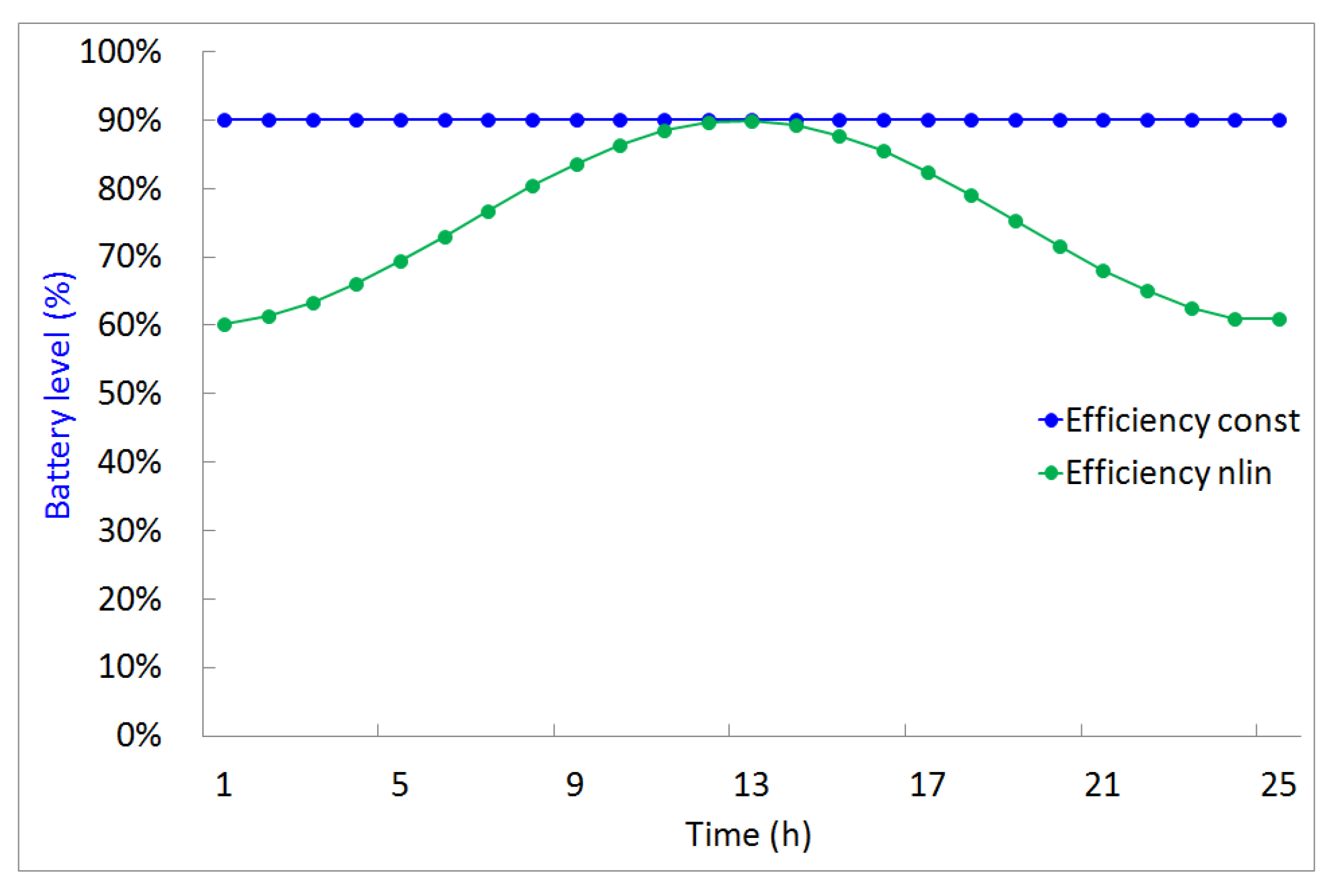
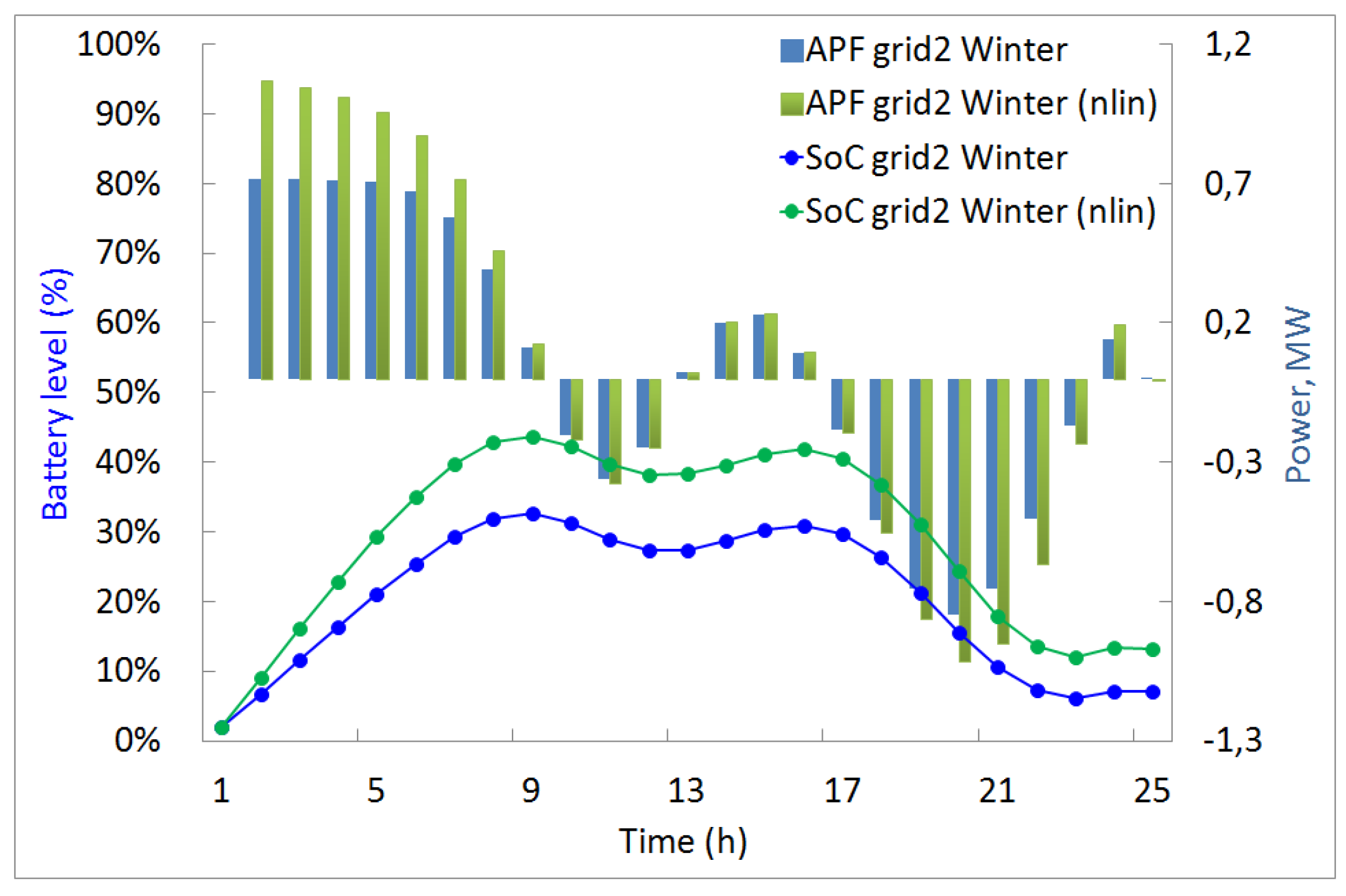
6. Storage System Analysis in Microgrid Using System of Volterra Equations

The proposed approach was tested on real annual climatological and load datasets from the resort village of Goryachinsk, located on the coast of Lake Baikal (Eastern Siberia, Russia). A more detailed description of the real data and 11 years of meteorological observations is shown in [24]. The historical datasets include mean hourly wind speed and time series of direct normal solar irradiance as well as typical electrical load profiles for a selected location. Based on this real dataset, we examined an isolated AC/DC network for one of the four resort villages. This isolated network uses three PVs ($2\times 120$ MW, 33 MW), two wind turbines (220 MW, 186 MW), two hydrogen storages ($2\times 11$ MW), two diesel generators ($2\times 20$ MW) and four batteries ($2\times 150$ MWh, 300 MWh, 180 MWh). The methodology developed in [22,23] let us consider the problem of storage system balancing problem within the hybrid network operational control approach developed in [24] for hybrid AC/DC power systems with renewable energy sources and four storages. As it was outlined in [22], the Volterra integral models can effectively describe the charge–discharge process of energy storage system. The direct problem

$$SOC\left(t\right)=SOC\left(0\right)+{\int }_0^t\mu (·)i\left(\tau \right)d\tau$$

is a well known ampere-hour integral model. The latter is considered as an inverse problem in terms of VIE (or system of VIEs in general setup) with respect to the instantaneous storage current $i\left(\tau \right)$ which is assumed to be positive for charge and negative for discharge. Here $\mu \left(\tau \right)$ is the storage efficiency which can be function of state of charge (SOC) in turn.

For a community of microgrids (MGs) with storage systems, it is useful (see [24] for more details) to employ the following system of Volterra integral equations with jump discontinuous kernels with constrains. Here, we follow notations from [24].

$$\underset{0}{\overset{t}{\int }}\left(\begin{array}{ccc}{K}_{1,1}(t,\tau )& \cdots & K_{1,m}(t,\tau )\\ \cdots & \cdots & \cdots \\ K_{m,1}(t,\tau )& \cdots & K_{m,m}(t,\tau )\end{array}\right)\left(\begin{array}{c}{x}_1\left(\tau \right)\\ ⋮\\ x_m\left(\tau \right)\end{array}\right)d\tau =\left(\begin{array}{c}{f}_1\left(t\right)\\ ⋮\\ f_m\left(t\right)\end{array}\right),$$

(33)

$$K_{i,j}(t,\tau )=\left\{\begin{array}{c}{K}_{i,j}^1(t,\tau ),\mathrm{if}t,\tau \in m_1\\ ⋮\\ K_{i,j}^n(t,\tau ),\mathrm{if}t,\tau \in m_n\end{array}\right.,$$

$$f_i\left(t\right)=f_{iRES}\left(t\right)+f_{iAC/DC}\left(t\right)-f_{iLoad}\left(t\right),$$

$$v_i\left(t\right):={\int }_0^t{x}_i\left(\tau \right)d\tau ,\underset{t\in [0,T]}{max}{v}_i\left(t\right)\le v_{imax},i=1,2,\cdots ,m,$$

$$E_{imin}\left(t\right)\le {\int }_0^t{v}_i\left(\tau \right)d\tau \le E_{imax}\left(t\right),$$

$$0<{\alpha }_1\left(t\right)<\cdots <{\alpha }_{n-1}\left(t\right)<t,$$

where $m_j=\left\{(t,\tau )\right|{\alpha }_{j-1}\left(t\right)<\tau \le {\alpha }_j\left(t\right)\}$, ${\alpha }_0\left(t\right)=0$, ${\alpha }_n\left(t\right)=t$, $j=1,2,\cdots ,n$. Here, m stands for number of grids; functions ${\alpha }_j\left(t\right)$ show the proportions in which units in storage system are used in each subgrid. Here, n is number of units in storage system for i-th grid; the diagonal elements of the matrix $K_{m\times m}$ shows efficiency of storage system of each grid, the remaining elements of the matrix show at the Local Level the coefficients of power flow from storage systems of other grids; $f_{iRES}\left(t\right)$ is the generation from renewable energy sources (RES); $f_{iLoad}$ is predicted electric load of the community, $f_{iAC/DC}\left(t\right)$ is AC/DC power flow at the centralized level; $v_{imax}$ is maximum speed of the charge for i-th storage; $E_{imin}$ and $E_{imax}$ are constraints on the storage levels. The alternating power function (APF) based on $x_i\left(\tau \right)$ is possible to find for each storage using this model.

Let us consider here the model (33) as follows

$${\int }_0^t\left(\begin{array}{cccc}0.75+0.15\left(\frac{t+94}{4}\right)& 0& 0& 0\\ 0& 0.75+0.15\left(\frac{t+94}{4}\right)& 0& 0\\ 0& 0& 0.75+0.15\left(\frac{t+94}{4}\right)& 0\\ 0& 0& 0& 0.75+0.15\left(\frac{t+94}{4}\right)\end{array}\right)\left(\begin{array}{c}{x}_1\left(\tau \right)\\ x_2\left(\tau \right)\\ x_3\left(\tau \right)\\ x_4\left(\tau \right)\end{array}\right)d\tau =$$

(34)

$$=\left(\begin{array}{c}{f}_1\left(\tau \right)\\ f_2\left(\tau \right)\\ f_3\left(\tau \right)\\ f_4\left(\tau \right)\end{array}\right).$$

Here, kernel models the nonlinear efficiency change caused by the night temperature drop (Figure 1).

In (33), $v_{imax}=3.5MW$ is the limitation on the maximum power with which the storage system in i-th grid can be charged and discharged, $E_{imin}=0\%,E_{imax}=100\%.$

$f_i\left(t\right)$ is the disbalance between generation, losses, power flow and load to be compensated by storage system. The calculated APF and SOC are shown in Figure 2.

As can be noted, the calculation results for the Volterra energy storage model, based on nonlinear equations, allow us to obtain a more accurate value of the state of charge for the energy storage and alternating power function in comparison with the linear Volterra model, which was verified based on the conventional linear model [22].

7. Conclusions

In this article, the efficient numerical methods for solution of the novel class of weakly regular linear and nonlinear systems of Volterra integral equations of the first kind are proposed. The iterative method for the solution of the system of nonlinear Volterra integral equations of the first kind with special jump discontinuous kernels employs the linearization of the integral vector-operator, using the Newton–Kantorovich iterative process. The convergence theorem for the proposed iterative process is formulated. The polynomial collocation method is also proposed to solve such systems. It is to be noted that the CESTAC (Controle et Estimation Stochastique des Arrondis de Calculs) method (see [27]) and the CADNA (Control of Accuracy and Debugging for Numerical Applications) library can be employed to control the rounding error estimation and detects possible numerical instabilities.

The efficiently constructed theory and numerical methods are illustrated in five examples and on the practical problem of microgrids balancing using a storage system. The model can effectively handle the nonlinear change of the storage system efficiency drop. In our future work, we will consider the different scenarios of the dynamic analysis of MGs with biomass-based generation and storage systems when efficiency depends on the desired alternating power functions and state of health degradation.

References

1. Volterra, V. Theory of Functionals and of Integral and Integro-Differential Equations; Dover Publications: Mineola, NY, USA, 1959; Volume 4, 226p. [Google Scholar]
2. Tikhonov, A.N.; Arsenin, V.Y. Solutions of Ill-Posed Problems; Winston: Washington, DC, USA, 1977; 258p. [Google Scholar]
3. Evans, G.C. Integral equation of the second kind with discontinuous kernel. Trans. Am. Math. 1910, 11, 393–413. [Google Scholar] [CrossRef]
4. Anselone, P.M. Uniform approximation theory for integral equations with discontinuous kernels. SIAM J. Numer. Anal. 1967, 4, 245–253. [Google Scholar] [CrossRef]
5. Denisov, A.M.; Lorenzi, A. On a special Volterra integral equation of the first kind. Boll. U.M.I. 1995, 7, 443–457. [Google Scholar]
6. Boikov, I.V.; Tynda, A.N. Approximate solution of nonlinear integral equations of developing systems theory. Differ. Equ. 2003, 39, 1214–1223. [Google Scholar] [CrossRef]
7. Tynda, A.N.; Kudryashova, N.Y. Numerical methods for the problems of nonlinear macroeconomic integral models. Zhurnal SVMO 2017, 19, 79–94. [Google Scholar] [CrossRef] [Green Version]
8. Tynda, A.N. Iterative numerical method for integral models of a nonlinear dynamical system with unknown delay. Proc. Appl. Math. Mech. 2009, 9, 591–592. [Google Scholar] [CrossRef]
9. Hritonenko, N.; Yatsenko, Y. Mathematical Modeling in Economics, Ecology and the Environment, 2nd ed.; Springer: Berlin, Germany, 2013. [Google Scholar]
10. Hritonenko, N.; Yatsenko, Y. Nonlinear integral models with delays: Recent developments and applications. J. King Saud Univ. Sci. 2020, 32, 726–731. [Google Scholar] [CrossRef]
11. Ivanov, D.V.; Khamisov, O.V.; Karaulova, I.V.; Markova, E.V.; Trufanov, V.V. Control of power grid development: Numerical solutions. Autom. Remote Control 2004, 65, 472–482. [Google Scholar] [CrossRef]
12. Botoroeva, M.N.; Bulatov, M.V. Applications and methods for the numerical solution of a class of integral-algebraic equations with variable limits of integration. In Bulletin of Irkutsk State University. Series “Mathematics”; Bulletin of Irkutsk State University: Irkutsk, Russia, 2017; Volume 20, pp. 3–16. [Google Scholar] [CrossRef]
13. Apartsyn, A.S. Nonclassical Linear Volterra Equations of the First Kind, 2nd ed.; Series: Inverse and Ill-Posed Problems Series; Kabanikhin, S.I., Ed.; Walter de Gruyter: Berlin, Germany, 2011; Volume 39. [Google Scholar]
14. Sidorov, D.N. On parametric families of solutions of Volterra integral equations of the first kind with piecewise smooth kernel. Differ. Equ. 2013, 49, 210–216. [Google Scholar] [CrossRef]
15. Markova, E.V.; Sidorov, D.N. On one integral Volterra model of developing dynamical systems. Autom. Remote Control 2014, 75, 413–421. [Google Scholar] [CrossRef]
16. Sidorov, D.N. Solvability of systems of Volterra integral equations of the first kind with piecewise continuous kernels. Russ. Math. 2013, 57, 54–63. [Google Scholar] [CrossRef]
17. Sidorov, N.A.; Sidorov, D.N. On the solvability of a class of Volterra operator equations of the first kind with piecewise continuous kernels. Math. Notes 2014, 96, 811–826. [Google Scholar] [CrossRef]
18. Sidorov, D.N. Generalized solution to the Volterra equations with piecewise continuous kernels. Bull. Malays. Math. Sci. Soc. 2014, 37, 757–768. [Google Scholar]
19. Sidorov, D.N.; Sidorov, N.A. Convex majorants method in the theory of nonlinear Volterra equations. Banach J. Math. Anal. 2012, 6, 1–10. [Google Scholar] [CrossRef]
20. Sidorov, D. Integral Dynamical Models: Singularities, Signals and Control; World Scientific Series on Nonlinear Sciences Series A; Chua, L.O., Ed.; World Scientific Press: Singapore, 2015; Volume 87. [Google Scholar]
21. Sidorov, N.; Sidorov, D.; Sinitsyn, A. Toward General Theory of Differential-Operator and Kinetic Models; World Scientific Series on Nonlinear Sciences Series A; Chua, L.O., Ed.; World Scientific Press: Singapore, 2020; Volume 97. [Google Scholar]
22. Sidorov, D.; Muftahov, I.; Tomin, N.; Karamov, D.; Panasetsky, D.; Dreglea, A.; Liu, F. A dynamic analysis of energy storage with renewable and diesel generation using Volterra equations. IEEE Trans. Ind. Inform. 2019. [Google Scholar] [CrossRef] [Green Version]
23. Sidorov, D.; Tao, Q.; Muftahov, I.; Zhukov, A.; Karamov, D.; Dreglea, A.; Liu, F. Energy balancing using charge/discharge storages control and load forecasts in a renewable-energy-based grids. In Proceedings of the 38th China Control Conference, Guangzhou, China, 27–30 July 2019; IEEE: New York, NY, USA, 2019. [Google Scholar] [CrossRef] [Green Version]
24. Sidorov, D.; Panasetsky, D.; Tomin, N.; Karamov, D.; Zhukov, A.; Muftahov, I.; Dreglea, A.; Liu, F.; Li, Y. Toward zero-emission hybrid AC/DC power systems with renewable energy sources and storages: A case study from lake Baikal region. Energies 2020, 13, 1226. [Google Scholar] [CrossRef] [Green Version]
25. Muftahov, I.; Tynda, A.; Sidorov, D. Numeric solution of Volterra integral equations of the first kind with discontinuous kernels. J. Comput. Appl. Math. 2017, 313, 119–128. [Google Scholar] [CrossRef]
26. Kantorovich, L.V.; Akilov, G.P. Functional Analysis, 2nd ed.; Pergamon: Oxford, UK, 1982; 589p. [Google Scholar]
27. Noeiaghdam, S.; Sidorov, D.; Sizikov, V.; Sidorov, N. Control of accuracy on Taylor-collocation method to solve the weakly regular Volterra integral equations of the first kind by using the CESTAC method. Appl. Comput. Math. 2020, 19, 87–105. [Google Scholar]
Figure 1. 24 h efficiency changeover: blue line: constant; green line: nonlinear effect caused by temperature drop.
Mathematics 08 01257 g001
Figure 2. Alternating power functions (APF in MW) with state of charge information (SOC in %) computed by the system of Volterra integral Equation (34) for the winter period.
Mathematics 08 01257 g002