A Simple Parallel Solution Method for the Navier–Stokes Cahn–Hilliard Equations

Abstract

We present a discretization method of the Navier–Stokes Cahn–Hilliard equations which offers an impressing simplicity, making it easy to implement a scalable parallel code from scratch. The method is based on a special pressure projection scheme with incomplete pressure iterations. The resulting scheme admits solution by an explicit Euler method. Hence, all unknowns decouple, which enables a very simple implementation. This goes along with the opportunity of a straightforward parallelization, for example, by few lines of Open Multi-Processing (OpenMP) or Message Passing Interface (MPI) routines. Using a standard benchmark case of a rising bubble, we show that the method provides accurate results and good parallel scalability.

1. Introduction

Phase-field (or diffuse-interface) models have become a valuable tool for the numerical simulation of two-phase flows. In many fields these methods have been proven advantageous compared to traditional sharp interface methods (e.g., Level-Set, Arbitrary Lagrangian–Eulerian, Volume-Of-Fluid). Phase field methods can easily handle (i) moving contact lines (e.g., [1]), (ii) topological transitions (e.g., [2,3]), and (iii) additional chemical species in the fluid and on the interface (e.g., [4]). Further, these methods are relatively robust and do not require additional stabilization techniques such as reinitialization or convection stabilization. It has been shown in recent years that phase field models can be computationally cheap [5] and accurate [6,7] depending on the simulated problem.

Mathematically, phase field methods for two-phase flow are typically described by the Navier–Stokes Cahn–Hilliard equations. Efficient techniques have been proposed for their discretization in space (e.g., [8]) and in time (e.g., [5,9,10]). Due to the necessary high resolution at the fluid–fluid interface, typical discretizations are based on adaptive finite element methods which comes along with a complexity that makes implementations from scratch almost impossible. In addition, the scalable parallelization of such methods is typically challenging and requires a solid knowledge on memory-distributed matrices and vectors and parallel preconditioning and solution techniques. However, given the current shift from serial towards parallel computing, parallelizability is the key component of future numerical algorithms. The goal of this paper is to combine parallelizability with simplicity in a single numerical method. Therefore, we propose a parallel finite difference scheme for the Navier–Stokes Cahn–Hilliard equations.

A finite difference scheme is arguably the simplest way to discretize partial differential equations in space. Efficient finite difference schemes have been proposed for phase field methods, e.g., in [2,3]. Recently, the method has been extended to feature mass conservation and energy stability [11]. All these approaches are rather difficult to understand for a novice and complicated to parallelize as they all involve solvers for coupled systems of equations. Parallel implementations from scratch usually require several thousand lines of code.

Here we aim to avoid the solution of (non-)linear systems of equations by employment of an explicit (forward) Euler method. In this case all unknowns decouple, no system of equations needs to be assembled, and all degrees of freedom can be directly computed from values of the previous time step. This enables straightforward parallelization by few lines of Open Multi-Processing (OpenMP) or Message Passing Interface (MPI) routines. We make this explicit time discretization applicable to these equations of saddle-point structure by a special pressure projection scheme with incomplete pressure iterations. It is known that explicit Euler methods introduce strong time step restrictions of the form $dt<C{h}^2$ for a second order equation and $dt<C{h}^4$ for a fourth order equation, such as the Cahn–Hilliard equation. However, we will show that in practice these restrictions are much less severe and that our proposed method is very efficient as the number of computations per time step is low.

Accordingly, we develop a parallel solution method for the Navier–Stokes equations which can be understood and implemented even for a novice within a few days. We share the (short) code attached to this publication and expect it to be valuable for PhD students and numerical analysts who want to have an easy-to-understand code basis at hand to solve two-phase flow problems with a fast parallel method. Using a standard benchmark case of a rising bubble, we show that our method can provide accurate results in a highly efficient, yet very simple, parallel implementation.

The structure of the remaining paper is as follows. In Section 2 we present the Navier–Stokes Cahn–Hilliard equations. In Section 3 and Section 4, we present the time and space discretization, respectively. The resulting method is challenged in a standard two-phase flow benchmark in Section 5. Afterwards we give some comments on the attached implementation of the method in Section 6. Finally, conclusions are drawn in Section 7.

2. Navier–Stokes Cahn–Hilliard Equations for Two-Phase Flow

The phase field method was originally developed to model solid–liquid phase transitions, see, e.g., [12,13,14]. The interface is represented as a thin layer of finite thickness $\epsilon$ and an auxiliary function, the phase field $\varphi$, is used to indicate the phases. The phase field function varies smoothly between distinct values in both phases and the interface can be associated with an intermediate level set of the phase field function. Diffuse interface approaches for mixtures of two immiscible, incompressible fluids lead to the Navier–Stokes Cahn–Hilliard equations and have been considered by several authors, see, e.g., [8,15,16,17]. If variable (phase-dependent) densities are involved, different formulations of the model equations have been proposed [17,18,19,20]. However, in real scenarios away from the critical point, the involved interface thickness $\epsilon$ is small such that all these models yield comparable results [6]. Therefore, we use the simplest model which reads [17]

$$\begin{array}{ccc}\hfill \rho \left(\varphi \right)\left({\partial }_t\mathbf{u}+(\mathbf{u}·\nabla )\mathbf{u}\right)& =& -\nabla p+\nabla ·\left(\eta \left(\varphi \right)D\left(\mathbf{u}\right)\right)+\mathbf{f}+\tilde{\sigma }{\epsilon }^{-1}\mu \nabla \varphi ,\hfill \end{array}$$

(1)

$$\begin{array}{ccc}\hfill \nabla ·\mathbf{u}& =& 0,\hfill \end{array}$$

(2)

$$\begin{array}{ccc}\hfill {\partial }_t\varphi +\mathbf{u}·\nabla \varphi & =& m\Delta \mu ,\hfill \end{array}$$

(3)

$$\begin{array}{ccc}\hfill \mu & =& {\varphi }^3-\varphi -{\epsilon }^2\Delta \varphi ,\hfill \end{array}$$

(4)

in the domain $\Omega$. Here $\mathbf{u}$, p, $\varphi$, and $\mu$ are the velocity, pressure, phase field variable, and chemical potential, respectively. The parameter m is a mobility constant, $\epsilon$ defines a length scale over which the interface is smeared out. Furthermore, $D\left(\mathbf{u}\right)=\nabla \mathbf{u}+\nabla {\mathbf{u}}^T$ is the (doubled) viscous rate of strain tensor, $\rho \left(\varphi \right)$, $\eta \left(\varphi \right)$, and $\mathbf{f}$ are the (phase dependent) density, viscosity, and body force. The polynomial ${\varphi }^3-\varphi$ arises as the first derivative of the double well potential $W\left(\varphi \right)=1/4{({\varphi }^2-1)}^2$ with respect to $\varphi$. This choice of the polynomial leads to the values $\varphi \approx \pm 1$ in two distinct fluid phases. The parameter $\tilde{\sigma }$ is a scaled surface tension which is a multiple of the physical surface tension $\sigma$. For the given double-well potential, the relation $\tilde{\sigma }=\sigma \frac{3}{2\sqrt{2}}$ holds [21].

Since the solution of the Cahn–Hilliard equation does not satisfy a maximum principle, we follow the approach in [22] and use a truncated phase field function

$$\begin{array}{c}\hfill \widehat{\varphi }=\left\{\begin{array}{cc}\varphi ,\hfill & \left|\varphi \right|\le 1,\hfill \\ \mathrm{sign}\left(\varphi \right),\hfill & \left|\varphi \right|>1,\hfill \end{array}\right.\end{array}$$

(5)

to construct linear interpolations of the viscosity $\eta$ and density $\rho$,

$$\begin{array}{cc}\hfill \eta \left(\varphi \right)& =\frac{\widehat{\varphi }+1}{2}({\eta }_{+1}-{\eta }_{-1})+{\eta }_{-1},\hfill \end{array}$$

(6)

$$\begin{array}{cc}\hfill \rho \left(\varphi \right)& =\frac{\widehat{\varphi }+1}{2}({\rho }_{+1}-{\rho }_{-1})+{\rho }_{-1},\hfill \end{array}$$

(7)

where ${\eta }_{\pm 1}$ and ${\rho }_{\pm 1}$ denote the viscosity and density in the fluid phases where the phase field is $\pm 1$, respectively. Similar truncated phase field functions have played an essential role in the simulation of multi-agent systems [23].

3. Time Discretization

In this section we adopt the explicit Euler scheme for the time discretization of the Navier–Stokes Cahn–Hilliard equations. Let the time interval $[0,T]$ be divided in N subintervals of size $dt$, such that $t^n:=n·dt$, where the upper index denotes the time step number.

Before applying the time discretization to the individual systems we use an operator splitting approach to decouple the Navier–Stokes equations from the Cahn–Hilliard equations. To be more precise, both problems are solved subsequently in every time step. First, we solve the Navier–Stokes system using the values of $\varphi$ and $\mu$ from the previous time step. Then we solve the Cahn–Hilliard system using the just computed velocity field.

3.1. Time Discretization of the Navier–Stokes Equations

The main difficulty in numerically solving the Navier–Stokes equations is that the pressure field is coupled indirectly to the velocity by the incompressibility condition. Chorin [24] and Temam [25] proposed an effective way to decouple the pressure from the velocity by a projection type scheme. As their original scheme has poor accuracy in time many improved versions of these schemes have been introduced since, for details we refer to the review article [26]. Keeping in mind that we aim for an explicit time discretization which enforces small time steps, the time stepping error of the original scheme becomes less important.

In terms of simplicity, the original scheme of Chorin [24] and Temam [25] surpassed all its succeeding versions. The idea is to decouple the momentum and mass balance equations. To this end, an intermediate velocity field ${\tilde{\mathbf{u}}}^{n+1}$ is computed, which satisfies the momentum balance (without the pressure term), but is not divergence-free. Then this field is projected to the space of divergence free functions to obtain the velocity ${\mathbf{u}}^{n+1}$. The latter step involves to first solve an additional equation for the pressure field $p^{n+1}$ which is then used to update the velocity field. Combined with an explicit time discretization the scheme reads:

$$\begin{array}{cc}\hfill \rho \left(\frac{{\tilde{\mathbf{u}}}^{n+1}-{\mathbf{u}}^n}{dt}+\left({\mathbf{u}}^n·\nabla \right){\mathbf{u}}^n\right)& =\nabla ·\left(\eta D\left({\mathbf{u}}^n\right)\right)+{\mathbf{f}}^n+\frac{\tilde{\sigma }}{\epsilon }{\mu }^n\nabla {\varphi }^n,\hfill \end{array}$$

(8)

$$\begin{array}{cc}\hfill \nabla ·\left(\frac{1}{\rho }\nabla p^{n+1}\right)& =\frac{\nabla ·{\tilde{\mathbf{u}}}^{n+1}}{dt},\frac{\partial p^{n+1}}{\partial n}|\partial \Omega =0,\hfill \end{array}$$

(9)

$$\begin{array}{cc}\hfill \rho \frac{{\mathbf{u}}^{n+1}-{\tilde{\mathbf{u}}}^{n+1}}{dt}& =-\nabla p^{n+1},\hfill \end{array}$$

(10)

where $\partial /\partial n$ denotes the normal derivative on the domain boundary $\partial \Omega$.

Equations (8)–(10) are decoupled and can be solved subsequently. The first equation is used to compute an intermediate (not divergence-free) velocity field ${\tilde{\mathbf{u}}}^{n+1}$. The second equation computes the pressure which is then used to obtain a divergence-free velocity field ${\mathbf{u}}^{n+1}$ from the last equation. Hence, Equations (9) and (10) can be seen as the projection of ${\tilde{\mathbf{u}}}^{n+1}$ onto the space of divergence-free vector fields.

The first and third equation are completely explicit, i.e., the sought variables ${\tilde{\mathbf{u}}}^{n+1}$ and ${\mathbf{u}}^{n+1}$ can be directly computed. The second equation is a Poisson equation and is usually handled by assembling a matrix which can be solved with the conjugate gradient method or by shifting the problem to Fourier space and solving with spectral methods.

Again, as we aim for simplicity we follow a different approach here. The idea is to make Equation (9) amenable to an explicit Euler method by including a time derivative of the pressure. In fact, the solution $p^{n+1}$ from Equation (9) can be seen as the stationary solution of the convergent heat equation

$${\partial }_{t}p-\nabla ·\left(\frac{1}{\rho }\nabla p\right)=-\frac{\nabla ·{\tilde{\mathbf{u}}}^{n+1}}{dt},\frac{\partial p^{n+1}}{\partial n}|\partial \Omega =0.$$

Instead of solving this equation exactly, we propose to solve only K steps of the time evolution by an explicit Euler scheme. Accordingly, we introduce $K-1$ intermediate values $p^{n+k/K}$ for $k=1,\dots ,K-1$ which can be computed successively from

$$\begin{array}{cc}\hfill \frac{p^{n+\frac{k+1}{K}}-p^{n+\frac{k}{K}}}{\widetilde{dt}}-\nabla ·\left(\frac{1}{\rho }\nabla p^{n+\frac{k}{K}}\right)& =-\frac{\nabla ·{\tilde{\mathbf{u}}}^n}{dt},k=0,\dots K-1,\hfill \end{array}$$

(11)

with a different time step size $\widetilde{dt}$. As we aim for the stationary solution it is desired to choose $\widetilde{dt}$ as large as possible. From the explicit Euler scheme, the time step restriction $\widetilde{dt}<\rho h^2/4$ emerges. To be well below this barrier, we use half of this time step size, $\widetilde{dt}=\rho h^2/8$, throughout this work.

As the time step size of the overall projection method, $dt$, is small, we can expect that the velocity and pressure change only slightly in every time step. Hence, very few iterations K of Equation (11) should suffice to update the pressure. In the simplest case, $K=1$, Equation (11) reduces to a direct computation of $p^{n+1}$ by

$$\begin{array}{cc}\hfill \frac{p^{n+1}-p^n}{\widetilde{dt}}-\nabla ·\left(\frac{1}{\rho }\nabla p^n\right)& =-\frac{\nabla ·{\tilde{\mathbf{u}}}^n}{dt}.\hfill \end{array}$$

This choice can be sufficient if the time step size is small enough.

3.2. Time Discretization of the Cahn–Hilliard Equations

The explicit Euler scheme for the Cahn–Hilliard equation reads

$$\begin{array}{cc}\hfill & \frac{{\varphi }^{n+1}-{\varphi }^n}{dt}+{\mathbf{u}}^{n+1}·\nabla {\varphi }^n=m\Delta {\mu }^n,\hfill \end{array}$$

(12)

$$\begin{array}{cc}\hfill & {\mu }^n=-{\epsilon }^2\Delta {\varphi }^n+{\left({\varphi }^n\right)}^3-{\varphi }^n.\hfill \end{array}$$

(13)

Due to the explicit presence of a fourth order space derivative, a time step restriction arises: $dt<C{h}^4/\left(m{\epsilon }^2\right)$. Luckily, this restriction turns out to be less severe after the following considerations. Firstly, the interface length $\epsilon$ is very small. The real thickness of a fluid–fluid interface is in the order of nanometers, unless the temperature is close to the critical point. This length scale cannot be resolved in numerical methods as soon as the length scale of the problem exceeds the micrometer range. Hence, in any useful numerical approximation that aims to be close to the real physical solution, $\epsilon$ is chosen as small as possible. In practice, that means $\epsilon$ is chosen similar to the grid size, $\epsilon \approx h$. Consequently, the above time step restriction effectively reduces to $dt<C{h}^2/m$. This condition is weakened further, as m is typically very small. The interface moves physically with the fluid velocity, thus m needs to be so small that the right-hand side of Equation (12) hardly moves the interface but only conserves the interface shape, similar to reinitialization in Level-Set methods. In addition, matched asymptotic analysis shows the convergence of diffuse-interface methods toward the sharp interface equations only for small CH mobility [20].

The remaining time step restriction can be tolerated, given that the number of computations in each time step is relatively low in comparison to implicit time discretization methods. While the latter reduces time step restrictions, they typically involve several orders more computations per time step, due to the necessary solution of a (linear) system of equations, which is avoided in our method.

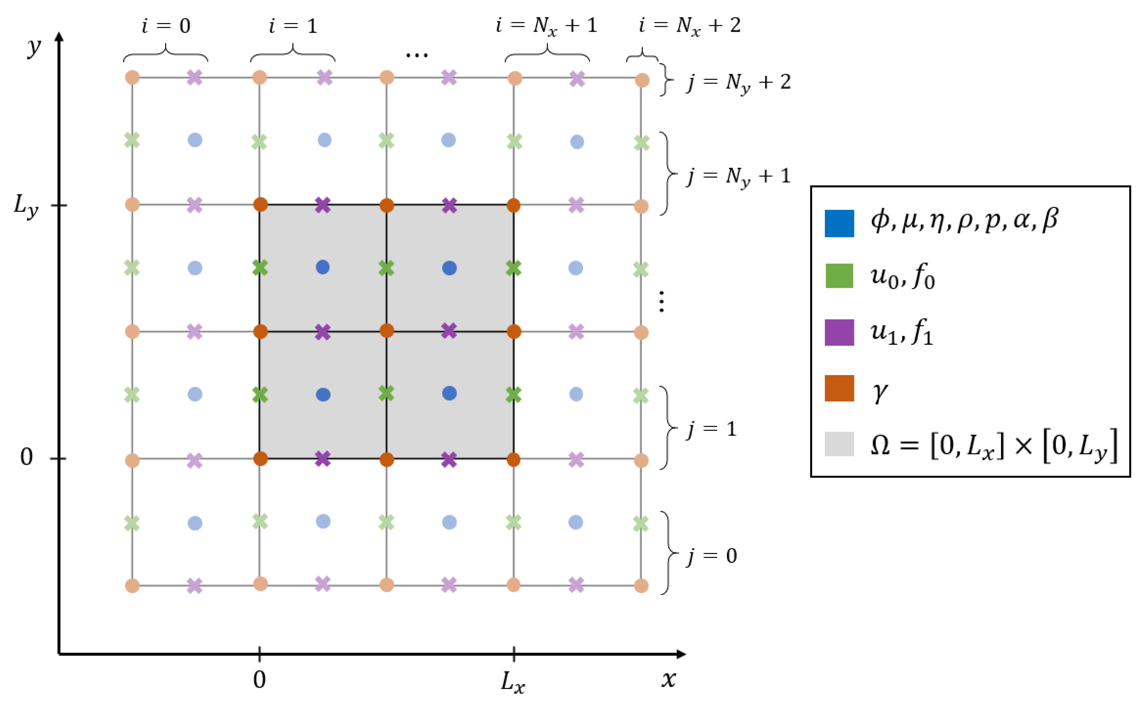
4. Space Discretization

The time discrete scheme presented in the previous section is discretized in space by a finite difference method. We use an equidistant rectangular grid with equal spacing h in all directions. For simplicity the following discussion is restricted to two dimensions, but we note that the scheme can be easily extended to three dimensions. The rectangular computational domain $\Omega =[0,L_x]\times [0,L_y]$ is subdivided into $N_x·N_y$ square cells with $N_x=L_x/h,N_y=L_y/h$.

Scalar variables are defined in the centers of these cells. One additional layer of ghost points is included outside of each boundary facet. To stay close to the implementation we use only integer indices to describe the values of all variables on the grid points. Hence, the discrete grid values of a scalar field $q(x,y)$ are defined as

$$\begin{array}{ccc}\hfill q_{i,j}& =q\left(\left(i-\frac{1}{2}\right)h,\left(j-\frac{1}{2}\right)h\right),\hfill & \hfill i=0,\dots ,N_x+1,j=0,\dots ,N_y+1,\end{array}$$

where q is a placeholder for $\varphi ,\mu ,p$.

To avoid spatial oscillations from the odd-even decoupling between pressure and velocity, a staggered Cartesian grid is employed [27]. On a staggered grid the velocity variables $(u_0,u_1)=:\mathbf{u}$ are shifted by $h/2$ in their respective direction to the cell faces. Figure 1 shows the arrangement of all the different variables on the grid. To stay close to the implementation we use only integer indices to describe the values of all variables on the grid points:

$$\begin{array}{ccc}\hfill u_{0_{i,j}}& =u_0\left(\left(i-1\right)h,\left(j-\frac{1}{2}\right)h\right),\hfill & \hfill i=0,\dots ,N_x+2,j=0,\dots ,N_y+1,\\ \hfill u_{1_{i,j}}& =u_1\left(\left(i-\frac{1}{2}\right)h,\left(j-1\right)h\right),\hfill & \hfill i=0,\dots ,N_x+1,j=0,\dots ,N_y+2.\end{array}$$

Note, that ghost points are also included for the velocity field. While this might not be necessary, depending on the boundary condition, it simplifies and unifies indexing and implementation at negligible additional memory consumption.

We introduce for some quantity q the discrete Laplacian ${\Delta }_h$, all-sided average A, horizontal and vertical averages $A_x,A_y$, backward differences $D_x,D_y$, and central differences $D_{2x},D_{2y}$ as follows:

$$\begin{array}{c}\hfill \begin{array}{ccc}\hfill & \hfill {\Delta }_h{q}_{i,j}& :=(q_{i+1,j}+q_{i-1,j}+q_{i,j+1}+q_{i,j-1}-4q_{i,j})/h^2,\hfill \\ \hfill & \hfill A{q}_{i,j}& :=(q_{i,j}+q_{i-1,j}+q_{i,j-1}+q_{i-1,j-1})/4,\hfill \end{array}\\ \hfill \begin{array}{cccc}\hfill A_x{q}_{i,j}& :=(q_{i,j}+q_{i-1,j})/2,\hfill & \hfill A_y{q}_{i,j}& :=(q_{i,j}+q_{i,j-1})/2,\hfill \\ \hfill D_x{q}_{i,j}& :=(q_{i,j}-q_{i-1,j})/h,\hfill & \hfill D_y{q}_{i,j}& :=(q_{i,j}-q_{i,j-1})/h,\hfill \\ \hfill D_{2x}{q}_{i,j}& :=(q_{i+1,j}-q_{i-1,j})/2h,\hfill & \hfill D_{2y}{q}_{i,j}& :=(q_{i,j+1}-q_{i,j-1})/2h.\hfill \end{array}\end{array}$$

4.1. Matched Densities and Viscosities

In the beginning let us consider the simple case of matched viscosity ($\eta ={\eta }_{-1}={\eta }_{+1}$) and matched density ($\rho ={\rho }_{-1}={\rho }_{+1}$). In this case the viscous stress contribution reduces to $\eta \Delta \mathbf{u}$ and the space discretization of Equation (8) reads

$$\begin{array}{cc}{\tilde{u}}_{0_{i,j}}^{n+1}\hfill & =u_{0_{i,j}}^n-dt{\left({\mathbf{u}}^n·\nabla {\mathbf{u}}^n\right)}_{0_{i,j}}+\frac{dt}{\rho }\left(\eta {\Delta }_h{u}_{0_{i,j}}^n+\frac{\tilde{\sigma }}{\epsilon }{A}_x{\mu }_{i,j}^n·D_x{\varphi }_{i,j}^n+f_{0_{i,j}}^n\right)\hfill \\ \hfill & \mathrm{for}i=2,\dots ,N_x;j=1,\dots ,N_y,\hfill \end{array}$$

(14)

$$\begin{array}{cc}{\tilde{u}}_{1_{i,j}}^{n+1}\hfill & =u_{1_{i,j}}^n-dt{\left({\mathbf{u}}^n·\nabla {\mathbf{u}}^n\right)}_{1_{i,j}}+\frac{dt}{\rho }\left(\eta {\Delta }_h{u}_{1_{i,j}}^n+\frac{\tilde{\sigma }}{\epsilon }{A}_y{\mu }_{i,j}^n·D_y{\varphi }_{i,j}^n+f_{1_{i,j}}^n\right)\hfill \\ \hfill & \mathrm{for}i=1,\dots ,N_x;j=2,\dots ,N_y,\hfill \end{array}$$

(15)

with

$$\begin{array}{cc}\hfill {\left({\mathbf{u}}^n·\nabla {\mathbf{u}}^n\right)}_{i,j}& =\left(\begin{array}{c}{u}_{0_{i,j}}^n{D}_{2x}{u}_{0_{i,j}}^n+A{u}_{1_{i,j+1}}^n{D}_{2y}{u}_{0_{i,j}}^n\\ A{u}_{0_{i+1,j}}^n{D}_{2x}{u}_{1_{i,j}}^n+u_{1_{i,j}}^n{D}_{2y}{u}_{1_{i,j}}^n\end{array}\right).\hfill \end{array}$$

Boundary conditions to the velocity are included in this step as explained in the Appendix A.

After computing ${\tilde{\mathbf{u}}}^{n+1}$ directly from these equations, the pressure $p^{n+1}$ is calculated from the discretized version of Equation (11),

$$\begin{array}{cc}\hfill p_{i,j}^{n+\frac{k+1}{K}}& =p_{i,j}^{n+\frac{k}{K}}+\frac{h^2}{8}{\Delta }_h{p}_{i,j}^{n+\frac{k}{K}}-\frac{\rho h}{8dt}\left({\tilde{u}}_{0_{i+1,j}}^n-{\tilde{u}}_{0_{i,j}}^n+{\tilde{u}}_{1_{i,j+1}}^n-{\tilde{u}}_{1_{i,j}}^n\right)\hfill \\ \hfill & \mathrm{for}i=1,\dots ,N_x;j=1,\dots ,N_y,\hfill \end{array}$$

(16)

which is solved for $k=0,\dots K-1$ to successively compute $p_{i,j}^{n+\frac{1}{K}},p_{i,j}^{n+\frac{2}{K}},\dots ,p_{i,j}^{n+1}$, for a small constant K.

Finally, the new velocity field is computed from

$$\begin{array}{cc}\hfill u_{0_{i,j}}^{n+1}& ={\tilde{u}}_{0_{i,j}}^{n+1}-\frac{dt}{\rho }{D}_x{p}_{i,j}^{n+1}\hfill \\ \hfill & \mathrm{for}i=2,\dots ,N_x;j=1,\dots ,N_y,\hfill \end{array}$$

(17)

$$\begin{array}{cc}\hfill u_{1_{i,j}}^{n+1}& ={\tilde{u}}_{1_{i,j}}^{n+1}-\frac{dt}{\rho }{D}_y{p}_{i,j}^{n+1}\hfill \\ \hfill & \mathrm{for}i=1,\dots ,N_x;j=2,\dots ,N_y.\hfill \end{array}$$

(18)

After calculation of the new velocity, the Cahn–Hilliard system is solved. Using central differences for the advective term, a second order in space discretization of the Cahn–Hilliard Equations (12) and (13) reads

$$\begin{array}{cc}\hfill {\mu }_{i,j}^n& =-{\epsilon }^2{\Delta }_h{\varphi }_{i,j}^n+{\left({\varphi }_{i,j}^n\right)}^3-{\varphi }_{i,j}^n,\hfill \\ \hfill {\varphi }_{i,j}^{n+1}& ={\varphi }_{i,j}^n-dt\left(A_x{u}_{0_{i+1,j}}^{n+1}·D_{2x}{\varphi }_{i,j}^n+A_y{u}_{1_{i,j+1}}^{n+1}·D_{2y}{\varphi }_{i,j}^n\right)+mdt{\Delta }_h{\mu }_{i,j}^n\hfill \\ \hfill & \mathrm{for}i=1,\dots ,N_x;j=1,\dots ,N_y.\hfill \end{array}$$

(19)

The homogeneous Neumann boundary conditions are included as explained in the Appendix A.

Equations (14)–(19) provide a way to directly solve the Navier–Stokes Cahn–Hilliard system. We again note the equations can be solved individually for each i and j, no coupled system of equations is involved. Hence, the solution algorithm can be easily implemented with a few dozen lines of code. Due to the direct calculation, parallelization (e.g., with OpenMP or MPI) is straightforward, can be done with a few lines of code and can be expected to scale very well.

4.2. Non-Matched Density and Viscosity

In the general case of non-matched density and viscosity the discretization becomes more elaborate. We define ${\eta }_{i,j}^n=\eta \left({\varphi }_{i,j}^n\right)$ and ${\rho }_{i,j}^n=\rho \left({\varphi }_{i,j}^n\right)$ and replace $\rho$ in Equations (14) and (17) by $A_x{\rho }_{i,j}^n$ and in Equations (15) and (18) by $A_y{\rho }_{i,j}^n$. Additionally, in Equation (16) we replace $\rho$ by ${\rho }_{i,j}^n$ and ${\Delta }_h{p}_{i,j}^{n+\frac{k}{K}}$ by

$$\begin{array}{cc}\hfill {\left({\rho }^n\nabla ·\left(\frac{1}{{\rho }^n}\nabla p^{n+\frac{k}{K}}\right)\right)}_{i,j}& ={\left(\Delta p^{n+\frac{k}{K}}+{\rho }^n\nabla \frac{1}{{\rho }^n}·\nabla p^{n+\frac{k}{K}}\right)}_{i,j}\hfill \\ \hfill & ={\Delta }_h{p}_{i,j}^{n+\frac{k}{K}}+{\rho }_{i,j}^n\left(D_{2x}\frac{1}{{\rho }_{i,j}^n}·D_{2x}{p}_{i,j}^{n+\frac{k}{K}}+D_{2y}\frac{1}{{\rho }_{i,j}^n}·D_{2y}{p}_{i,j}^{n+\frac{k}{K}}\right).\hfill \end{array}$$

(20)

To deal with non-constant viscosity we introduce the fields $\alpha ,\beta ,\gamma$ to represent the viscous stress,

$$\begin{array}{cc}\hfill \left[\begin{array}{cc}\alpha & \gamma \\ \gamma & \beta \end{array}\right]& :=\eta \left(\nabla \mathbf{u}+{(\nabla \mathbf{u})}^T\right).\hfill \end{array}$$

In the discrete case, $\alpha$ and $\beta$ are naturally defined in the cell centers, $\gamma$ is defined on the cell vertices. This leads to

$$\begin{array}{cc}\hfill {\alpha }_{i,j}^n& =2{\eta }_{i,j}^n{D}_x{u}_{0_{i+1,j}}^n,\hfill \\ \hfill {\beta }_{i,j}^n& =2{\eta }_{i,j}^n{D}_y{u}_{1_{i,j+1}}^n,\hfill \\ \hfill {\gamma }_{i,j}^n& =\left(D_y{u}_{0_{i,j}}^n+D_x{u}_{1_{i,j}}^n\right)A{\eta }_{i,j}^n.\hfill \end{array}$$

These terms are then used to replace the viscous terms $\eta {\Delta }_h{u}_{0_{i,j}}^n$ and $\eta {\Delta }_h{u}_{1_{i,j}}^n$ in Equations (14) and (15) by $D_x{\alpha }_{i,j}^n+D_y{\gamma }_{i,j+1}^n$ and $D_y{\beta }_{i,j}^n+D_x{\gamma }_{i+1,j}^n$, respectively.

5. Benchmark Test Results

To validate the accuracy of the model, a benchmark test as described by test case 1 in [28] is conducted. This test can be seen as the standard benchmark for two-phase flows and has been conducted for many different numerical methods (e.g., Level-Set, Volume-of-Fluid, Arbitrary Lagrangian–Eulerian). The benchmark was applied to various phase field methods in [6].

5.1. Test Scenario

The test specifies a circular bubble of one fluid (here $\varphi \approx 1$), which rises in a rectangular domain $\Omega =[1,0]\times [2,0]$ filled with another fluid (here $\varphi \approx -1$). The initial position of the center of the bubble is at $(0.5,0.5)$ and its radius is 0.25, which results in the initial condition

$${\varphi }_{i,j}^0=tanh\frac{0.25-\sqrt{{\left(\left(i-0.5\right)·h-0.5\right)}^2-{\left(\left(j-0.5\right)·h-0.5\right)}^2}}{\sqrt{2}\epsilon }$$

(21)

Test case 1 of [28] prescribes for the outer fluid the physical quantities ${\rho }_{-1}=1000$ and ${\eta }_{-1}=10$. The inner fluid of the bubble is defined by ${\rho }_{+1}=100$ and ${\eta }_{+1}=1$. Furthermore, the gravitational force vector is set to $\mathbf{f}=(0,-0.98(\rho \left(\varphi \right)-{\rho }_{-1}))$ and the surface tension $\sigma$ to $24.5$. No slip boundary conditions are specified at the top and bottom, a free slip condition is imposed at the lateral boundaries. Due to the different densities of the inner and outer fluids, the bubble will rise in the vertical tube over time. The simulation is run for 3 time units during which some benchmark quantities are computed.

The chosen four combinations of numerical parameters are listed in

Table 1. Numerical parameters: grid resolution h, diffuse interface width $\epsilon$, and time step size $dt$ and the resulting total degrees of freedom NDOF per time step and average CPU time of each parameter case.

h	$\mathit{\epsilon }$	$\mathbf{dt}$	NDOF	CPU Time [s]
1/32	0.04	64 × 10−5	10,240	37.18
1/64	0.02	16 × 10−5	40,960	132.93
1/128	0.01	4 × 10−5	163,840	717.62
1/256	0.005	1 × 10−5	655,360	5904.87

. Their choice is guided by reported values in the phase field benchmark [6]: The interface thickness $\epsilon$ is refined proportional to grid size h, which keeps the number of elements along the interface fixed.

The mobility is set to a small constant, $m=0.01$, which is by a factor ten higher than the value chosen in [6] (acknowledging the different scaling of mu there). We conducted a preliminary study to determine that this value of m is large enough to keep a good shape of the phase field interface profile while introducing only small (undesired) Cahn–Hilliard diffusion, which is confirmed by the accuracy of the results in Section 5.3. In addition, note that results are essentially independent of m when $ϵ\to 0$, see [20]. Given the previously discussed time step restrictions, the time step size is scaled quadratically with grid size.

Similar to [6], the total number of degrees of freedom per time step is reported for the four different simulations. Additionally, the CPU time of each parameter case is listed in Table 1 for an OpenMP implementation running on four cores.

5.2. Measured Quantities

In order to compare our results with the literature some of the benchmark quantities presented in [28] are used. Their calculation is described below:

(1) Center of Mass

$$\begin{array}{c}\hfill y_c=\frac{{\int }_{\Omega }\left(\varphi +1\right)·y}{{\int }_{\Omega }\left(\varphi +1\right)},\end{array}$$

(2) Rise Velocity

$$\begin{array}{c}\hfill V_c=\frac{{\int }_{\Omega }\left(\varphi +1\right)·u_1}{{\int }_{\Omega }\left(\varphi +1\right)}.\end{array}$$

(3) Error Norms and Orders of Convergence

The following three error norms are also specified in [28] and will be used for the evaluation of our results:

$$\begin{array}{cccccc}\hfill {\parallel e\parallel }_1& =\frac{{\sum }_{n=1}^N|q_{ref}^n-q^n|}{{\sum }_{n=1}^N\left|q_{ref}^n\right|},\hfill & \hfill {\parallel e\parallel }_2& ={\left(\frac{{\sum }_{n=1}^N{|q_{ref}^n-q^n|}^2}{{\sum }_{n=1}^N{\left|q_{ref}^n\right|}^2}\right)}^{0.5},\hfill & \hfill {\parallel e\parallel }_{\infty }& =\frac{{max}_n|q_{ref}^n-q^n|}{{max}_n\left|q_{ref}^n\right|},\hfill \end{array}$$

where $q^n$ is the temporal evolution of quantity q. We use the results of the simulation with the finest grid and smallest time steps as the reference solution $q_{ref}^n$. Spline interpolation is used to match the time steps of the reference solution with our solution. Using the so defined errors, a rate of convergence (ROC) can be computed as follows:

$$\begin{array}{c}\hfill ROC=log\left(\frac{{\mathrm{error}}_{2h}}{{\mathrm{error}}_h}\right)/log\left(2\right),\end{array}$$

where ${\mathrm{error}}_h$ denotes the error as defined above on a grid of grid size h.

5.3. Results

5.3.1. Bubble Shape

As already described in [28], the initial circular bubble changes its shape over time to an ellipsoidal shape. In Figure 2 one can see the different bubble shapes at the end time $t=3$ compared to the reference results from group 1 in [28]. It shows that the shapes of our model approximate the reference solution as grid resolution and interface thickness are refined. Especially the final bubble shapes of the two finest grids with $h=1/128$ and $h=1/256$ got very close to the reference results, as they are wider than the bubble shapes produced by the other two simulations.

5.3.2. Benchmark Quantities

In addition to the bubble shapes, we evaluated different benchmark quantities as defined before. Figure 3 shows the center of mass and the rise velocity of the bubble over time in comparison to the reference solution from [28].

Both measured quantities approach the reference values with increasing grid resolutions. In the “eye norm” the center of mass is nearly identical for the two finest grids, while the simulation with $h=1/32$ is more off. Differences between the parameter cases are more pronounced when looking at the rise velocity. Here, one can see more clearly that all curves approach the reference solution with increasing grid resolutions. This behavior is also confirmed in

Table 2. Benchmark quantities: Maximum rise velocity $V_{c,max}$ with corresponding time ${t|}_{V_c=V_{c,max}}$ and final position of the center of mass $y_c(t=3)$ with reference results from group 1 in [28].

(h)	${\mathit{V}}_{\mathit{c},\mathit{max}}$	${\mathit{t}|}_{{\mathit{V}}_{\mathit{c}}={\mathit{V}}_{\mathit{c},\mathit{max}}}$	${\mathit{y}}_{\mathit{c}}(\mathit{t}=3)$
1/32	0.2081	1.0630	1.0329
1/64	0.2295	0.9730	1.0654
1/128	0.2372	0.9420	1.0753
1/256	0.2395	0.9270	1.0776
ref	0.2417	0.9213	1.0813

which lists the maximum rise velocity and the final center of mass. A comparison with the phase field results from [6] reveals similarly small deviations from the reference solutions in [28] which indicates that these differences stem mostly from the modeling error due to non-zero interface thickness.

5.3.3. Error Norms

Finally, the calculated error norms and the resulting orders of convergence are presented in

Table 3. Error norms and orders of convergence.

h	${\left|\right|\mathit{e}\left|\right|}_1$	${\mathit{ROC}}_1$	${\left|\right|\mathit{e}\left|\right|}_2$	${\mathit{ROC}}_2$	${\left|\right|\mathit{e}\left|\right|}_{\mathit{\infty }}$	${\mathit{ROC}}_3$
Center of mass
1/32	0.0387		0.0423		0.0415
1/64	0.0116	1.7435	0.0125	1.7525	0.0119	1.8090
1/128	0.0025	2.1930	0.0027	2.2039	0.0025	2.2164
Rise velocity
1/32	0.1121		0.1173		0.1609
1/64	0.0351	1.6765	0.0370	1.6655	0.0531	1.5998
1/128	0.0081	2.1143	0.0087	2.0940	0.0130	2.0256

. Overall, the previous observations are confirmed, since all the calculated errors become smaller with finer grid resolutions and shorter time step lengths. The ROC values indicate clear second order convergence for all error norms. Note that this implies second order convergence in space and first order in time as time step size is scaled quadratically with the grid size.

5.3.4. Parallelization

Finally, we tested the model for different numbers of cores to examine the parallel efficiency. The resulting time measurements and calculated speedup can be found in Figure 4. Here, the dimensions of the field were $512\times 1024$ grid points and the number of time steps was set to 3000. It can be seen that the implementation of the proposed discretization method is highly parallelizable leading to a nearly perfect linear speedup. It is noteworthy that parallelization has been achieved by a few simple OpenMP ’parallel for’ directives. Given the problem size is large enough, a similarly good linear speedup can also be expected for much larger number of cores, for OpenMP as well as MPI parallelization.

6. Implementation

We share the code in the supporting material attached to this publication and additionally on GitHub: https://github.com/soranad-a/parallel-navier-stokes-cahn-hilliard. It contains the discretized Navier–Stokes Cahn–Hilliard system implemented in C++, whereby the variable names were kept analogous to those in the equations above. Furthermore, the code includes OpenMP for parallelization on multiple cores. It consists of the following three files:

• helpers.h—handles output and data structure of 2 dimensional arrays.
• config.conf—self explanatory file defining all constants and simulation parameters.
• main.cc—contains core code of the numerical algorithm, but most of the lines are needed for reading parameters and managing output.

The code can be compiled by: g++ -std=c++17 -fopenmp -O3 main.cc.

To enable the correct output of the simulation files, the program needs a subfolder named paraview/into which it writes its output files, which can be visualized in the open-source data analysis software ParaView (www.paraview.org). Furthermore, during runtime, a file named benchmark.csv is created, which contains the measured benchmark quantities.

7. Conclusions

We have presented a discretization method of the Navier–Stokes Cahn–Hilliard equations. The method offers an impressing simplicity, which is based on an explicit Euler time discretization of a special pressure projection scheme with incomplete pressure iterations. Hence, it is not necessary to solve a linear system of equations as all unknowns decouple, and computations can be done separately for each grid point. Consequently, the method can be easily implemented from scratch and parallelization is straightforward by few lines of OpenMP or MPI routines.

A standard benchmark case of a rising bubble is used to evaluate the method in practice. We find that the arising time step restrictions are not critical as the number of compute instructions per time step is relatively low. We show that the method provides accurate solutions comparable to previous results from finite-element methods [6,28]. The numerical results approach reference values as grid size and interface thickness are decreased. The computed ROC indicates second order convergence. Finally, we measure computation time for up to 24 CPU cores and find a nearly perfect parallel speedup.

We share the (short) code attached to this publication and expect it to be valuable for novices in phase field simulations who want to have an easy-to-understand code basis at hand to solve two-phase flow problems with a fast parallel method. The method is flexible and can easily be augmented to account for additional physical processes. In the future we plan to extend the method to describe flows in complex evolving geometries [29] and fluid-structure interaction using the approach in [30]. We further address the large-scale parallelization by use of GPUs.

References

1. Aland, S.; Chen, F. An efficient and energy stable scheme for a phase-field model for the moving contact line problem. Int. J. Numer. Methods Fluids 2016, 81, 657–671. [Google Scholar] [CrossRef]
2. Kim, J. Phase-Field Models for Multi-Component Fluid Flows. Commun. Comput. Phys. 2012, 12, 613–661. [Google Scholar] [CrossRef]
3. Lee, H.G.; Kim, J. An efficient numerical method for simulating multiphase flows using a diffuse interface model. Phys. A Stat. Mech. Appl. 2015, 423, 33–50. [Google Scholar] [CrossRef]
4. Aland, S. Phase field models for two-phase flow with surfactants and biomembranes. In Transport Processes at Fluidic Interfaces; Springer: Cham, Switzerland, 2017; pp. 271–290. [Google Scholar]
5. Aland, S. Time integration for diffuse interface models for two-phase flow. J. Comput. Phys. 2014, 262, 58–71. [Google Scholar] [CrossRef] [Green Version]
6. Aland, S.; Voigt, A. Benchmark computations of diffuse interface models for two-dimensional bubble dynamics. Int. J. Numer. Methods Fluids 2012, 69, 747–761. [Google Scholar] [CrossRef]
7. Aland, S.; Boden, S.; Hahn, A.; Klingbeil, F.; Weismann, M.; Weller, S. Quantitative comparison of Taylor flow simulations based on sharp-interface and diffuse-interface models. Int. J. Numer. Methods Fluids 2013, 73, 344–361. [Google Scholar] [CrossRef]
8. Kay, D.; Welford, R. Efficient Numerical Solution of Cahn-Hilliard-Navier-Stokes Fluids in 2D. SIAM J. Sci. Comput. 2007, 29, 2241–2257. [Google Scholar] [CrossRef]
9. Han, D.; Wang, X. A second order in time, uniquely solvable, unconditionally stable numerical scheme for Cahn–Hilliard–Navier–Stokes equation. J. Comput. Phys. 2015, 290, 139–156. [Google Scholar] [CrossRef] [Green Version]
10. Shen, J.; Yang, X. Decoupled, energy stable schemes for phase-field models of two-phase incompressible flows. SIAM J. Numer. Anal. 2015, 53, 279–296. [Google Scholar] [CrossRef]
11. Guo, Z.; Lin, P.; Lowengrub, J.; Wise, S.M. Mass conservative and energy stable finite difference methods for the quasi-incompressible Navier–Stokes–Cahn–Hilliard system: Primitive variable and projection-type schemes. Comput. Methods Appl. Mech. Eng. 2017, 326, 144–174. [Google Scholar] [CrossRef] [Green Version]
12. Anderson, D.; McFadden, G.; Wheeler, A. Diffuse interface methods in fluid mechanics. Ann. Rev. Fluid Mech. 1998, 30, 139–165. [Google Scholar] [CrossRef] [Green Version]
13. Emmerich, H. Advances of and by phase-field modeling in condensed-matter physics. Adv. Phys. 2008, 57, 1–87. [Google Scholar] [CrossRef]
14. Singer-Loginova, I.; Singer, H. The phase field technique for modeling multiphase materials. Rep. Prog. Phys. 2008, 71, 106501. [Google Scholar] [CrossRef] [Green Version]
15. Jaqmin, D. Calculation of two-phase Navier-Stokes flows using phase-field modelling. J. Comput. Phys. 1999, 155, 96–127. [Google Scholar] [CrossRef]
16. Feng, X. Fully Discrete Finite Element Approximations of the Navier–Stokes–Cahn-Hilliard Diffuse Interface Model for Two-Phase Fluid Flows. SIAM J. Numer. Anal. 2006, 44, 1049–1072. [Google Scholar] [CrossRef]
17. Ding, H.; Spelt, P.; Shu, C. Diffuse interface model for incompressible two-phase flows with large density ratios. J. Comput. Phys. 2007, 226, 2078–2095. [Google Scholar] [CrossRef]
18. Boyer, F. A theoretical and numerical model for the study of incompressible mixture flows. Comput. Fluids 2002, 31, 41–68. [Google Scholar] [CrossRef] [Green Version]
19. Lowengrub, J.; Truskinovsky, L. Quasi-incompressible Cahn-Hilliard fluids and topological changes. Proc. Roy. Soc. Lond. A 1998, 454, 2617–2654. [Google Scholar] [CrossRef]
20. Abels, H.; Garcke, H.; Grün, G. Thermodynamically consistent, frame indifferent diffuse interface models for incompressible two-phase flows with different densities. Math. Model. Methods Appl. Sci. 2012, 22, 1150013. [Google Scholar] [CrossRef]
21. Aland, S. Modelling of Two-Phase Flow with Surface Active Particles. Ph.D. Dissertation, TU Dresden, Dresden, Germany, 2012. [Google Scholar]
22. Shen, J.; Yang, X. A phase-field model and its numerical approximation for two-phase incompressible flows with different densities and viscosities. SIAM J. Sci. Comput. 2010, 32, 1159–1179. [Google Scholar] [CrossRef]
23. Shang, Y. Resilient multiscale coordination control against adversarial nodes. Energies 2018, 11, 1844. [Google Scholar] [CrossRef] [Green Version]
24. Chorin, A.J. Numerical solution of the Navier-Stokes equations. Math. Comput. 1968, 22, 745–762. [Google Scholar] [CrossRef]
25. Temam, R. Navier-Stokes Equations: Theory and Numerical Analysis; American Mathematical Society: Providence, RI, USA, 2001; Volume 343. [Google Scholar]
26. Guermond, J.L.; Minev, P.; Shen, J. An overview of projection methods for incompressible flows. Comput. Methods Appl. Mech. Eng. 2006, 195, 6011–6045. [Google Scholar] [CrossRef] [Green Version]
27. Harlow, F.H.; Welch, J.E. Numerical calculation of time-dependent viscous incompressible flow of fluid with free surface. Phys. Fluids 1965, 8, 2182–2189. [Google Scholar] [CrossRef]
28. Hysing, S.; Turek, S.; Kuzmin, D.; Parlini, N.; Burman, E.; Ganesan, S.; Tobiska, L. Quantitative benchmark computations of two-dimensional bubble dynamics. Int. J. Numer. Meth. Fluids 2009, 60, 1259–1288, Raw Data. Available online: http://www.featflow.de/en/benchmarks/cfdbenchmarking/bubble.html (accessed on 24 July 2020). [CrossRef]
29. Aland, S.; Lowengrub, J.; Voigt, A. Two-phase flow in complex geometries: A diffuse domain approach. CMES-Comput. Model. Eng. Sci. 2010, 57, 77–107. [Google Scholar]
30. Mokbel, D.; Abels, H.; Aland, S. A Phase-Field Model for Fluid-Structure-Interaction. J. Comput. Phys. 2018, 372, 823–840. [Google Scholar] [CrossRef] [Green Version]
Figure 1. Staggered grid with quantities at their appropriate position. The grid is surrounded by a layer of ghost points, which are displayed slightly transparent here.
Mathematics 08 01224 g001
Figure 2. Bubble shapes at time t = 3 for h = 1 / 32 (red), h = 1 / 64 (yellow), h = 1 / 128 (purple), h = 1 / 256 (green), and reference from group 1 in [28] (blue).
Mathematics 08 01224 g002
Figure 3. Center of mass (left) and rise velocity (right) over time in comparison to reference results from group 1 in [28].
Mathematics 08 01224 g003
Figure 4. Parallel scaling: Time measurements in seconds (left) and calculated speedup (right) of simulations with grid size 512 × 1024 and a total time step number of 3000. The scales of the right plot are logarithmic and the speedup is calculated from mean execution time of three distinct simulation runs.
Mathematics 08 01224 g004