A New Wavelet Tool to Quantify Non-Periodicity of Non-Stationary Economic Time Series

Abstract

We introduce a new wavelet tool, the windowed scale index, to study the degree of non-periodicity of time series. The windowed scale index is based on some recently defined tools, such as the windowed scalogram and the scale index. This novel measure is appropriate for non-stationary time series whose characteristics change over time and, therefore, it can be applied to a wide variety of disciplines. Furthermore, we revise the concept of the scale index and pose a theoretical problem: it is known that if the scale index of a function is not zero then it is non-periodic, but if the scale index of a function is zero, then it is not proved that it has to be periodic. This problem is solved for the particular case of the Haar wavelet, reinforcing the interpretation of the windowed scale index as a useful tool to quantify non-periodicity. In addition, the applicability of this wavelet-based measure is illustrated through several examples, including an economic application which compares the non-periodicity of two major commodities in the world economy, such as crude oil and gold. Finally, we discuss the relationship between non-periodicity and unpredictability, comparing the windowed scale index with the sample entropy.

1. Introduction

A large part of the analysis of a time series or signal consists of the determination of its main features and whether those features remain constant over time, so that this series can be considered stationary. A very important type of stationary time series are the periodic signals. In fact, it is obvious that the more periodic a signal is, the more easy and reliable the forecasts of this signal will be. However, in practice, a time series will be rarely periodic because, for example, it may be affected by a random noise, it may be a quasi-periodic signal arising from a dynamical system, or even a chaotic signal. The analysis of the irregularity of a signal is a topic that has been considered in the literature in many occasions. For instance, some examples of tools used for measuring the degree of complexity of a time series are the sample entropy [1], the approximate entropy [2], and the permutation entropy [3], which has been recently used in analysing nonlinear dynamical time-series [4].

The scale index is a wavelet tool designed to measure the degree of non-periodicity of a time series through its wavelet scalogram, allowing to quantify how much chaotic a signal is. This tool was introduced in [5] and has been used in a wide variety of recent works applied in many different scientific disciplines, such as the study of speech signals [6], pseudo random number generators [7,8,9,10,11,12], images encryption [9,13], meteorology [14], biomedicine [15], robotics [16], engineering [17], mechanical fault identification [18], etc. The scale index is based on a result, proved in [5], according to which the continuous wavelet transform of a periodic function, which is associated with a compactly supported wavelet, vanishes when the scale is twice the period (for all times). From this result, the scale index vanishes for all periodic signals and depends continuously on the signal itself. Therefore, when a signal is close to a periodic one, its scale index will take a value close to zero.

Nevertheless, the scale index simply provides a global or average measure of non-periodicity for the entire time series, and hence it does not consider the time location. This feature could be a serious handicap for the study of non-stationary signals whose behaviour varies substantially over time and, consequently, their non-periodicity may not be constant. For these cases, we introduce the windowed scale index, which is a new wavelet tool that inherits the properties of the scale index for measuring the non-periodicity of a time series centered at a given point with a given time radius, preserving in this way the time location. Moreover, using the time radius as a parameter makes this tool much more versatile. In addition, we would like to emphasize that the windowed scale index is not just a simple rolling-window application for the scale index proposed in [5], but is is based on the windowed scalogram measured developed in [19], which constitutes a non-trivial extension of the wavelet scalogram.

This paper is organized as follows. In Section 2 we introduce the wavelet mathematical background, refresh the concept of the scale index and present a new theoretical result (see Proposition 1) that reinforces the interpretation of the scale index (windowed or not) as a non-periodicity measure. In Section 3 we define the windowed scale index and, in Section 4, we give examples and an application in economics. Moreover, we discuss the relationship between non-periodicity and unpredictability, comparing the windowed scale index with the sample entropy, a well-known complexity measure. Finally, in Section 5 we provide some concluding remarks.

2. The Scale Index Revisited

2.1. Basic Concepts of Wavelets

A wavelet is a function $\psi \in L^2\left(\mathbb{R}\right)$ with zero average (i.e., ${\int }_{\mathbb{R}}\psi =0$), normalized ($\parallel \psi \parallel =1$) and “centered” in the neighborhood of $t=0$ (see [20]). Scaling $\psi$ by $s>0$ and translating it by $u\in \mathbb{R}$, we can create a family of time–frequency atoms (also called daughter wavelets), ${\psi }_{u,s}$, as follows

$${\psi }_{u,s}\left(t\right):=\frac{1}{\sqrt{s}}\psi \left(\frac{t-u}{s}\right).$$

(1)

Given a time series $f\in L^2\left(\mathbb{R}\right)$, the continuous wavelet transform (CWT) of f at time u and scale s with respect to the wavelet $\psi$ is defined as

$$Wf\left(u,s\right):=〈f,{\psi }_{u,s}〉={\int }_{-\infty }^{+\infty }f\left(t\right){\psi }_{u,s}^{*}\left(t\right)\mathrm{d}t,$$

(2)

where ${}^{*}$ denotes the complex conjugate. The CWT allows us to obtain the frequency components (or details) of f corresponding to scale s and time location u, thus providing a time-frequency decomposition of f.

The scalogram of a time series f at a given scale $s>0$ is given by

$$\mathcal{S}\left(s\right):={\left({\int }_{-\infty }^{+\infty }{\left|Wf\left(u,s\right)\right|}^2\mathrm{d}u\right)}^{1/2}.$$

(3)

The scalogram of f at s is the $L^2$-norm of $Wf\left(u,s\right)$ (with respect to the time variable u) and captures the “energy” of the CWT of the time series f at this particular scale. Note that we use the definition of scalogram given in [5,19], that is not the one commonly acknowledged: usually it is the squared magnitude of the CWT. This definition of scalogram allows for the identification of the most representative scales of a time series, i.e., the scales that contribute most to its total energy. Moreover, given a function $f\in L^2\left(\mathbb{R}\right)$ it can be decomposed into a sum of CWTs computed at base 2 power scales

$$f=\sum _{j,k\in \mathbb{Z}}Wf\left(2^{k}j,2^k\right){\psi }_{2^{k}j,2^k},$$

(4)

under some conditions on the wavelet (see [20]). So, with respect to the representation of the scalogram and taking into account (4), it is convenient to use a binary logarithmic re-scalation in the abscissa axis, making base 2 power scales equidistant (see [19]).

2.2. The Scale Index

In this section, we define the scale index, a wavelet tool for measuring non-periodicity through the scalogram, which was previously introduced in [5]. However, first we need some previous results.

The next theorem ensures that if a function f has details at every scale (i.e., the scalogram of f does not vanish at any scale), then it is non-periodic. For a detailed proof see [5].

Theorem 1.

Let ψ be a compactly supported wavelet. If $f:\mathbb{R}\to \mathbb{C}$ is a T-periodic function in $L^2\left(\left[0,T\right]\right)$, then $Wf\left(u,2T\right)=0$ for all $u\in \mathbb{R}$.

Note that if f is a T-periodic function in $L^2\left(\left[0,T\right]\right)$, and $\psi$ is a compactly supported wavelet, then $Wf\left(u,s\right)$ is well-defined for $u\in \mathbb{R}$ and $s>0$, although f is not in $L^2\left(\mathbb{R}\right)$.

In Theorem 1, f is defined over the entire $\mathbb{R}$, but, in practice, time series have a finite time domain and produce “border effects” when the wavelet exceeds the domain limits. So, given a T-periodic time series with finite time domain, these border effects cause the scalogram not to vanish at scale $2T$. Therefore, we are going to define a special type of scalogram for precisely avoiding the undesired border effects.

Definition 1.

Given a time series f defined over a finite time interval $I=\left[a,b\right]$, the inner scalogram of a f at a scale s is given by

$${\mathcal{S}}^{\mathit{inner}}\left(s\right):={\parallel Wf\left(s,u\right)\parallel }_{J\left(s\right)}={\left({\int }_{c\left(s\right)}^{d\left(s\right)}{\left|Wf\left(s,u\right)\right|}^{2}du\right)}^{\frac{1}{2}},$$

where $J\left(s\right)=\left[c\left(s\right),d\left(s\right)\right]\subseteq I$ is the maximal subinterval in I for which the support of ${\psi }_{u,s}$ is included in I for all $u\in J\left(s\right)$. Obviously, the length of I must be big enough for $J\left(s\right)$ not to be empty or too small, i.e.,  $b-a\gg sl$, where l is the length of the support of ψ.

Since the length of $J\left(s\right)$ depends on the scale s, the values of the inner scalogram at different scales cannot be compared. To avoid this problem, we can normalize the inner scalogram:

$${\overline{\mathcal{S}}}^{\mathit{inner}}\left(s\right)=\frac{{\mathcal{S}}^{\mathit{inner}}\left(s\right)}{{(d\left(s\right)-c\left(s\right))}^{\frac{1}{2}}}.$$

From Theorem 1 and Definition 1 we obtain the following corollary, that can be also found in [5].

Corollary 1.

Let ψ be a compactly supported wavelet. If $f:I=\left[a,b\right]\to \mathbb{C}$ is a T-periodic function in $L^2\left(\left[a,a+T\right]\right)$, then the (normalized) inner scalogram of f at scale $2T$ is zero.

Remark 1.

The concept of inner scalogram can be extended to wavelets that do not have compact support like Morlet wavelets, taking a compact “effective support” outside of which the magnitude of the wavelet can be considered negligible. However, in this case, some theoretical results like Corollary 1 may not hold exactly. According to [21], the effective support is defined by the e-folding time for the autocorrelation of wavelet power spectrum at each scale s that, for Morlet wavelets, is equal to $\sqrt{2}s$.

These results constitute a valuable tool for detecting periodic and non-periodic signals as a signal with details at every scale must be non-periodic. Moreover, since the scalogram of a T-periodic signal vanishes at all $2kT$ scales (for all $k\in \mathbb{N}$), it is sufficient to analyse only scales greater than a fundamental scale $s_0$. Thus, a signal which has details at arbitrarily large scales will be non-periodic.

On the other hand, we can ask if a function f with $Wf\left(u,2T\right)=0$ for all $u\in \mathbb{R}$ is really a T-periodic function. In general, it is not proved and it remains as an open question. Nevertheless, this result can be proved in the particular case of Haar wavelets assuming that f is bounded:

Proposition 1.

Let ψ be the Haar wavelet and let $f:\mathbb{R}\to \mathbb{R}$ be a continuous and bounded function. Given $T>0$, if $Wf\left(u,2T\right)=0$ for all $u\in \mathbb{R}$, then f is T-periodic.

Proof. 

Without loss of generality we may assume that $T=1$. Let us define

$$g\left(u\right):={\int }_u^{u+1}f\left(t\right)\mathrm{d}t$$

for all $u\in \mathbb{R}$. Then, using the Haar wavelet

$$\psi \left(t\right)=\left\{\begin{array}{cc}1\hfill & 0\le t<1/2\hfill \\ -1\hfill & 1/2\le t<1\hfill \\ 0\hfill & \mathrm{otherwise},\hfill \end{array}\right.$$

we have

$$Wf\left(u,2\right)={\int }_u^{u+1}f\left(t\right)\mathrm{d}t-{\int }_{u+1}^{u+2}f\left(t\right)\mathrm{d}t=0⟹g\left(u\right)=g(u+1)$$

for all $u\in \mathbb{R}$ and hence g is 1-periodic.

We are going to prove that g is in fact a constant function by reductio ad absurdum. Supposing g is not constant, we can find $u_1,u_2\in \left[0,1\right]$ with $c_1:=g\left(u_1\right)\ne c_2:=g\left(u_2\right)$. If M is an upper bound for $\left|f\right|$, then we take $N\in \mathbb{N}$ such that $N\left|c_2-c_1\right|>2M$. Thus,

$${\int }_{u_1}^{u_1+N}f\left(t\right)\mathrm{d}t=\sum _{j=1}^N{\int }_{u_1+j-1}^{u_1+j}f\left(t\right)\mathrm{d}t=\sum _{j=1}^{N}g\left(u_1\right)=N{c}_1,$$

(5)

since g is 1-periodic. Analogously,

$${\int }_{u_2}^{u_2+N}f\left(t\right)\mathrm{d}t=N{c}_2.$$

(6)

So, from (5) and (6), we have

$$\left|{\int }_{u_2}^{u_2+N}f\left(t\right)\mathrm{d}t-{\int }_{u_1}^{u_1+N}f\left(t\right)\mathrm{d}t\right|=N\left|c_2-c_1\right|>2M.$$

(7)

On the other hand, supposing $u_1<u_2$, we have

$$\begin{array}{c}\left|{\int }_{u_2}^{u_2+N}f\left(t\right)\mathrm{d}t-{\int }_{u_1}^{u_1+N}f\left(t\right)\mathrm{d}t\right|=\left|{\int }_{u_2}^{u_1+N}f\left(t\right)\mathrm{d}t+{\int }_{u_1+N}^{u_2+N}f\left(t\right)\mathrm{d}t-{\int }_{u_1}^{u_2}f\left(t\right)\mathrm{d}t\right.\hfill \\ -\left.{\int }_{u_2}^{u_1+N}f\left(t\right)\mathrm{d}t\right|\le {\int }_{u_1+N}^{u_2+N}\left|f\left(t\right)\right|\mathrm{d}t+{\int }_{u_1}^{u_2}\left|f\left(t\right)\right|\mathrm{d}t\le 2(u_2-u_1)M<2M.\hfill \end{array}$$

(8)

Since (7) contradicts (8), g must be a constant function and then,

$$0=g^{\prime }\left(u\right)={\displaystyle \frac{\mathrm{d}}{\mathrm{d}u}}{\int }_u^{u+1}f\left(t\right)\mathrm{d}t=f(u+1)-f\left(u\right)$$

for all $u\in \mathbb{R}$, concluding that f is a 1-periodic function. □

Taking into account these results, we are going to define the scale index, that was previously introduced in [5]. However, we present a slightly different definition.

Definition 2.

The scale index of a time series f in the scale interval $\left[s_0,s_1\right]$ is given by the quotient

$$i_{\mathit{scale}}:=\frac{\mathcal{S}\left(s_{\mathit{min}}\right)}{\mathcal{S}\left(s_{\mathit{max}}\right)},$$

(9)

where $s_{\mathit{max}}\in \left[s_0,s_1\right]$ is the smallest scale such that $\mathcal{S}\left(s\right)\le \mathcal{S}\left(s_{\mathit{max}}\right)$ for all $s\in \left[s_0,s_1\right]$, and $s_{\mathit{min}}\in \left[s_{\mathit{max}},2s_1\right]$ is the smallest scale such that $\mathcal{S}\left(s_{\mathit{min}}\right)\le \mathcal{S}\left(s\right)$ for all $s\in \left[s_{\mathit{max}},2s_1\right]$. Note that for compactly supported signals, the use of the normalized inner scalogram is recommended in order to fulfil Corollary 1 and to avoid border effects.

From its definition, $i_{\mathrm{scale}}\in \left[0,1\right]$ and it can be interpreted as a measure of the degree of non-periodicity of a signal in the scale interval $\left[s_0,s_1\right]$: the scale index will be numerically close to 0 for periodic and quasi-periodic signals, and close to 1 for highly non-periodic chaotic signals.

The difference between Definition 2 and the definition given in [5] is that in Definition 2 the scale $s_{\min }$ is sought in $\left[s_{\max },2s_1\right]$ instead of $\left[s_{\max },s_1\right]$. This change is motivated by Theorem 1 and Corollary 1, because given a T-periodic signal (being T the least period) its most representative scale is usually near T, and the scalogram vanishes at scale $2T$. So, we need to compute the scalogram up to the scale $2s_1$ in order to detect periodicities in $\left[s_0,s_1\right]$. As a consequence of this fact, if there are scales in $\left[s_1,2s_1\right]$ at which the scalogram takes a greater value than at $s_{\max }$, then $s_1$ should be increased if we want to take into account these important scales in our analysis. Or, from another point of view, taking the definition of the scale index given in [5], if the scale $s_{\max }$ is in $\left[s_1/2,s_1\right]$, then we should take a bigger $s_1$, at least up to $2s_{\max }$, but only if we have no objection to include larger scales in our study of non-periodicity.

For example, Figure 1 plots the scalogram and the scale index of a given signal, taking $s_0=4$ and varying $s_1$ from 4 to 64. It can be seen that $i_{\mathrm{scale}}=1$ for $s_1\in \left[4,5.5\right]\cup \left[13.3,17\right]$ approximately, but there are scales in $\left[s_1,2s_1\right]$ at which the scalogram takes a greater value than at $s_{\max }$. So, as it is indicated above, if we want to make a wider scale study of non-periodicity, then $s_1$ should be increased in these cases. Nevertheless, if we are interested in measuring non-periodicity only in a determined scale interval $\left[s_0,s_1\right]$ with $s_1\in \left[4,5.5\right]\cup \left[13.3,17\right]$, then we can conclude that the signal is highly non-periodic in $\left[s_0,s_1\right]$, and the reason in this case is that there are significant scales outside the range of study.

At this point, it is clear that the choice of the scale interval $\left[s_0,s_1\right]$ is an important issue in the non-periodicity analysis. Since the non-periodic character of a signal is given by its behaviour at large scales, there is no need for $s_0$ to be very small. In general, we can choose $s_0$ such that $s_{\max }=s_0+ϵ$ where $ϵ$ is positive and small. On the other hand, $s_1$ must be greater than all the relevant scales that we want to study. Moreover, if $s_{\min }\simeq 2s_1$, then the scalogram decreases at large scales and it is recommended to increase $s_1$ in order to distinguish between a non-periodic signal and a periodic signal with a very large period. In general, it is recommended to make an study varying $s_1$ as in Figure 1c in order to visualize the evolution of the scale index.

Remark 2.

It is known that the wavelet power spectra and, consequently, the scalogram of a signal are biased in favor of large scales (see [22]). This feature has to be taken into account by some wavelet tools that quantify the “energy density” based on the scalogram, such as the wavelet squared coherency (see [21,23]) or the windowed scalogram difference (see [19]). In these tools, the scalogram is multiplied by the factor $\frac{1}{\sqrt{s}}$ for normalizing the weight of each scale (see Figure 2), or, from another point of view, the mother and daughter wavelets are normalized using the $L^1$-norm instead of the $L^2$-norm. However, in the case of the scale index, this correction would not be necessary because the scalogram of a white noise signal is more or less constant at all scales giving a scale index close to 1 for any $s_1$, and this is the property that we want to preserve. If, on the other hand, we apply the correction for converting the scalogram into an “energy density” measure, the scale index of a white noise signal would tend to zero as we increase $s_1$ (see Figure 3) and this is not desirable.

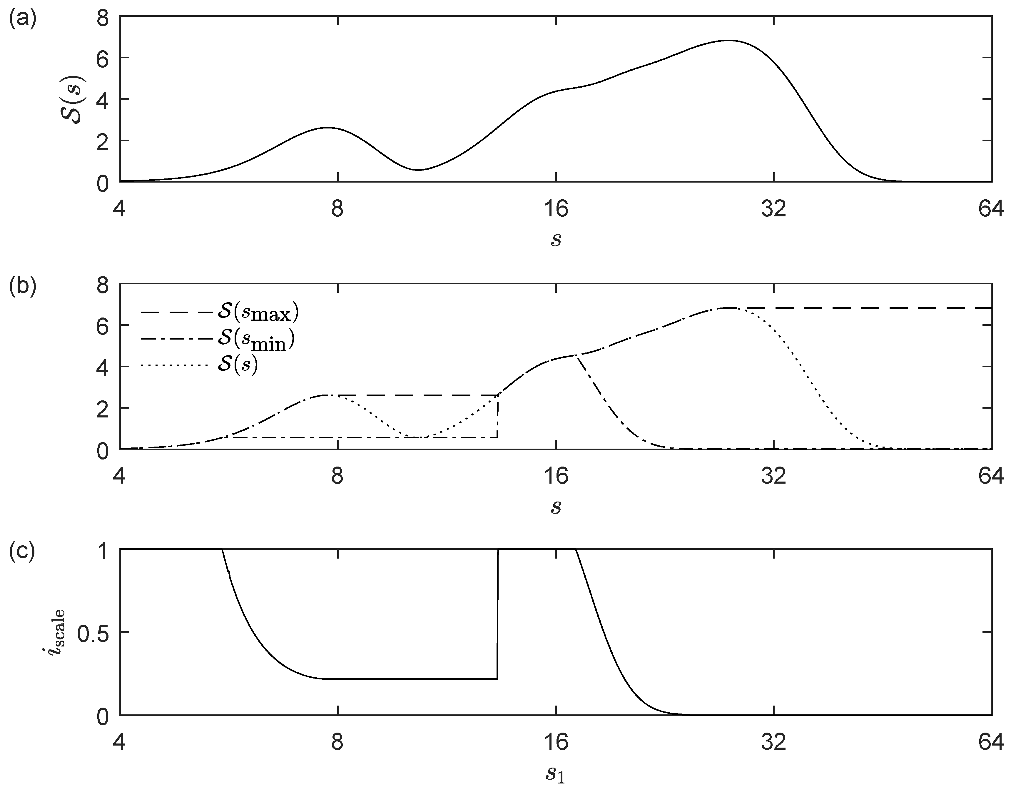
3. The Windowed Scale Index

The scale index given by (9) provides an estimate of the degree of non-periodicity of an entire time series. However, non-stationary signals may pass through different stages in which their behaviour varies considerably and therefore their non-periodicity may not be constant over time. For these cases, we introduce the next definitions.

Definition 3.

The windowed scalogram of a time series f centered at time t with time radius τ is given by

$${\mathcal{WS}}_{\tau }(t,s):={\left({\int }_{t-\tau }^{t+\tau }{\left|Wf\left(u,s\right)\right|}^{2}du\right)}^{1/2}.$$

(10)

The windowed scalogram was previously introduced in [19] and it is just the scalogram given by (3) restricted to a finite time interval $\left[t-\tau ,t+\tau \right]$.

Definition 4.

The windowed scale index of a time series f in the scale interval $[s_0,s_1]$ centered at time t with time radius τ is defined as

$$w{i}_{\mathit{scale},\tau }\left(t\right):=\frac{{\mathcal{WS}}_{\tau }(t,s_{\mathit{min}})}{{\mathcal{WS}}_{\tau }(t,s_{\mathit{max}})},$$

(11)

where, analogously to Definition 2, $s_{\mathit{max}}$ is the smallest scale such that ${\mathcal{WS}}_{\tau }(t,s)\le {\mathcal{WS}}_{\tau }(t,s_{\mathit{max}})$ for all $s\in [s_0,s_1]$, and $s_{\mathit{min}}$ is the smallest scale such that ${\mathcal{WS}}_{\tau }(t,s_{\mathit{min}})\le {\mathcal{WS}}_{\tau }(t,s)$ for all $s\in \left[s_{\mathit{max}},2s_1\right]$.

Although in the computation of the scale index it is recommended the use of normalized inner scalograms in order to avoid border effects, this recommendation is less important in the case of the windowed scale index. This is because for long series and relatively small time radii there would be no border effects in most of the windowed scalograms.

As the original scale index, the windowed scale index is also in the interval $[0,1]$ and it inherits the properties of the scale index that make it a tool for measuring the degree of non-periodicity of a signal around a given time. Precisely, this time dependence makes it a suitable tool for the study of non-stationary signals.

With respect to the choice of the time radius $\tau$, it depends on the nature of the time series f and the objective of the study. In general, it must be big enough so that the windowed scalograms conserve desired (not noisy) information about f, but a too large $\tau$ produces inaccuracy in the location of events for non-stationary time series. Usually, if $\left[a,b\right]$ is the support of f, then $\tau =\left(b-a\right)/20$ is a good choice.

4. Examples and Applications

In this section we illustrate the application of the windowed scale index to different scenarios of non-stationary time series such as chaotic time series, signals affected by non-stationary random noises, and economic and financial time series which present both chaos and noise.

Computations are performed using a self-developed R package [24] called wavScalogram [25], which can be freely downloaded from CRAN.

4.1. The Bonhoeffer-van der Pol Oscillator

As it was done in [5], the applicability of the windowed scale index is illustrated by studying some time series generated by the Bonhoeffer–van der Pol oscillator (BvP), which is given by the following non-autonomous planar system

$$\left.\begin{array}{ccc}\hfill x^{\prime }& =& {\displaystyle x-\frac{x^3}{3}-y+I\left(t\right)}\hfill \\ \hfill y^{\prime }& =& c(x+a-by)\hfill \end{array}\right\},$$

(12)

being $a=0.7$, $b=0.8$, $c=0.1$, and $I\left(t\right)=Acos\left(2\pi t\right)$ an external periodic force. This oscillator is employed for modelling cardiac pulse (see [26]), and hence it is very useful to examine the non-periodicity of a signal without loosing the time location.

Taking the amplitude of the external force A as a parameter, we can construct time series by means of the x coordinate of the solution of (12) with initial conditions $(0,0)$. Specifically, we have created two time series for $A=0.74$ and $A=0.76$, with t from 20 to 400 using a time step of $\mathsf{\Delta }t=0.05$, which are called “series 1” and “series 2”, respectively. Moreover, we have constructed another time series, designated by “series 3”, using $A=0.74$ for $t\in \left[20,400\right]$ and $A=0.76$ for $t\in \left]400,780\right]$. The normalized inner scalograms of these series are displayed in Figure 4, using Daubechies eight–wavelet function and scales running from $0.05$ to $12.8$.

For the computation of the windowed scale indices of these series (see Figure 5), we choose a time radius $\tau =50$ (i.e., 1000 data points), $s_0=0.05$, $s_1=6.4$ and we utilize windowed normalized inner scalograms. This means that we have not taken into account CWTs where the corresponding wavelet overlaps the extremes of the time domain ($\left[20,400\right]$ for series 1 and 2, and $\left[20,780\right]$ for series 3), and the scalograms are normalized as it is shown in Definition 1. As a curiosity, the global scale index of series 3 is approximately $0.4494$, which is greater than the scale index of series 1 ($0.0768$ approx.) and series 2 ($0.4116$ approx.). Figure 6 depicts the different stages for obtaining the windowed scale indices of series 3 for a wide set of values of $s_1$, ranging from $0.4$ to $6.4$. In this way, we can see the importance of the choice of $s_1$. Note that Figure 5 only plots the windowed scale indices for $s_1=6.4$.

As can be seen in Figure 5, the windowed scale index clearly shows the evolution of the scale index over time, which is an important improvement, and is more appropriate for studying non-stationary signals than the global scale index. Specifically, Figure 5c illustrates the usefulness of the windowed scale index in detecting the jump in the non-periodicity due to the change in the amplitude of the external force, while the global scale index described in [5] only gives an overall value for the whole time span.

4.2. A Signal with Increasing Noise

The windowed scale index is not only useful to study chaotic signals, as the one seen in the above example, but it also enables analysing other non-stationary signals such as those affected by non-stationary random noises. For example, we may consider a signal of the form

$$f\left(t\right)=sin\left(2\pi t\right)+{ϵ}_t,{ϵ}_t\sim \mathcal{N}\left(\mu =0,{\sigma }^2=0.1t\right),$$

(13)

which corresponds to a 1-periodic signal plus a Gaussian noise term ${ϵ}_t$ with increasing variance. Figure 7 depicts the average of the windowed scale indices of 1000 series of the form described by (13) taking $s_0=0.02$ and different $s_1$ values, using Morlet wavelets and time radius $\tau =5$. Since there is a 1-periodic term, $s_1$ must be greater or equal than 1 in order to detect this periodicity. However, choosing a too large $s_1$ has drawbacks: the larger $s_1$ is, the lower the noise sensitivity will be, as shown in Figure 7. This figure also illustrates how the windowed scale index succeeds in describing the nature of signals with non-stationary noises, as it gets larger over time as the noise of the signal increases, according to what would be expected.

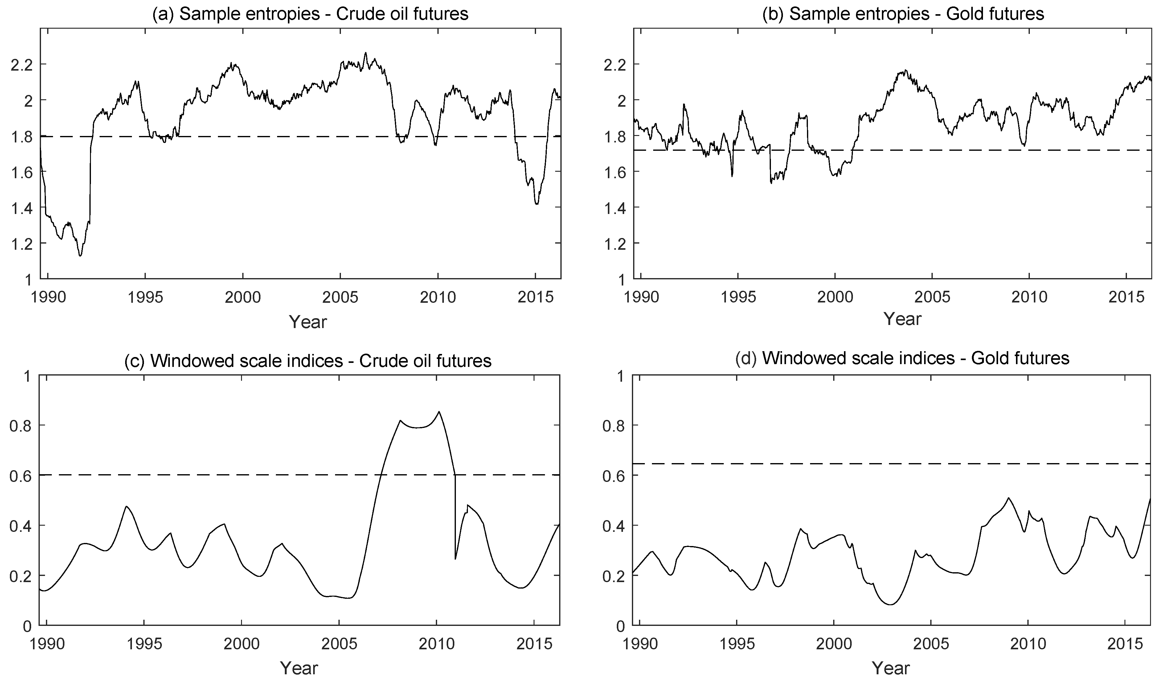
4.3. An Economic Application: Crude Oil and Gold Prices

An interesting application of the windowed scale index in the field of economics consists of quantifying the degree of non-periodicity of the price of two major commodities such as crude oil and gold at different points in time and for certain ranges of scale. This analysis allows one to determine to what extent these time series have a periodical or repetitive behaviour.

Crude oil and gold are the most actively traded mineral commodities in the world and play a critical role in human civilization. As mentioned by [27], oil is by far the most strategic commodity and the most sizable source of energy for the modern economy as it constitutes a vital input in the production process of many goods and services. The importance of crude oil is so great that changes in oil price affect strongly global economic growth, inflation and asset values. Meanwhile, gold is the leader in precious metal markets and is demanded for jewelry purposes and for many other industries such as dental, electronics and chemicals. Furthermore, gold has had a unique historic function as a means of exchange and a store of value for millennia and, more recently, as an alternative investment that hedges against inflation, a falling U.S. dollar or other forms of uncertainty. Due to its singular nature, gold is widely considered to be an effective safe haven asset against losses in financial markets, especially in times of financial and economic instability [28,29,30].

The dataset used in this application consists of daily closing prices of futures contracts for gold and crude oil. Specifically, for oil the prices from nearby contracts of crude oil futures traded on the New York Mercantile Exchange (NYMEX) are utilized. For gold, the nearby contract prices of gold futures traded on the COMEX division of the NYMEX, which is the most liquid gold contract in the world, are employed. Changes in prices of oil and gold futures contracts are used in order to better capture the possible repetitive or periodical nature of these two series. The sample period spans from 24 June 1988 until 20 June 2017, with a total of 7564 daily observations. All data are collected from Thomson Reuters DataStream.

Figure 8 displays the windowed scalograms and windowed scale indices of changes in the price of crude oil and gold futures contracts. The windowed scalograms use a time radius $\tau =300$ days and the windowed scale indices are calculated from these windowed scalograms taking $s_0=8$ days and a wide range of scales $s_1$, from 32 to 512 days. We have not used inner scalograms in this case. Therefore, the corresponding cones of influence outside which there are border effects have been plotted.

It is shown that the windowed scale indices for oil futures contracts take very high values in the time period between 2007 and 2010 for scale intervals with $s_1$ between 150 and 300 days, which are representative of the medium term. This finding may be closely related to an important shift in the behaviour of oil price from 2007. In particular, as can be seen in the windowed scalograms for crude oil futures contracts in plot (a) of Figure 8, the scales between 256 days (approximately one year) and 512 days (two years) become the scales that contribute most to the energy of the oil price series during the period 2007–2010, and by taking $s_1$ less than 300, these important scales are not taken into account. Hence, these high values of the windowed scale indices for oil futures can be interpreted as an evident symptom of unpredictability (see Section 4.4) in oil price at the medium term during the period around the financial crisis that started in mid-2007 in the U.S. subprime mortgage market and spread throughout the world from September 2008 following the collapse of the U.S. investment bank Lehman Brothers. During this period, crude oil price experienced drastic rises and falls mostly driven by positive and negative shifts in global aggregate demand. For example, as noted by [31], the rapid increase in the spot price per barrel of West Texas Intermediate (WTI) crude oil from USD 58 in January 2007 to USD 140 in June 2008 may be associated with a strong global economic activity. In turn, the decline in oil price to USD 41.68 in January 2009 may be attributed to the global financial crisis and the subsequent great recession. However, the WTI oil price rebounded to USD 133.93 in April 2011, even though global economic activity remained moderate. Therefore, the abnormally volatile development of crude oil price over the last years may have largely contributed to the high degree of unpredictability of oil price at the medium term around the recent global financial crisis, which is captured by the windowed scale indices.

In contrast, the windowed scale indices for gold futures contracts do not take generally high values despite the fact that during the global financial crisis period, there were also significant changes in the energies contributed by most of the scales, as depicted in plot (c) of Figure 8. This result indicates a more predictable behaviour of the price of gold for all time scales over the last few decades in comparison with oil prices. One possible explanation for this finding is related to the fact that gold price has followed a secular upward trend, which has been only interrupted sporadically and for very short periods of time. In this regard, unlike conventional financial assets such as stocks or bonds, gold price tends to increase notably even during periods of increased economic uncertainty, such as the global financial crisis that started in 2008 or the COVID-19 pandemic since March 2020. Therefore, the safe haven nature of gold, particularly in times of market turbulence, seem to play a key role in its more predictable (periodic) behaviour compared to that of crude oil over the past few decades.

Apart from the case of these two major commodities, there may be many other potentially meaningful applications of the windowed scale index in economics and finance. For example, it could be very interesting to assess the degree of unpredictability of the cryptocurrency market, paying special attention to the main cryptocurrencies, including bitcoin, ripple and ethereum. The analysis of the regularity of price fluctuations in currency markets appears as another promising application of the new wavelet-based tool in order to identify the particular exchange rates which exhibit a more irregular behaviour. In the same vein, the windowed scale index could be also used to measure the level of unpredictability or randomness of some conventional financial markets such as stock or bond markets. Given the huge total market capitalization of these traditional markets, this knowledge will have important practical implications for investors and policy makers.

4.4. Non-Periodicity and Unpredictability

So far, we have showed how the windowed scale index can be used to assess the degree of non-periodicity of a time series over time and thus it has been proven useful for determining shifts in the periodicity regime. Since periodicity and predictability represent closely related concepts, it seems reasonable to compare the windowed scale index with a standard measure of the level of unpredictability of a time series.

The sample entropy (SampEn) [2] is a measure of the signal’s complexity and ultimately of its unpredictability, in the sense that the higher the SampEn is, the more unpredictable the signal will be. In essence, the SampEn is a modification of the approximate entropy (AppEn) [1], which was designed to measure the unpredictability of time series, but it overcomes some of the limitations of the AppEn, such as the signal length dependence. Both measures are based on the Kolmogorov-Sinai statistic [32] and have been mainly used in the analysis of biomedical data (e.g., EEG signals). Similarly, the scale index (global or windowed) may also be seen as a measure of a time series unpredictability in so far as the degree of non-periodicity intuitively gives us an insight into how the future values of a signal may be predicted from the past ones.

In order to compare the SampEn with the windowed scale index, the sample entropies are computed on a rolling window of the same radius as the one employed for the windowed scale indices estimation. The computations are performed using the R statistical software and the SampEn functions provided by the package pracma [33]. For the artificial signals generated by the Bonhoeffer-van der Pol chaotic dynamical system, Figure 9 depicts the sample entropies for a rolling window of radius $\tau =50$ observations and the global SampEn calculated for the whole signal. Although the overall value of the SampEn is slightly higher for time series 2, which corresponds to a more chaotic signal than time series 1, the difference is so small that it can be considered negligible. By contrast, when comparing Figure 9 with Figure 5, it can be seen that the windowed scale index is able to clearly distinguish between different degrees of chaos or non-periodicities.

Likewise, the sample entropies are estimated for the crude oil and gold futures contracts in Figure 10, plots (a) and (b), using a rolling window of radius $\tau =300$ days. The global SampEn for the oil futures contracts series yields overall higher values than for the gold futures contracts (dashed lines), but the differences are again very small. On the other hand, the sample entropies estimated on a rolling window (solid line) take, for certain time intervals, larger values for the crude oil futures than for the gold futures contracts, and vice versa. In order to compare with the windowed scale index, in Figure 10, plots (c) and (d), we also show the sections at $s_1=256$ days (a scale representative of the medium term) of the windowed scale indices plots of Figure 8, in which a time radius of $\tau =300$ days was also employed. Moreover, the corresponding global scale index is represented by a dashed line. It can be seen that the windowed scale indices of crude oil futures contracts increase considerably during the global financial crisis, unlike what happens with the gold futures contracts. Besides, the global scale index of the gold futures contracts is slightly greater than the global scale index of the crude oil futures contracts, showing that in this case, the windowed scale index provides more reliable and detailed information than the global scale index.

Therefore, according to this example, the windowed scale index has demonstrated to be a valuable tool for the analysis of the level of unpredictability since it is able to detect changes in the time series that go unnoticed for other tools such as the SampEn. In essence, the windowed scale index presents two major advantages over the SampEn and the AppEn. The first one is about the interpretability. Specifically, the windowed scale index takes values between 0 and 1 and this boundedness allows us to clearly state how non-periodic a time series is. Meanwhile, the SampEn and AppEn are not bounded, so it is harder to say whether a given entropy value is high or low and, consequently, whether a given time series is highly unpredictable or not. A second advantage of the windowed scale index over the entropy parameters is its sensitivity. In particular, the windowed scale index presents a higher sensitivity to distinguish between different levels of non-periodicity. For instance, while the windowed scale index is able to clearly identify that time series 1 in the BvP oscillator example is much less non-periodic than time series 2, the SampEn values are almost identical.

5. Conclusions

The scale index proposed by [5] has proved to be a helpful wavelet tool to assess the degree of non-periodicity of a time series. This usefulness is based on the result according to which the wavelet transform of a periodic time series vanishes when the scale is twice the period. From a theoretical point of view, it is very interesting to study whether the converse is true or not. In this paper, it is shown that, at least for the Haar wavelet, the vanishing of the wavelet transform at a certain scale (for all times) guarantees the periodic character of the time series.

The windowed scale index introduced in this paper has its origin in the scale index and is particularly adequate to measure the degree of non-periodicity of non-stationary signals, whose characteristics may vary over time. Moreover, the use of the windowed scale index as a measure of unpredictability has advantages in terms of interpretability and sensitivity over some standard unpredictability measures such as the SampEn or the AppEn. Furthermore, in order to facilitate the use of this and other related wavelet-based tools, we have developed an R package named wavScalogram [25], which provides researchers unfamiliar with wavelet analysis a user-friendly framework for identifying the non-periodicity characteristics of time series.

This paper also includes an economic application of this novel wavelet tool in which the level of unpredictability of two crucial commodities for the world economy, such as crude oil and gold, is quantified. The results reveal that oil futures contracts exhibit a higher degree of non-periodicity than gold futures contracts, particularly in the medium term during the period around the global financial crisis. One possible explanation for the greater unpredictability of oil is related to the abrupt fluctuations in crude oil prices caused by positive and negative changes in global aggregate demand since 2007. However, the more predictable behaviour of the price of gold regardless of the specific time interval and scale can be attributed to its secular upward trend, which can be seen as a consequence of the traditional consideration of gold as a safe haven asset, especially during episodes of financial turmoil.

Given the steady growth in the number of research articles and fields of knowledge that have applied the scale index over the last few years, we strongly believe that the windowed scale index has a great potential to be widely used in future work. On the one hand, this tool can be particularly useful in numerous scientific disciplines, such as physics, seismology, climatology, medicine or engineering, to shed more light on the non-periodicity features of non-stationary signals or time series. For example, the windowed scale index can play a critical role in the field of pseudo random number generators (PRNG), not only to assess the degree of non-periodicity of the PRNG, but also to check for stationarity, which could be a relevant indicator of the goodness of the algorithm. On the other hand, the windowed scale index also has a high applicability in the area of economics and finance. For instance, the proper identification of the level of unpredictability of several major financial markets, such as the exchange rate, stock or cryptocurrency markets, can have valuable economic implications for investors, portfolio managers and policy makers. In addition, the wavelet tools proposed in this paper can be of interest for anyone working with long enough time series, such as those typically handled by national and international statistical institutions.

References

1. Pincus, S.M.; Gladstone, I.M.; Ehrenkranz, R.A. A regularity statistic for medical data analysis. J. Clin. Monit. 1991, 7, 335–345. [Google Scholar] [CrossRef] [PubMed]
2. Richman, J.S.; Moorman, J.R. Physiological time-series analysis using approximate entropy and sample entropy. Am. J. Physiol.-Heart Circ. Physiol. 2000, 278, H2039–H2049. [Google Scholar] [CrossRef] [PubMed] [Green Version]
3. Bandt, C.; Pompe, B. Permutation Entropy: A Natural Complexity Measure for Time Series. Phys. Rev. Lett. 2002, 88, 174102. [Google Scholar] [CrossRef] [PubMed]
4. Henry, M.; Judge, G. Permutation Entropy and Information Recovery in Nonlinear Dynamic Economic Time Series. Econometrics 2019, 7, 10. [Google Scholar] [CrossRef] [Green Version]
5. Benítez, R.; Bolós, V.J.; Ramírez, M.E. A wavelet-based tool for studying non-periodicity. Comput. Math. Appl. 2010, 60, 634–641. [Google Scholar] [CrossRef] [Green Version]
6. Hesham, M. Wavelet-scalogram based study of non-periodicity in speech signals as a complementary measure of chaotic content. Int. J. Speech Technol. 2013, 16, 353–361. [Google Scholar] [CrossRef]
7. Akhshani, A.; Akhavan, A.; Mobaraki, A.; Lim, S.C.; Hassan, Z. Pseudo random number generator based on quantum chaotic map. Commun. Nonlinear Sci. Numer. Simul. 2014, 19, 101–111. [Google Scholar] [CrossRef]
8. Avaroğlu, E.; Tuncer, T.; Özer, A.B.; Ergen, B.; Türk, M. A novel chaos-based post-processing for TRNG. Nonlinear Dyn. 2015, 81, 189–199. [Google Scholar] [CrossRef]
9. Yang, Y.G.; Xu, P.; Yang, R.; Zhou, Y.H.; Shi, W.M. Quantum Hash function and its application to privacy amplification in quantum key distribution, pseudo-random number generation and image encryption. Sci. Rep. 2016, 6, srep19788. [Google Scholar] [CrossRef] [Green Version]
10. Yang, Y.G.; Zhao, Q.Q. Novel pseudo-random number generator based on quantum random walks. Sci. Rep. 2016, 6, srep20362. [Google Scholar] [CrossRef] [Green Version]
11. Tuncer, T. The implementation of chaos-based PUF designs in field programmable gate array. Nonlinear Dyn. 2016, 86, 975–986. [Google Scholar] [CrossRef]
12. Murillo-Escobar, M.A.; Cruz-Hernández, C.; Cardoza-Avendaño, L.; Méndez-Ramírez, R. A novel pseudorandom number generator based on pseudorandomly enhanced logistic map. Nonlinear Dyn. 2017, 87, 407–425. [Google Scholar] [CrossRef]
13. Yang, Y.G.; Pan, Q.X.; Sun, S.J.; Xu, P. Novel Image Encryption based on Quantum Walks. Sci. Rep. 2015, 5, srep07784. [Google Scholar] [CrossRef] [PubMed] [Green Version]
14. Fan, Q.; Wang, Y.; Zhu, L. Complexity analysis of spatial–temporal precipitation system by PCA and SDLE. Appl. Math. Model. 2013, 37, 4059–4066. [Google Scholar] [CrossRef]
15. Behnia, S.; Ziaei, J.; Ghiassi, M.; Yahyavi, M. Comprehensive Chaotic Description of Heartbeat Dynamics Using Scale Index and Lyapunov Exponent. In Proceedings of the 6th Chaotic Modeling and Simulation International Conference, Istanbul, Turkey, 11–14 June 2013; Volume 500, pp. 1–5. [Google Scholar]
16. Felix, J.L.P.; Balthazar, J.M.; Tusset, A.M.; Piccirillo, V.; Bueno, A.M.; Brasil, R.M.L.R.F. On Optimal Control of a Nonlinear Robotic Mechanism Using the Saturation Phenomenon. In Structural Nonlinear Dynamics and Diagnosis; Springer Proceedings in Physics; Springer: Cham, Switzerland, 2015; pp. 145–165. [Google Scholar] [CrossRef]
17. Piccirillo, V.; Balthazar, J.M.; Tusset, A.M.; Bernardini, D.; Rega, G. Characterizing the nonlinear behavior of a pseudoelastic oscillator via the wavelet transform. Proc. Inst. Mech. Eng. Part C J. Mech. Eng. Sci. 2016, 230, 120–132. [Google Scholar] [CrossRef]
18. Jiménez, D.S.; Stahl, P.; Terminel, O. Mechanical fault identification using Wavelet Transform and Labview. Nova Sci. 2015, 7, 162–177. [Google Scholar] [CrossRef] [Green Version]
19. Bolós, V.J.; Benítez, R.; Ferrer, R.; Jammazi, R. The windowed scalogram difference: A novel wavelet tool for comparing time series. Appl. Math. Comput. 2017, 312, 49–65. [Google Scholar] [CrossRef]
20. Mallat, S. A Wavelet Tour of Signal Processing: The Sparse Way; Academic Press: Cambridge, MA, USA, 2008. [Google Scholar]
21. Torrence, C.; Compo, G.P. A Practical Guide to Wavelet Analysis. Bull. Am. Meteorol. Soc. 1998, 79, 61–78. [Google Scholar] [CrossRef] [Green Version]
22. Liu, Y.; San Liang, X.; Weisberg, R.H. Rectification of the Bias in the Wavelet Power Spectrum. J. Atmos. Ocean. Technol. 2007, 24, 2093–2102. [Google Scholar] [CrossRef]
23. Torrence, C.; Webster, P.J. Interdecadal Changes in the ENSO–Monsoon System. J. Clim. 1999, 12, 2679–2690. [Google Scholar] [CrossRef] [Green Version]
24. R Core Team. R: A Language and Environment for Statistical Computing; R Foundation for Statistical Computing: Vienna, Austria, 2017. [Google Scholar]
25. Bolós, V.J.; Benítez, R. wavScalogram: Wavelet Scalogram Tools for Time Series Analysis; R Package Version 1.0.0; 2019; Available online: https://CRAN.R-project.org/package=wavScalogram (accessed on 1 May 2020).
26. Scott, A. Neurophysics; Wiley: New York, NY, USA, 1977. [Google Scholar]
27. Aguilera, R.F.; Radetzki, M. The synchronized and exceptional price performance of oil and gold: Explanations and prospects. Resour. Policy 2017, 54, 81–87. [Google Scholar] [CrossRef]
28. Baur, D.G.; Lucey, B.M. Is gold a hedge or a safe haven? An analysis of stocks, bonds and gold. Financ. Rev. 2010, 45, 217–229. [Google Scholar] [CrossRef]
29. Baur, D.G.; McDermott, T.K. Is gold a safe haven? International evidence. J. Bank. Financ. 2010, 24, 1886–1898. [Google Scholar] [CrossRef]
30. Ciner, C.; Gurdgiev, C.; Lucey, B.M. Hedges and safe havens: An examination of stocks, bonds, gold, oil and exchange rates. Int. Rev. Financ. Anal. 2013, 29, 202–211. [Google Scholar] [CrossRef]
31. Ratti, R.A.; Vespignani, J.L. Why are crude oil prices high when global activity is weak? Econ. Lett. 2013, 21, 133–136. [Google Scholar] [CrossRef] [Green Version]
32. Sinai, Y.G. On the notion of entropy for a dynamic system. Dokl. Russ. Acad. Sci. 1959, 124, 768–771. [Google Scholar]
33. Borchers, H.W. pracma: Practical Numerical Math Functions; R Package Version 2.2.9; 2019; Available online: https://CRAN.R-project.org/package=pracma (accessed on 1 May 2020).
Figure 1. (a) Scalogram (using Morlet wavelet) of the signal i = 1 6 sin 2 π T i t with t 0 , 1000 and T i = 8 , 16 , 20 , 24 , 28 , 32 for i = 1 , , 6 respectively, i.e., a combination of several signals of periods T i . (b) The same scalogram as above (dotted), jointly with S s max (dashed) and S s min (dash-dotted) taking s 0 = 4 and s 1 = s . (c) The corresponding scale index (i.e., S s min / S s max ) taking s 0 = 4 and s 1 varying from 4 to 64.
Mathematics 08 00844 g001
Figure 2. (a) Scalogram (using Morlet wavelet) of the signal sin 2 π 8 t + sin 2 π 16 t with t 0 , 1000 , i.e., a combination of two signals of period 8 and 16 respectively with the same amplitude. There are two local maxima at the scales corresponding with the periods 8 and 16 respectively, but the scalogram takes different maximum values at these scales. (b) The same scalogram multiplied by the factor 1 s . Now, the scalogram takes the same maximum values, showing that both scales contribute with the same “energy”.
Mathematics 08 00844 g002
Figure 3. (a) Mean of the scalograms of 100 random uniform series in 1 , 1 of 10,000 data points, using Morlet wavelet. It can be seen that it is more or less constant and so, the corresponding scale index would be close to 1 for any s 1 . (b) Mean of the 100 scalograms of the same random uniform series but multiplied by the factor 1 s . It tends to zero for large scales and so, the scale index computed from this modified scalogram would also tend to zero as we increase s 1 .
Mathematics 08 00844 g003
Figure 4. Normalized inner scalograms of series 1, 2 and 3 (see (a), (b) and (c) respectively), using Daubechies eight–wavelet. The scale runs from 0.05 to 12.8 .
Mathematics 08 00844 g004
Figure 5. Windowed scale indices of series 1, 2 and 3 (see (a), (b) and (c) respectively), centered at different times with time radius τ = 50 . The scale parameters run from s 0 = 0.05 to s 1 = 6.4 and we use Daubechies eight–wavelet function. The corresponding global scale index is represented with a dashed line.
Mathematics 08 00844 g005
Figure 6. Different stages for obtaining the windowed scale indices of series 3. (a) Moduli of the CWT. (b) Windowed scalograms centered at different times with time radius τ = 50 . (c) Windowed scale indices centered at different times with time radius τ = 50 , taking s 0 = 0.05 and different values of s 1 from 0.4 to 6.4 . The cone of influence outside which there are border effects is also represented with a black line in all plots.
Mathematics 08 00844 g006
Figure 7. Average of the windowed scale indices of 1000 series of the form (13) taking s 0 = 0.02 and different values for s 1 , using Morlet wavelets and time radius τ = 5 . The cone of influence outside which there are border effects is represented with a black line (a) and dots (b).
Mathematics 08 00844 g007
Figure 8. (a) Windowed scalograms and (b) windowed scale indices of crude oil futures contracts price returns. (c) Windowed scalograms and (d) windowed scale indices of gold futures contracts price returns. The windowed scalograms are centered at different times with time radius τ = 300 days. The windowed scale indices are centered at different times with time radius τ = 300 days, taking s 0 = 8 days and different values of s 1 from 32 to 512 days. The cone of influence outside which there are border effects is also represented with a black line in all plots.
Mathematics 08 00844 g008
Figure 9. Sample entropies of series 1, 2 and 3 (see (a), (b) and (c) respectively) considering subseries centered at different times with time radius τ = 50 . The corresponding global SampEn is represented with a dashed line.
Mathematics 08 00844 g009
Figure 10. Sample entropies and windowed scale indices of crude oil and gold futures contracts price returns. For the sample entropies (see (a,b)), we have considered subseries centered at different times with time radius τ = 300 days. With respect to the windowed scale indices (see (c,d)), they are centered at different times with time radius τ = 300 days, taking s 0 = 8 days and s 1 = 256 days. The corresponding global SampEn and scale index are represented with dashed lines.
Mathematics 08 00844 g010