Using an Adaptive Fuzzy Neural Network Based on a Multi-Strategy-Based Artificial Bee Colony for Mobile Robot Control

Abstract

This study proposes an adaptive fuzzy neural network (AFNN) based on a multi-strategy artificial bee colony (MSABC) algorithm for achieving an actual mobile robot navigation control. During the navigation control process, the AFNN inputs are the distance between the ultrasonic sensors and the angle between the mobile robot and the target, and the AFNN outputs are the robot’s left- and right-wheel speeds. A fitness function in reinforcement learning is defined to evaluate the navigation control performance of AFNN. The proposed MSABC algorithm improves the poor exploitation disadvantage in the traditional artificial bee colony (ABC) and adopts the mutation strategies of a differential evolution to balance exploration and exploitation. To escape in special environments, a manual wall-following fuzzy logic controller (WF-FLC) is designed. The experimental results show that the proposed MSABC method has improved the performance of average fitness, navigation time, and travel distance by 79.75%, 33.03%, and 10.74%, respectively, compared with the traditional ABC method. To prove the feasibility of the proposed controller, experiments were carried out on the actual PIONEER 3-DX mobile robot, and the proposed navigation control method was successfully completed.

1. Introduction

The navigation control of mobile robots is a popular research topic in the robot study area. Navigation is an easy task for animals and humans as they have the ability to think. However, it is difficult for robots because they lack this ability. The robot navigation method has been classified into the hybrid behavior [1,2] and the behavior-based methods [3,4,5,6,7,8]. In the hybrid behavior, Seraji and Howard [1] used a distance sensor and a camera for detecting the environment around a robot. The robot navigation strategy has been designed using three independent behaviors, regional traverse–terrain, local avoid–obstacle, and global seek–goal. Finally, the center of gravity method was used by three consecutive defuzzifier steer angles and speeds of a robot navigating in an unknown environment. Foudil et al. [2] divided navigation control into two fuzzy controllers, obstacle avoidance and goal seeking, which were used to design the steer angle of obstacle avoidance and the goal seeking rule table. Thereafter, the outputs of the two fuzzy controllers, which controlled the steer angle of the mobile robot, were combined. In particular, the fuzzy controller for the obstacle avoidance task was designed using the distance sensor. By contrast, the mobile robot used the hierarchy fuzzy controller for the obstacle avoidance task, assuming that the mobile robot can accurately control the navigation. In the behavior-based method, Pratihar et al. [3] addressed the problem of mobile robot navigation in any environment. They used a fuzzy controller to design the steer angle of the mobile robot and a genetic algorithm (GA) was applied to determine the optimal antecedent parameter that determines the best fuzzy controller implication in a mobile robot automatic navigation task. Boubertakh et al. [4] proposed an improved fuzzy Q-learning (IFQ) algorithm and used IFQ reinforcement-learned navigation in an unknown environment. Juang and Chang [5] proposed a particle swarm optimization (PSO) group-based application fuzzy controller. A new reinforcement-learning wall-following fuzzy controller is proposed and adapts to any environment. Last, according to distance information of sensors that switch wall-following control and goal seeking control, Yang et al. [6] proposed a new switch strategy that determines obstacle avoidance and goal seeking in an unknown environment, in accordance with the Q-learning in which the mobile robot learns to determine obstacle avoidance and goal seeking. Moreover, they used a neural network to determine the current environment through weight calculation of the left- and right-wheel speeds of the mobile robot. Learning of the neural network is an application genetic algorithm that coding for the optimal best weight makes the neural network slow down in error. Finally, the new switch strategy is combined with the existing one for obtaining mobile robot navigation. Nakhaeinia and Karasfi [7] used a fuzzy controller in which the obstacle position controlled the mobile robot speed and a steer angle. A laser is used as a distance sensor for scanning an unknown environment. When a mobile robot is in a concave environment, it produces a visual target in the neighborhood environment. The mobile robot is given up the path of actual target change to go to the path of the visual target. When the mobile robot reaches the visual target, repeating the planned path of the actual target, which escapes the local trap, the navigation task is completed. Mohanty and Parhi [8] used a neural fuzzy network controller that solves the mobile robot navigation problem. A distance sensor is applied to acquire information about the angle between the goal and the mobile robot. They also used the backpropagation algorithm to determine the best neural fuzzy controller. Finally, the experimental result indicated that a neural fuzzy controller can perform the navigation problem and address the shortcoming of parameter definition in a traditional fuzzy controller.

The definition of a neural fuzzy controller parameter is a popular research topic. Recently, evolutionary algorithms (EAs) [9,10] for creating optimal controller parameters have been extensively researched. EA is an inspirational algorithm in which a random search is usually applied to a complex space or multiple modules (actual function application is unknown). In addition, the EA may fall into a suboptimal solution. Individual EAs mainly imitate biological behavior and populations, which make EA development an important field of study. Most well-known algorithms have been widely applied as GA [11], PSO [12], and differential evolution (DE) [13]. These algorithms have been successful used in many optimal parameter problems. GA exhibits the best ability for global solution space. However, it can easily fall into the local minimum and its search solution takes considerable time [14]. The PSO algorithm, proposed by Kennedy and Eberhart, imitates bird and fish behaviors for finding food. This algorithm applies the concept of cluster movement for determining the front best solution in the search space. The algorithm can easily be applied in the optimization technology because it has a strong search ability and, therefore, has been applied to many actual fields [15,16]. The DE algorithm is a parallel and direct search technology. It has a strong search ability and convergence ability for the application of optimal real numbers [17,18,19], but still suffers from accuracy and stability problems [20]. Yang [21] proposed the virtual bee algorithm to optimal functions of two dimensions, which is produced after the star movement in search space interact with each other while the bee finds some food. The solution of this problem lies in defining each bee’s interaction strength. Pham et al. [22] proposed another bee algorithm that uses several control parameters. To address the function of multiple variables and multiple modules, Karaboga and Basturk [23] proposed an artificial bee colony algorithm (ABC). They use ABC compare the other algorithm test some problems [24,25,26]. They expanded the application of the ABC algorithm for solving the traveling salesman problem [27], discovery of conserved regions in DNA sequences [28], and training ANFIS [29].

In this study, an adaptive fuzzy neural network (AFNN) based on a multi-strategy artificial bee colony (MSABC) algorithm is proposed for achieving an actual mobile robot navigation control and escape special environment behavior to avoid special obstacles. The proposed AFNN is a four-layer structure. Nodes in layer one represent input linguistic variables. Nodes in layer two act as membership functions, which express the input fuzzy linguistic variables. Gaussian membership functions are used in this layer. Nodes in layer three are equal to the number of fuzzy sets that correspond to each external input linguistic variable. The node in layer four is called the output node. During the navigation control process, the distance between the ultrasonic sensor and the obstacle and the angle between the mobile robot and the target are used as inputs of the AFNN, and the robot’s left- and right-wheel speeds are used as outputs of the AFNN. In the AFNN, the definition of fuzzy membership function in layer two is used to calculate the membership degree of the distance and the angle during the navigation control process. A fitness function is defined to evaluate the AFNN performance in the navigation control. The fitness function includes the following three control factors: navigation time, distance between the start and the target, and distance between the mobile robot and target travel. The traditional ABC algorithm simulates the intelligent foraging behavior of honey-bee swarms, which are good at exploration but poor at exploitation. The proposed MSABC algorithm adopts the mutation strategies of a differential evolution to balance exploration and exploitation.

The remainder of the paper is organized as follows. Section 2 introduces the structure of a Pioneer 3-DX mobile robot. Details on AFNN and its related MSABC learning algorithm are described in Section 3. Section 4 presents navigation control of a mobile robot. The experimental results of mobile robot navigation control are illustrated in Section 5. Section 6 offers conclusions for this study.

2. The Structure of Pioneer 3-DX Mobile Robot

In this section, a Pioneer 3-DX mobile robot is introduced and shown in Figure 1a. This robot is heavy, has a long movement time, and can be widely applied to problems such as laser mapping, navigation, and stereo vision systems. The robot body has dimensions of 45 × 38 × 25 cm³. This robot is equipped with eight sonar sensors, which detect the surrounding unknown environment, as shown in Figure 1b. The sonar sensors conduct measurements in between approximately 0.15 and 4.75 m. In addition, the robot is equipped with two wheels and one caster, with a maximum speed of 1.2 m/s, as well as a compass, which provides current direction.

In this study, the original sensor values have a lower detection range of approximately 0.2–3 m in the simulation and experiments, as a larger range is unnecessary for a training environment. The eight ultrasonic sensors (S₀, S₁, …, S₇) were allocated into three signs: Left, Front, and Right. Left is the distance between the obstacle and left sensor (i.e., S₀, and S₁) of the robot, Front is the distance between the obstacle and the front sensor (i.e., S₂, S₃, S₄ and S₅) of the robot, and Right is the distance between the obstacle and right sensor (i.e., S₆ and S₇) of the robot.

3. The Proposed Controller and Its Related Learning Algorithm

In this section, an adaptive fuzzy neural network (AFNN) is proposed and its related multi-strategy artificial bee colony (MSABC) learning algorithm is also presented.

3.1. An Adaptive Fuzzy Neural Network (AFNN)

Figure 2 presents the structure of the AFNN. Nodes in layer one are input nodes, which represent input linguistic variables. Nodes in layer two are called membership function nodes and act as membership functions, which express the input fuzzy linguistic variables. Nodes in this layer are used to determine Gaussian membership values. That is, the degrees of fuzzy membership of the Left, Front, and Right in Figure 1 are calculated through layer two, where each input linguistic variable is mapped to a value between 0 and 1. Each node in layer three is called a compensatory fuzzy rule node. Nodes in layer three are equal to the number of fuzzy sets that correspond to each external input linguistic variable. The node in layer four is called the output node. The j_th rule in AFNN can be expressed as

$$\mathrm{Rule}\begin{array}{c}-\end{array}j:\begin{array}{c}\end{array}\mathrm{IF}\begin{array}{c}[\end{array}{x}_1\begin{array}{c}\end{array}\mathrm{is}\begin{array}{c}\end{array}{A}_{1j}\begin{array}{c}\end{array}\mathrm{and}\begin{array}{c}\end{array}{x}_2\begin{array}{c}\end{array}\mathrm{is}\begin{array}{c}\end{array}{A}_{2j}\dots \mathrm{and}\begin{array}{c}\end{array}{\begin{array}{c}x\end{array}}_i\begin{array}{c}\end{array}\mathrm{is}\begin{array}{c}\end{array}{A}_{ij}\dots \begin{array}{c}\mathrm{and}\begin{array}{c}\end{array}\end{array}{\begin{array}{c}x\end{array}}_N\begin{array}{c}\end{array}\mathrm{is}\begin{array}{c}\end{array}{A}_{Nj}{]}^{1-{\gamma }_j+\frac{{\gamma }_j}{N}}$$

$${\mathrm{THEN}\hat{\mathrm{y}}\mathrm{is}\mathrm{w}}_j$$

where x_i is the input linguistic variable, $\hat{\mathrm{y}}$ is the output variable, A_ij is the linguistic term of the precondition part, ${\gamma }_j\in [0,1]$ is the compensatory factor, w_j is the weight of the consequent part, and N is the number of input linguistic variables. Each layer is detailed below:

Layer one (Input Node): This layer of each node is the input term node and each node corresponds to each linguistic term. In this node, the information is directly input to the next layer.

$$u_i^{(1)}=x_i$$

(1)

Layer two (Membership Function Node): This layer of each node is the input linguistic node. Layer two performs the fuzzification operation, which calculates the membership value corresponding to the degree to which an input value belongs to a fuzzy set in layer two. In this study, the Gaussian membership function is used in layer two.

$$u_{ij}^{(2)}=\exp \left(\frac{-{[u_i^{(1)}-m_{ij}]}^2}{{\sigma }_{ij}^2}\right)$$

(2)

where m_ij and σ_ij represent the mean and standard deviation of the Gaussian membership function, respectively, of the j_th term of the i_th input linguistic variable x_i.

Layer three (Compensatory Rule Node): This layer denotes a compensatory fuzzy rule node, where each node represents each fuzzy rule. This layer performs the fuzzy rule influence operation. By contrast, the node computes the fuzzy product operation. Thereafter, it is applied to a compensatory factor that composes a compensatory fuzzy rule influence operation. The layer three function is defined as follows [30]:

$$u_j^{(3)}={\left({\displaystyle \prod _i{u}_{ij}^{(2)}}\right)}^{1-{\gamma }_j+\frac{{\gamma }_j}{N}}$$

(3)

where N is the number of input linguistic variables and ${\gamma }_j\in [0,1]$ is a compensatory factor, which can dynamically tune parameter the and optimistic parameter.

Layer four (Output Node): This layer performs the defuzzification operation, we use the center of the area, which is described as

$$u^{(4)}=\frac{{\displaystyle \sum _j{u}_j^{(3)}{w}_j}}{{\displaystyle \sum _j{u}_j^{(3)}}}$$

(4)

where w_j is the j_th output of the weight and u⁽⁴⁾ is the output of the AFNN.

3.2. Proposed Multi-Strategy Artificial Bee Colony Learning Algorithm

In this subsection, a new multi-strategy artificial bee colony (MSABC) algorithm is proposed for adjusting the AFNN parameters. The proposed MSABC applies the mutation strategy of DE and adds the multi-strategy concept of ABC for improving the convergence speed and the global solution. The mutation strategy of DE is used to replace the employ bee strategy of ABC. Different improved mutation strategies can be divided into three groups: (1) exploration is important for Rand-Strategy, (2) development is important for Best-Strategy, and (3) both exploration and development are important for Rand-Best-Strategy, as shown in the following:

(1) Rand-Strategy

$$V_{i,G}=X_{r1,G}+F*(X_{r2,G}-X_{r3,G})$$

$$\begin{array}{l}{V}_{i,G}=X_{r1,G}+F*(X_{r2,G}-X_{r3,G})\\ +F*(X_{r4,G}-X_{r5,G})\end{array}$$

(2) Best-Strategy

$$V_{i,G}=X_{best,G}+F*(X_{r1,G}-X_{r2,G})$$

$$\begin{array}{l}{V}_{i,G}=X_{best,G}+F*(X_{r1,G}-X_{r2,G})\\ +F*(X_{r3G}-X_{r4G})\end{array}$$

(3) Rand-Best-Strategy

$$\begin{array}{l}{V}_{i,G}=X_{i,G}+F*(X_{best,G}-X_{i,G})\\ +F*(X_{r1,G}-X_{r2,G}+X_{r3,G}-X_{r4,G})\end{array}$$

$$\begin{array}{l}{V}_{i,G}=X_{i,G}+F*(X_{best,G}-X_{i,G})\\ +F*(X_{r1,G}-X_{r2,G})\end{array}$$

where r₁, r₂, r₃, r₄ are the randomly selected individuals, best is the best fitness individual, F is a factor, and G is an iterative number.

The steps of the MSABC algorithm are shown in Figure 3 and detailed as follows:

Step1:

Initial SN individual of population. Each individual has D dimensions, and each individual of each dimension is in accordance with the evolutional problem that defines the border. It is random a number from the defined border. In this study, the initial fuzzy rule coding for AFNN and more AFNN of a set is called population. Figure 4 shows an AFNN applied to mobile robots for navigation control.

Step2:

Next, according to the evolutional problem, an appropriate evaluation function is designed, which is detailed in the next section.

Step3:

Next, multiple strategy selection is performed. Each strategy of the success and failure number is used to calculate each strategy of probability. Initial success and failure number are set as zero. A fuzzification operation serves as the Gaussian membership function:

$$p_{k,G}=\frac{S_{k,G}}{{\displaystyle \sum _{k=1}^K{S}_{k,G}}}$$

(5)

where K represents the strategy number, G represents the evaluation number, P_kG represents the probability of k number strategy, and S_kG represents the parameter of k strategy. S_kG is expressed as follows:

$$S_{k,G}=\frac{{\displaystyle \sum _{g=G-LP}^{G-1}n{s}_{k,g}}}{{\displaystyle \sum _{g=G-LP}^{G-1}n{s}_{k,g}}+{\displaystyle \sum _{g=G-LP}^{G-1}n{f}_{k,g}}}+\epsilon$$

(6)

where ns represents the success number, nf represents the failure number, and g to G − 1 represent the collected data number of ns with nf. By contrast, LP success and failure numbers are collected.

Step4:

The algorithm applies the probability and select strategy, which evaluates a new individual. It acquires a new fitness and greedy select best individual; according to the greedy selection of the result that saves each strategy of success and failure number.

$$v_i^{}=\{\begin{array}{ll}{x}_i+{\phi }_i(x_i-x_k)\hfill & \mathrm{if}f\left(v_i^{}\right)>f(x_i^{})\hfill \\ x_i^{}\hfill & \mathrm{otherwise}\hfill \end{array}$$

(7)

where ϕ_i represents a uniformly distributed random number between [−1,1] and k represents a randomly selected number of individuals; i ≠ k.

Step5:

Thereafter, the algorithm conducts the onlooker bee before. It is necessary to calculate the probability with which each individual is selected. Let the onlooker bee appropriately select more best individuals of fitness than the individuals explored and developed again.

$$p_i=\frac{fi{t}_i}{{\displaystyle {\sum }_{n=1}^{SN}fi{t}_n}}$$

(8)

Step6:

It uses Step4, which has updated success and failure number, for calculating the probability of selecting each strategy.

Step7:

The population size limit of the onlooker bee is used to select the individual and strategy of the number. Let the best performance of an individual have a large probability that can acquire the exploration and development chance again. The onlooker bee equation is the same as the employ bee equation shown in Step3.

Step8:

The scout bee determines whether that algorithm falls into the local minimum. The best individual repeats the initial equation when its iteration number exceeds the parameter “limit.” The algorithm has some disturbance for avoiding falling into the local minimum. The initial equation is expressed as follows:

$$x_i^j=x_{\min }^j+rand[0,1](x_{\max }^j-x_{\min }^j)$$

(9)

Step9:

Thereafter, it finds the best individual from the population compared so far and the best individual greed selection and update.

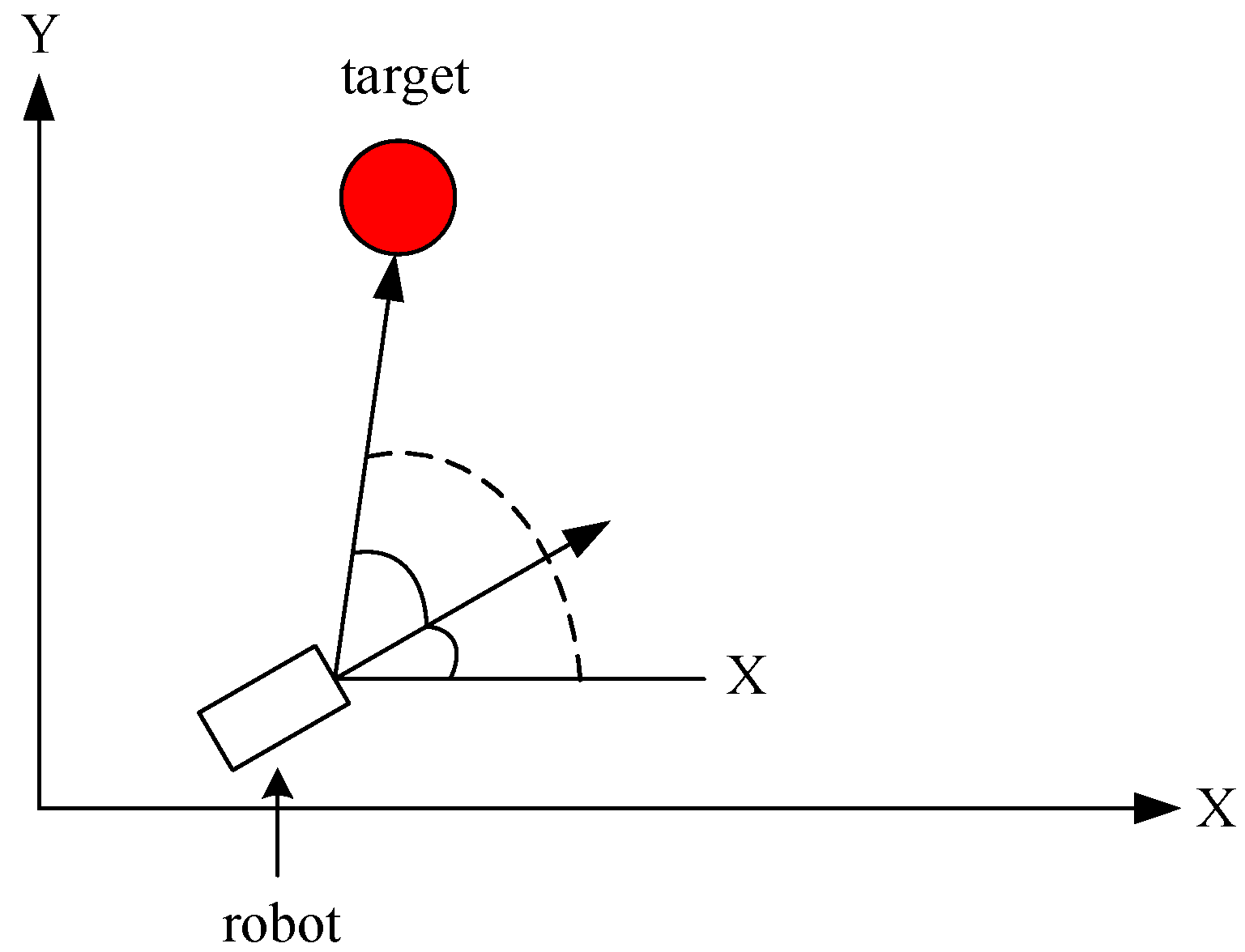
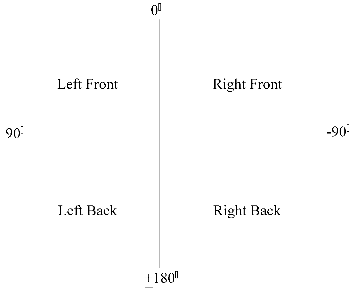
4. Navigation Control of a Mobile Robot

This study uses the AFNN mobile robot, which achieves navigation before requiring the goal and obstacle information. The eight sonar sensors are divided into three groups: Left, Front, and Right. In addition, we define the goal information ${\theta }_{tr}$, as shown in Figure 5. The four parameters control the input and enable mobile robot navigation. The AFNN output controls the speed of the robot’s left and right wheels. The parameters of AFNN is optimized through the MSABC in a training environment for the robot. Three targets are set on the training environment. Figure 6 shows angle between the mobile robot and target.

$$\mathrm{Left}=\begin{array}{cc}\min \left(S_i\right)& i=0,1\end{array}$$

(10)

$$\mathrm{Front}=\begin{array}{cc}\min \left(S_i\right)& i=2,3,4,5\end{array}$$

(11)

$$\mathrm{Right}=\begin{array}{cc}\min \left(S_i\right)& i=6,7\end{array}$$

(12)

$${\theta }_{tr}={\theta }_{target}-{\theta }_{robot}$$

(13)

where ${\theta }_{target}$ represents the angle between the target, and X coordinate and ${\theta }_{robot}$ represents the angle between the mobile robot and the X coordinate.

4.1. The Proposed Navigation Method

Most navigation methods are based on controlled parameters. In this study, a new evaluation function in MSABC is proposed for adjusting the control parameters without any training data. Figure 7 shows the navigation control process. The proposed function contains two control factors and three stop conditions. The three stop conditions are described as follows: (1) the robot collides with the obstacle; (2) the robot reaches the goal; (3) the robot navigates for time exceeding the user-defined time (i.e.,$T_{total}=T_{stop}^i$), where $T_{total}$ represents the mobile robot’s maximum navigation time step, which is user-defined according to the size of the environment, and $T_{stop}$ represents the mobile robot’s current navigation time step). The evaluation function is designed as follows:

$$f^i=\{\begin{array}{ccc}\frac{\frac{{\displaystyle \sum _{t=0}^{{}_{T_{stop}^i}}{d}_{act}^i\left(t\right)}}{d_{target}}}{T_{stop}^i-T_{stop}^{\min }+1},& & if{\displaystyle \sum _{t=0}^{{}_{T_{stop}^i}}{d}_{act}^i\left(t\right)}\le d_{target}\\ & & \\ \frac{\frac{d_{target}}{{\displaystyle \sum _{t=0}^{{}_{T_{stop}^i}}{d}_{act}^i\left(t\right)}}}{T_{stop}^i-T_{stop}^{\min }+1},& & Otherwise\end{array}$$

(14)

with

$$d_{act}^i(t)=\{\begin{array}{cc}\sqrt{{\left(R_x^i\left(t\right)-R_x^i\left(t-1\right)\right)}^2+{\left(R_y^i\left(t\right)-R_y^i\left(t-1\right)\right)}^2},& -90°\le {\theta }_{tr}\le 90°\\ -\sqrt{{\left(R_x^i\left(t\right)-R_x^i\left(t-1\right)\right)}^2+{\left(R_y^i\left(t\right)-R_y^i\left(t-1\right)\right)}^2},& else\end{array}$$

(15)

$$\begin{array}{cc}{T}_{stop}^{\min }=\min \left(T_{stop}^i\right),& i=1,2\dots ,M\end{array}$$

(16)

where t represents the time step of the mobile robot, i represents the number of controllers, M represents all numbers of controllers, $d_{act}^i$ represents the i_th mobile robot’s each time step taken toward the target, and $\left(R_x^i,R_y^i\left(t\right)\right)$ represents the i_th mobile robot’s time step of position, t. When ${\displaystyle \sum d_{act}^i\left(t\right)}$ equals the shortest distance of the target-evinced path, where the mobile robot reaches the target, because we need known positive or negative values of $d_{act}$. If $d_{act}^i>0$ represents the i_th mobile robot reaching the target, $d_{act}$ is a negative number representing the i_th mobile robot not reaching the target. Figure 8 shows the relation between $d_{target}$ and $d_{act}^i$.

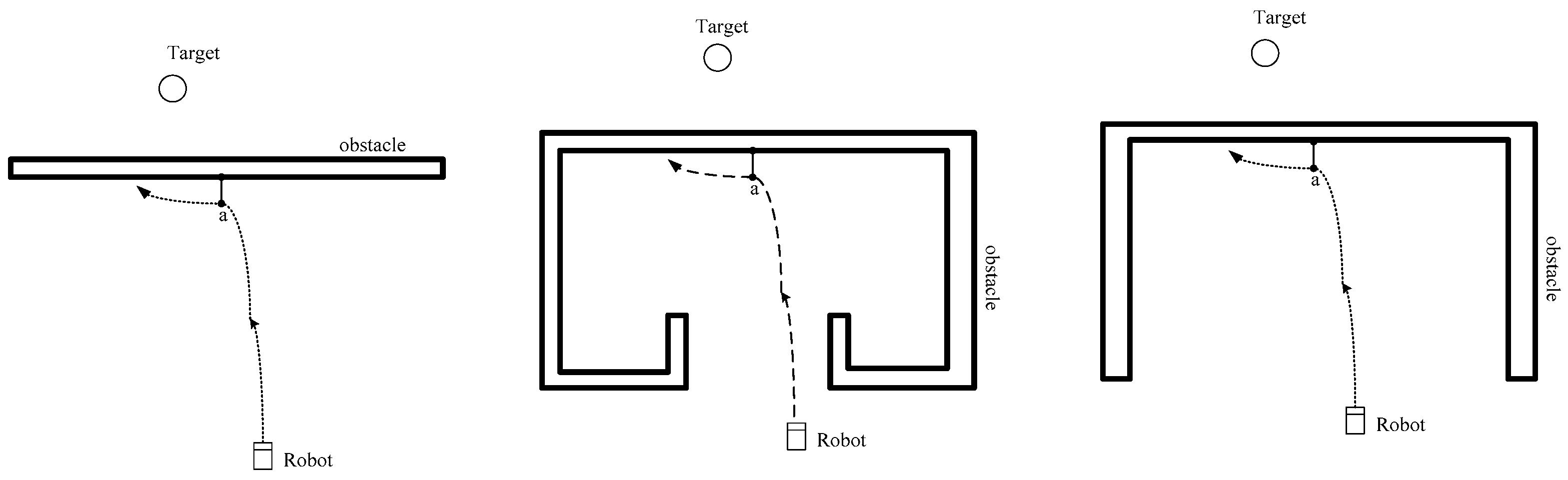
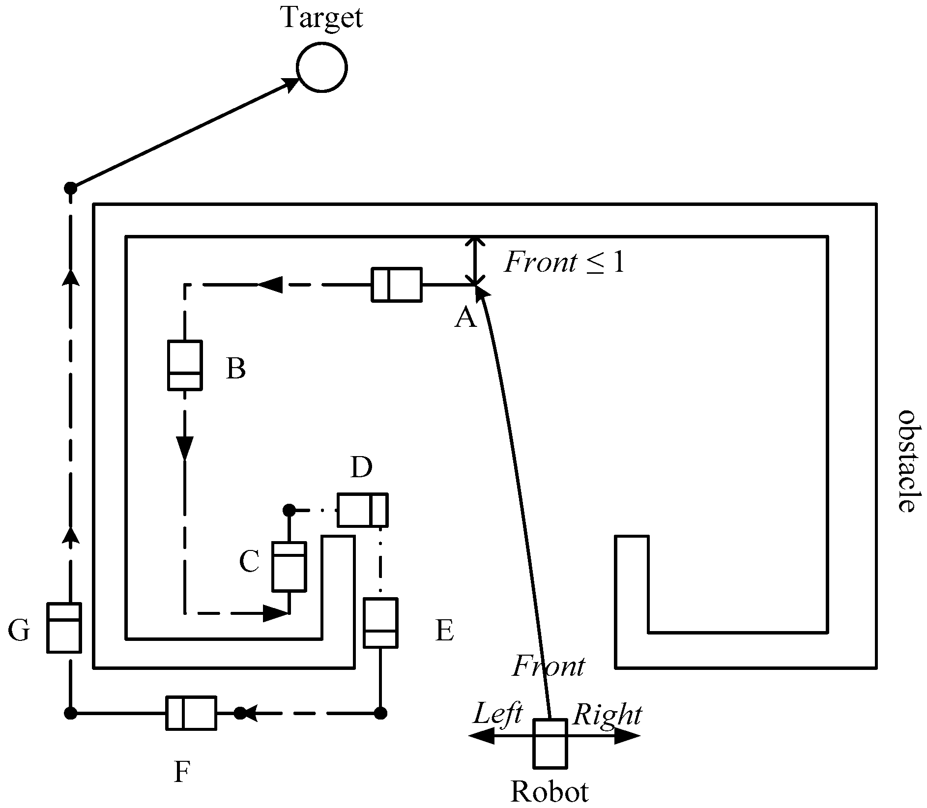
4.2. The Escape Method in Special Environments

In a complex environment, the mobile robot easily falls into traps, such as U-shaped obstacles. Therefore, a new escape method in a special environment is designed according to three U-shaped obstacles and shown in Figure 9. First, the direction of the mobile robot moving toward the target and the threshold value need to be defined. We divide the direction into four groups according to the angle between the mobile robot and target: Left-Front, Right-Front, Left-Back, and Right-Back, as shown in Figure 10. If Front is less than the threshold value, the mobile robot from the navigation behavior switches to the escape special environment behavior. The flowchart of the escape special environment behavior is shown in Figure 11.

In this study, a toward-left wall-following fuzzy logic controller (WF-FLC) is proposed. The inputs of a toward-left WF-FLC are the front obstacle distance Front and the right obstacle distance Right. The outputs are the left- and right-wheel speeds. The Front and Right inputs are divided into three linguistic terms: near, medium, and far. The membership function is shown in Figure 12a,b. The right and left wheels are divided into three linguistic terms: back, slow, medium, and fast. The membership function is shown in Figure 12c,d.

Table 1. The right-wheel rule table in the wall-following fuzzy logic controller (WF-FLC).

X′1 X′2	Near	Medium	Far
Near	Back	Fast	Fast
Medium	Fast	Medium	Medium
Far	Fast	Slow	Slow

and

Table 2. The left-wheel rule table in the WF-FLC.

X′1 X′2	Near	Medium	Far
Near	Back	Slow	Slow
Medium	Back	Medium	Medium
Far	Back	Fast	Fast

represent the left and right wheels designed in the toward-left WF-FLC using nine fuzzy rules. In this fuzzy rule table, a 0.5 m movement along the wall for the mobile robot is designed. The mobile robot turns right when the distance between mobile robot and the wall is far and turns left when the distance is close.

Figure 13 shows an example of escape special environment behavior. The mobile robot changes to the WF-FLC at point A. This turn-left count is set as one. The mobile robot reaches point B when the target is behind (including left back and right back) the robot. At this time, the mobile robot judges whether the left of the robot and no obstacle accounted with the turn-right count condition add to one. Moreover, the robot turns left from point A to point B, so the turn-left count adds to one. The mobile robot reaches point C when the turn-left count equals four. Finally, the mobile robot has already turned right four times at point G. Thus, the mobile robot changes the navigation behavior at point G.

5. Experimental Results

This section describes the Pinoneer3-DX implemented for navigation in an unknown environment and makes analysis between MSABC and other algorithms. First, the mobile robot application finds a new fitness function that evaluates the controller in the training environment and an optimal algorithm from the best controller, which helps mobile robot navigation in an unknown environment. Figure 5 shows the training environment.

Table 3. Initialization parameters before training.

Parameters	Values
Population size (PS)	30
Crossover rate (CR)	0.9
Scale factor (F)	0.5
Evaluation number	10,000
Number of rule	10
Scout bee limit	40
LP	50

shows the initial parameters for an optimal algorithm.

5.1. Performance Comparisons of Various Learning Algorithms

This study aims to analyze various learning algorithms for navigation control. Figure 14a–c show the robot trajectories of the proposed AFNN based on various learning algorithms. The mobile robot’s initial position is (1,1). The value of ${\theta }_{tr}$ changes in accordance with different targets in the training environment. The position of target one is (1,9), the distance between the start and target one is 8 m, and ${\theta }_{tr}$ is 53°; the position of target two is (9,9), the distance between the start and target two is 11.3 m, and ${\theta }_{tr}$ is 11°; and the position of target three is (9,5), the distance between the start and target three is 8.94 m, and ${\theta }_{tr}$ is 11°. Target one is a training mobile robot even if the neighbor obstacle interferes with the straight-reach target. Target two is a training mobile robot that avoids the obstacle after there is no obstacle around and toward the target movement. Target three is a training obstacle close to the target; the mobile robot also reaches the target. Figure 14a–c show that the mobile robot can overcome the problems of neighbor obstacle, no obstacle, and obstacle close to the target. Figure 14d shows the average value of the fitness function for the proposed MSABC design at each evaluation point and compares it with the corresponding values for the ABC and DE algorithm designs. It shows that the proposed MSABC design performs better than the ABC and DE algorithms in the navigation control.

Table 4. Performance comparison of the average fitness value using various learning algorithms.

Algorithms	MSABC	DE\Best1	DE\Best2	DE\Rand\Best\1	DE\Rand\Best\2	ABC
Average fitness f	2.362	2.173	1.796	2.112	1.9317	1.314
STD	0.16	0.387	0.2819	0.231	0.235	0.29

represents the standard deviation and mean of the fitness function f. An evaluation of the control function f of the MSABC, ABC, and DE algorithms in the training environment is given in

Table 5. Performance comparisons of the navigation time and the travel distance using various learning algorithms.

Algorithms	MSABC		DE\Best1
Evaluation Function	NavigationTime (s)	TravelDistance (m)	NavigationTime (s)	TravelDistance (m)
Target 1	9.184	7.8884	10.784	7.8508
Target 2	15.648	11.4683	17.248	11.4190
Target 3	14.6875	9.5638	16.0625	9.6121
Algorithms	DE\Best2		DE\Rand\Best\1
EvaluationFunction	NavigationTime (s)	TravelDistance (m)	NavigationTime (s)	TravelDistance (m)
Target 1	9.504	7.7824	9.76	7.7982
Target 2	16.416	11.3935	17.376	11.425
Target 3	15.75	9.6328	15.8125	9.6047
Algorithms	DE\Rand\Best\2		ABC
EvaluationFunction	NavigationTime (s)	TravelDistance (m)	NavigationTime (s)	TravelDistance (m)
Target 1	11.168	7.8614	12.256	7.501
Target 2	20.832	11.9809	24.96	10.8298
Target 3	19.625	11.1805	23.168	11.2815

.

In addition, this study will analyze the ultrasonic sensor values, the angle between mobile robot and target, and the left- and right-wheel speeds of the robot from start to target during the navigation control process. Here, take target three as an example. As shown in Figure 15a, the mobile robot reaches point A when it changes the navigation behavior to wall-following behavior until point B, which the mobile robot through escape special environment behavior judges the wall-following behavior end and changes to navigation behavior until point C. The mobile robot reaches point C after the left wheel is maintained at 0.84 m/s and the right wheel is maintained between 0.68 and 0.81 m/s back and forth. At this time, the mobile robot slowly turns right until reaching point D, where the Right value is below 0.36 m. The mobile robot has a left-wheel speed of 0.78 m/s and right-wheel speed of 0.82 m/s, and then slowly turns left to avoid the right obstacle. Then, it moves toward the target at point E. Figure 15b shows the distance values according to the ultrasonic sensors left, front, and right, the angle between mobile robot and target, and the left-wheel and right-wheel speeds of the robot at the robot moving distances.

5.2. Verification of Mobile Robot Escape in Special Environments

This subsection designs three special environments, proving the ability of the mobile robot to escape the special environment. Figure 16 show the local minima of the traditional environments. The first one is a V-shaped environment, second is a U-shaped environment, and third is a several-obstacle environment. Finally, the mobile robot can escape the special environment and reach the target.

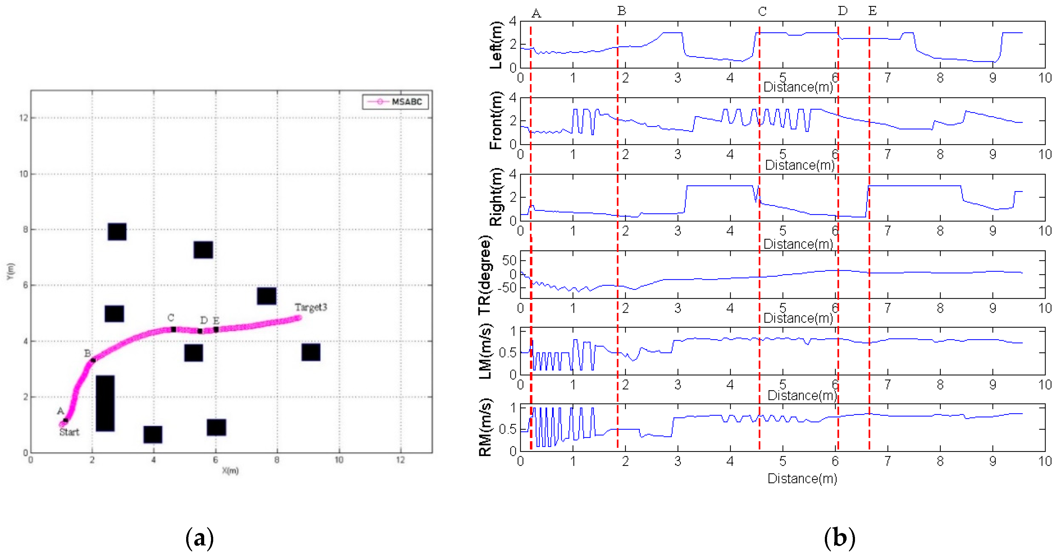
5.3. PIONEER 3-DX Robot Navigation

In the experiments, an actual mobile robot navigation control using the AFNN based on MSABC algorithm, as well as a PIONEER 3-DX robot, is conducted. To demonstrate the feasibility of the AFNN based on MSABC algorithm, a real environment is created to test the robot’s performance in an actual navigation task. The PIONEER3-DX robot reaches a maximum translation speed of 1.2 m/s. Figure 17 shows images of the navigation control results for the proposed approach. The PIONEER 3-DX robot can reach the target, but with a distance of 30 cm between the target and robot stop point.

6. Conclusions

This study proposes an AFNN based on MSABC algorithm for achieving an actual mobile robot navigation control and escape special environment behavior to avoid special obstacles. During the navigation control process, the AFNN inputs measure the distance between the ultrasonic sensors and angle between the mobile robot and target, and the outputs are the robot’s left- and right-wheel speeds. A fitness function is defined to evaluate the AFNN performance in the navigation control. The fitness function includes the following three control factors: navigation time, distance between the start and the target, and distance between the mobile robot and target travelled. The traditional ABC algorithm simulates the intelligent foraging behavior of honey-bee swarms, which are good at exploration but poor at exploitation. The proposed MSABC algorithm adopts the mutation strategies of a differential evolution to balance exploration and exploitation. The experimental results show that the proposed MSABC method has improved the performance of average fitness, navigation time, and travel distance by 79.75%, 33.03%, and 10.74%, respectively, compared with the traditional ABC method. In order to prove the feasibility of the design, experiments were carried out on the actual PIONEER 3-DX mobile robot, and the navigation control was successfully completed.

References

1. Seraji, H.; Howard, A. Behavior-based robot navigation on challenging terrain: A fuzzy logic approach. IEEE Trans. Robot. Autom. 2002, 18, 308–321. [Google Scholar] [CrossRef] [Green Version]
2. Abdessemed, F.; Benmahammed, K.; Monacelli, E. A fuzzy-based reactive controller for a non-holonomic mobile robot. Robot. Auton. Syst. 2004, 47, 31–46. [Google Scholar] [CrossRef]
3. Pratihar, D.K.; Deb, K.; Ghosh, A. A genetic-fuzzy approach for mobile robot navigation among moving obstacles. Int. J. Approx. Reason. 1999, 20, 145–172. [Google Scholar] [CrossRef] [Green Version]
4. Boubertakh, H.; Tadjine, M.; Glorennec, P.Y. A new mobile robot navigation method using fuzzy logic and a modified Q-learning algorithm. J. Intell. Fuzzy Syst. 2010, 21, 113–119. [Google Scholar] [CrossRef]
5. Juang, C.F.; Chang, Y.C. Evolutionary-group-based particle-swarm-optimized fuzzy controller with application to mobile-robot navigation in unknown environments. IEEE Trans. Fuzzy Syst. 2011, 19, 379–392. [Google Scholar] [CrossRef]
6. Yang, J.; Zhuang, Y.; Li, C. Towards behavior control for evolutionary robot based on RL with ENN. Int. J. Adv. Robot. Syst. 2012, 10, 157. [Google Scholar] [CrossRef]
7. Nakhaeinia, D.; Karasfi, B. A behavior-based approach for collision avoidance of mobile robots in unknown and dynamic environments. J. Intell. Fuzzy Syst. 2013, 24, 299–311. [Google Scholar] [CrossRef]
8. Mohanty, P.K.; Parhi, D.R. A new intelligent motion planning for mobile robot navigation using multiple adaptive neuro-fuzzy inference system. Appl. Math. Inf. Sci. 2014, 8, 2527–2535. [Google Scholar] [CrossRef] [Green Version]
9. Eiben, A.E.; Hinterding, R.; Michalewicz, Z. Parameter control in evolutionary algorithms. IEEE Trans. Evol. Comput. 1999, 3, 124–141. [Google Scholar] [CrossRef] [Green Version]
10. Hu, Y.; Zheng, J.; Zou, J.; Yang, S.; Ou, J. A dynamic multi-objective evolutionary algorithm based on intensity of environmental change. Inf. Sci. 2020, 523, 49–62. [Google Scholar] [CrossRef]
11. Cordon, O.; Gomide, F.; Herrera, F.; Hoffmann, F.; Magdalena, L. Ten years of genetic fuzzy systems: Current framework and new trends. Fuzzy Sets Syst. 2004, 141, 5–31. [Google Scholar] [CrossRef]
12. Kong, F.; Jiang, J.; Huang, Y. An Adaptive Multi-Swarm Competition Particle Swarm Optimizer for Large-Scale Optimization. Mathematics 2019, 7, 521. [Google Scholar] [CrossRef] [Green Version]
13. Elaziz, M.A.; Li, L.; Jayasena, K.P.N.; Xiong, S. Multiobjective big data optimization based on a hybrid salp swarm algorithm and differential evolution. Appl. Math. Model. 2020, 80, 929–943. [Google Scholar] [CrossRef]
14. Weile, D.S.; Michielssen, E. Genetic algorithm optimization applied to electromagnetics: A review. IEEE Trans. Antennas Propag. 1997, 45, 343–353. [Google Scholar] [CrossRef]
15. Coelho, L.D.S.; Herrera, B.M. Fuzzy identification based on a chaotic particle swarm optimization approach applied to a nonlinear yo-yo motion system. IEEE Trans. Ind. Electron. 2007, 54, 3234–3324. [Google Scholar] [CrossRef]
16. Wai, R.J.; Lee, J.D.; Chuang, K.L. Real-time PID control strategy for maglev transportation system via particle swarm optimization. IEEE Trans. Ind. Electron. 2011, 58, 629–646. [Google Scholar] [CrossRef]
17. Price, K.V.; Storn, R.M.; Lampinen, J.A. Differential Evolution: A Practical Approach to Global Optimization; Springer-Verlag: Berlin, Germany, 2005. [Google Scholar]
18. Rahnamayan, S.; Tizhoosh, H.R.; Salama, M.M.A. Opposition-based differential evolution. IEEE Trans. Evol. Comput. 2008, 12, 107–125. [Google Scholar] [CrossRef] [Green Version]
19. Wang, Y.; Cai, Z.X.; Zhang, Q.F. Differential evolution with composite trial vector generation strategies and control parameters. IEEE Trans. Evol. Comput. 2011, 15, 55–66. [Google Scholar] [CrossRef]
20. Das, S.; Suganthan, P.N. Differential evolution: A survey of the state-of-the-art. IEEE Trans. Evol. Comput. 2011, 15, 4–31. [Google Scholar] [CrossRef]
21. Yang, X.S. Engineering optimizations via nature-inspired virtual bee algorithms. Lect. Notes Comput. Sci. 2005, 3562, 317–323. [Google Scholar]
22. Pham, D.T.; Ghanbarzadeh, A.; Koc, E.; Otri, S.; Rahim, S.; Zaidi, M. The Bees Algorithm, Technical Report; Manufacturing Engineering Centre, Cardiff University: Cardiff, UK, 2005. [Google Scholar]
23. Karaboga, D. An Idea Based on Honeybee Swarm for Numerical Optimization; Computer Engineering Department, Engineering Faculty, Erciyes University: Talas/Kayseri, Turkey, 2005. [Google Scholar]
24. Karaboga, D.; Basturk, B. A powerful and efficient algorithm for numerical function optimization: Artificial bee colony (ABC) algorithm. J. Glob. Optim. 2007, 39, 459–471. [Google Scholar] [CrossRef]
25. Karaboga, D.; Basturk, B. On the performance of artificial bee colony (ABC) algorithm. Appl. Soft Comput. 2008, 8, 687–697. [Google Scholar] [CrossRef]
26. Lin, T.C.; Chen, C.C.; Lin, C.J. Wall-following and navigation control of mobile robot using reinforcement learning based on dynamic group artificial bee colony. J. Intell. Robot. Syst. 2018, 92, 343–357. [Google Scholar] [CrossRef]
27. Karaboga, D.; Gorkemli, B. Solving traveling salesman problem by using combinatorial artificial bee colony algorithms. Int. J. Artif. Intell. Tools 2019, 28, 1950004. [Google Scholar] [CrossRef]
28. Karaboga, D.; Aslan, S. Discovery of conserved regions in DNA sequences by artificial bee colony (ABC) algorithm based methods. Nat. Comput. 2019, 18, 333–350. [Google Scholar] [CrossRef]
29. Karaboga, D.; Kaya, E. Training ANFIS by using an adaptive and hybrid artificial bee colony algorithm (aABC) for the identification of nonlinear static systems. Arab. J. Sci. Eng. 2019, 44, 3531–3547. [Google Scholar] [CrossRef]
30. Chen, C.H. An efficient compensatory neuro-fuzzy system and its applications. Int. J. Gen. Syst. 2012, 41, 353–371. [Google Scholar] [CrossRef]
Figure 1. (a) Pioneer 3-DX, (b) Sonar sensor position.
Mathematics 08 01223 g001
Figure 2. Structure of the adaptive fuzzy neural network (AFNN).
Mathematics 08 01223 g002
Figure 3. Flowchart of the multi-strategy artificial bee colony (MSABC) algorithm.
Mathematics 08 01223 g003
Figure 4. Rule-coded solution in MSABC.
Mathematics 08 01223 g004
Figure 5. Illustration of the training environment.
Mathematics 08 01223 g005
Figure 6. Illustration of angle θ t r between the mobile robot and target.
Mathematics 08 01223 g006
Figure 7. Illustration of the navigation control process.
Mathematics 08 01223 g007
Figure 8. The relation between dtarget and dact.
Mathematics 08 01223 g008
Figure 9. Special environments.
Mathematics 08 01223 g009
Figure 10. The direction between target and θ t r .
Mathematics 08 01223 g010
Figure 11. Flowchart of the escape method in special environments.
Mathematics 08 01223 g011
Figure 12. (a) The front sensor value of the robot, (b) The right sensor value of the robot, (c) Left-wheel speed of the robot, (d) Right-wheel speed of the robot.
Mathematics 08 01223 g012
Figure 13. An example of escape special environment behavior.
Mathematics 08 01223 g013
Figure 14. Comparisons of robot trajectories from start to different targets in the training environment using various learning algorithms.
Mathematics 08 01223 g014
Figure 15. (a) Robotic trajectories using an AFNN based on MSABC algorithm; and (b) the ultrasonic sensor values, the angle between mobile robot and target three, and the left- and right-wheel speeds of the robot from start to target three.
Mathematics 08 01223 g015
Figure 16. (a) V-shaped environment; (b) U-shaped environment; and (c) Multi-obstacle environment.
Mathematics 08 01223 g016
Figure 17. Navigation control results of PIONEER 3-DX in an actual environment using the AFNN based on MSABC algorithm.
Mathematics 08 01223 g017