On Partial Stochastic Comparisons Based on Tail Values at Risk

Abstract

The tail value at risk at level p, with $p\in (0,1),$ is a risk measure that captures the tail risk of losses and asset return distributions beyond the p quantile. Given two distributions, it can be used to decide which is riskier. When the tail values at risk of both distributions agree, whenever the probability level $p\in (0,1),$ about which of them is riskier, then the distributions are ordered in terms of the increasing convex order. The price to pay for such a unanimous agreement is that it is possible that two distributions cannot be compared despite our intuition that one is less risky than the other. In this paper, we introduce a family of stochastic orders, indexed by confidence levels $p_0\in (0,1),$ that require agreement of tail values at risk only for levels $p>p_0$. We study its main properties and compare it with other families of stochastic orders that have been proposed in the literature to compare tail risks. We illustrate the results with a real data example.

1. Motivation and Preliminaries

In actuarial and financial sciences, risk managers and investors dealing with insurance losses and asset returns are often concerned with the right-tail risk of distributions, which is related to large deviations due to the right-tail losses or right-tail returns (see Wang [1]). To compare the risk associated to different models, they use risk measures typically based on quantiles, such as the value at risk, the tail value at risk and some generalizations of these measures (see the book by Guégan and Hassani [2] for a recent review on the topic of risk measurement). Comparisons of two quantile-based risk measures made for a particular confidence level p are not very informative (they are based on two single numbers) and a change in the confidence level may produce different conclusions. An alternative method to compare two risks X and Y is to use stochastic orderings, which conclude that X is smaller than Y when a family of risk measures (rather than a single risk measure) agrees in the conclusion that X is less risky than $Y.$ For example, the increasing convex order (which is formally defined below) requires agreement of tail values at risk for any confidence level $p\in (0,1)$. An advantage of this method is, obviously, its robustness toward changes in the confidence level, which can be interpreted in terms of a common agreement of different decision-maker’s attitudes. By robustness, we understand how sensitive the comparison procedure to different values of p is. For other interpretations of robustness in risk measurement, see Zhelonkin and Chavez-Demoulin [3]. However, this approach has the drawback that some distributions cannot be compared despite our intuition that one is less risky than the other.

One way to increase the number of distributions that can be compared without losing robustness is to reduce the range of values of the confidence level p required to reach an agreement. For example, an investor concerned with right-tail risks may think that X is less risky than Y if the respective tail values at risk agree in the conclusion that X is less risky than Y for any confidence level p such that $p>p_0,$ where $p_0\in (0,1)$ is chosen to suit his/her specific preferences. The aim of this paper is precisely to study a family of stochastic orders based on such an agreement.

Let X be a random variable describing losses of a financial asset and let F be its distribution function (as usual, negative losses are gains). The value at risk of X at level $p\in (0,1),$ or p-quantile, is defined by

$$\mathrm{Va}{\mathrm{R}}_p\left[X\right]=F^{-1}\left(p\right)=inf\{x:F\left(x\right)\ge p\},\mathrm{for}\mathrm{all}p\in (0,1).$$

(1)

For a given $p\in (0,1)$, $\mathrm{Va}{\mathrm{R}}_p\left[X\right]$ represents the maximum loss the investor can suffer with $100p\%$ confidence over a certain period of time. Despite being widely used in practice, VaR has two major drawbacks. First, it does not describe the tail behavior beyond the confidence level. Second, VaR is not, in general, subadditive (except in some special cases; for example, when the underlying distribution belongs to the elliptical family of distributions, the estimator of VaR is subadditive). The literature offers different possible alternatives to overcome the limitations of VaR (see, for example, Ahmadi-Javid [4]). One of the most important is the tail value at risk or $\mathrm{TVaR}$, defined by

$$\mathrm{TVa}{\mathrm{R}}_p\left[X\right]={\displaystyle \frac{1}{1-p}}{\int }_p^1{F}^{-1}\left(u\right)du,\mathrm{for}\mathrm{all}p\in [0,1).$$

TVaR is subadditive (that is, $\mathrm{TVa}{\mathrm{R}}_p[X+Y]\le \mathrm{TVa}{\mathrm{R}}_p\left[X\right]+\mathrm{TVa}{\mathrm{R}}_p\left[Y\right]$ for all losses X and Y). Given $p\in (0,1)$ and X continuous, $\mathrm{TVa}{\mathrm{R}}_p\left[X\right]$ represents the average loss when losses exceed $\mathrm{TVa}{\mathrm{R}}_p\left[X\right]$.

In this paper, we study the following family of stochastic orders indexed by confidence levels $p_0\in [0,1).$

Definition 1.

Let X and Y be two random variables and $p_0\in [0,1)$. Then, X is said to be smaller than Y in the $p_0$-tail value at risk order, denoted by $X{\le }_{p_0-\mathrm{tvar}}Y$, if

$$\mathrm{TVa}{\mathrm{R}}_p\left(X\right)\le \mathrm{TVa}{\mathrm{R}}_p\left(Y\right),forallp>p_0.$$

(2)

When (2) holds for $p_0=0$, then we have the usual increasing convex order (see Lemma 2.1 in Sordo and Ramos [5]) and we denote $X{\le }_{icx}Y$. The books by Shaked and Shanthikumar [6] and Belzunce et al. [7] collect many properties and applications of the increasing convex order. If $X{\le }_{\mathrm{icx}}Y$, then X is both smaller (in fact, $X{\le }_{icx}Y$ implies $\mathrm{E}\left[X\right]\le \mathrm{E}\left[Y\right]$) and less variable than $Y.$ In finance and insurance, the increasing convex order is often interpreted in terms of stop-loss contracts and it is also called stop-loss order. Specifically, it holds that $X{\le }_{\mathrm{icx}}Y$ if, and only if,

$$\mathrm{E}\left[{(X-x)}_{+}\right]\le \mathrm{E}\left[{(Y-x)}_{+}\right],\mathrm{for}\mathrm{all}x\in \mathbb{R},$$

(3)

where ${\left(x\right)}_{+}=x$, if $x\ge 0$ and ${\left(x\right)}_{+}=0$, if $x<0$, or, equivalently, if

$${\int }_x^{+\infty }\overline{F}\left(t\right)dt\le {\int }_x^{+\infty }\overline{G}\left(t\right)dt,\mathrm{for}\mathrm{all}x\in \mathbb{R},$$

(4)

provided the integrals exist, where $\overline{F}=1-F$ and $\overline{G}=1-G$ are the tail functions of X and Y, respectively. One purpose of this paper is to study how these characterizations change when the order $X{\le }_{\mathrm{icx}}Y$ is replaced by the weaker $X{\le }_{p_0-\mathrm{tvar}}Y,$ for some $p_0>0$.

We provide an analytical example to motivate the study of the new family of stochastic orders. Let us consider two Pareto loss distributions $X\sim P(7,3)$ and $Y\sim P(3,2)$. The value at risk of a Pareto distribution $Z\sim P(a,k)$, with shape parameter $a>0$ and scale parameter $k\in \mathbb{R}$, is given by

$$F_Z^{-1}\left(p\right)=\frac{k}{{(1-p)}^{\frac{1}{a}}},\mathrm{for}\mathrm{all}p\in (0,1),$$

and, if $a>1,$ the expectation is $\mathrm{E}\left[Z\right]=ak/(a-1)$. Figure 1 shows the plot of the quantile functions for X and Y. Since $\mathrm{E}\left[X\right]=3.5>3=\mathrm{E}\left[Y\right]$, then $X{\nleqq }_{icx}Y$.

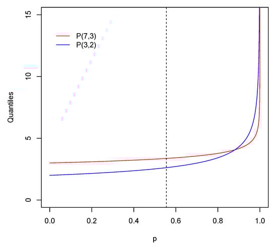
Figure 1. Quantile functions for $X\sim P(7,3)$ and $Y\sim P(3,2)$.

However, it can be checked that $\mathrm{TVa}{\mathrm{R}}_p\left(X\right)\le \mathrm{TVa}{\mathrm{R}}_p\left(Y\right)$, for all $p\ge 0.55482$ where here $p_0=0.55482$ is the minimum value such that $X{\le }_{p_0-\mathrm{tvar}}Y$ ($p_0$ is represented with a dashed line in Figure 1). An investor concerned with large deviations due to the right-tail losses may make decisions based on the tail value at risk for large values of p. If this is the case, he/she will evaluate X as less dangerous than $Y,$ despite $\mathrm{E}\left[X\right]>\mathrm{E}\left[Y\right]$ and $X{\nleqq }_{\mathrm{icx}}Y$.

The idea of limiting the number of comparisons to weaken the increasing convex order is not new. Given two random variables X and Y with the same mean, Cheung and Vanduffel [8] say that X is smaller than Y in the tail convex order with index $x_0\in \mathbb{R}$ (denoted by $X{\le }_{\mathrm{tcx}\left(x_0\right)}Y$) if

$$\mathrm{E}\left[{(X-x)}_{+}\right]\le \mathrm{E}\left[{(Y-x)}_{+}\right],\mathrm{for}\mathrm{all}x\ge x_0.$$

(5)

According to (3), if X and Y have the same mean, then $X{\le }_{\mathrm{tcx}(-\infty )}Y$ is the same as $X{\le }_{icx}Y.$ It is natural to wonder, when $E\left[X\right]=E\left[Y\right]$, about the relationship between $X{\le }_{p_0-\mathrm{tvar}}Y$ and $X{\le }_{\mathrm{tcx}\left(x_0\right)}Y.$ We address this issue below.

For other recent studies of orders based on tail comparisons see Sordo et al. [9], Mulero et al. [10] and Belzunce et al. [11].

The rest of the work is organized as follows. In Section 2, we study the main properties of the order ${\le }_{p_0-\mathrm{tvar}}$ and find sufficient conditions under which it holds. We also investigate its relationships with other well-known stochastic orders and compare parametric families of distributions. In particular, we relate the order ${\le }_{p_0-\mathrm{tvar}}$ to the notion of pure tail order as considered by Rojo [12]. In Section 3 we illustrate the applicability of the new family of orders using a real dataset. Section 4 contains conclusions.

Throughout the paper, “increasing” means “non-decreasing” and “decreasing” means “non-increasing”. Random variables are assumed to have finite means. Given a function h, $S^{-}\left(h\right)$ denotes the number of sign changes of h on its support, where zero terms are discarded.

2. Properties and Relationships with Other Stochastic Orders

It is trivially verified that $X{\le }_{p_0-\mathrm{tvar}}X$ for all $p_0\in (0,1)$ and that $X{\le }_{p_0-\mathrm{tvar}}Y$ for $p_0\in (0,1)$ implies $X{\le }_{q_0-\mathrm{tvar}}Y$, for all $q_0\in [p_0,1)$. It is also obvious that if X, Y and Z are three random variables such that $X{\le }_{p_0-\mathrm{tvar}}Y$ and $Y{\le }_{p_1-\mathrm{tvar}}Z$ with $p_0,p_1\in (0,1)$, then $X{\le }_{p_3-\mathrm{tvar}}Z$ with $p_3=max\{p_0,p_1\}$. Finally, if $X{\le }_{p_0-\mathrm{tvar}}Y$ and $Y{\le }_{p_1-\mathrm{tvar}}X$, with $p_0,p_1\in (0,1)$, then $\mathrm{TVa}{\mathrm{R}}_p\left(X\right)=\mathrm{TVa}{\mathrm{R}}_p\left(Y\right)$, for all $p\in [p_3,1]$, where $p_3$ is defined as before.

Next, we provide some closure properties. In particular, we point out the closure under convergence in distribution and under increasing convex transformations. First of all, recall that given a sequence of random variables $\{X_n:n=1,2,\dots \}$ with distribution functions $F_n$ and F, respectively, then $X_n$ is said to converge in distribution to X, denoted by $X_n\stackrel{\mathit{d}}{⟶}X$, if ${lim}_{n\to +\infty }{F}_n\left(x\right)=F\left(x\right)$ for all x at which F is continuous.

Proposition 1.

Let $\{X_n:n=1,2,\dots \}$ and $\{Y_n:n=1,2,\dots \}$ be two sequences of positive continuous random variables such that $X_n\stackrel{\mathrm{d}}{⟶}X$ and $Y_n\stackrel{\mathrm{d}}{⟶}Y$. Assume that $X_n$ and X have a common interval support for all $n\in \mathbb{N}$ and ${lim}_{n\to \infty }\mathrm{E}\left[X_n\right]=\mathrm{E}\left[X\right]$ (and, analogously, for $Y_n$ and Y and their expectations). If $X_n{\le }_{p_0-\mathrm{tvar}}{Y}_n$ for $p_0\in (0,1)$, then $X{\le }_{p_0-\mathrm{tvar}}Y$.

Proof. 

From Definition 1, it is clear that $X{\le }_{p_0-\mathrm{tvar}}Y$ if, and only if,

$${\int }_p^1{F}^{-1}\left(u\right)du\le {\int }_p^1{G}^{-1}\left(u\right)du,\mathrm{for}\mathrm{all}p\ge p_0.$$

(6)

Integration by parts in (6) shows that

$$X{\le }_{p_0-\mathrm{tvar}}Y⟺{\int }_{F^{-1}\left(p\right)}^{+\infty }\overline{F}\left(t\right)dt+F^{-1}\left(p\right)(1-p)\le {\int }_{G^{-1}\left(p\right)}^{+\infty }\overline{G}\left(t\right)dt+G^{-1}\left(p\right)(1-p),p\ge p_0.$$

(7)

Now, from $X_n\stackrel{\mathrm{d}}{⟶}X$, we have that

$$\underset{n\to +\infty }{lim}{F}_n^{-1}\left(p\right)=F^{-1}\left(p\right),$$

(8)

for all point p where $F^{-1}$ is continuous, where $F_n$ and F are the distribution functions of $X_n$ and X, respectively (see, for example, Chapter 21 in Van der Vaart [13]). Moreover, from Theorem 2.3 in Müller [14], it holds that

$$\underset{n\to +\infty }{lim}{\int }_x^{+\infty }{\overline{F}}_n\left(t\right)dt={\int }_x^{+\infty }\overline{F}\left(t\right)dt,\mathrm{for}\mathrm{all}x\in \mathbb{R}.$$

(9)

Using the dominated convergence theorem, it follows from (8) and (9) that

$$\underset{n\to +\infty }{lim}\left[{\int }_{F_n^{-1}\left(p\right)}^{+\infty }{\overline{F}}_n\left(t\right)dt+F_n^{-1}\left(p\right)(1-p)\right]={\int }_{F^{-1}\left(p\right)}^{+\infty }\overline{F}\left(t\right)dt+F^{-1}\left(p\right)(1-p).$$

(10)

From $Y_n\stackrel{\mathrm{d}}{⟶}Y$ we see that (10) also holds when G and $G_n$ replace, respectively, F and $F_n$. Now the result follows from (7). □

The closure under strictly increasing convex transformations require the following lemma taken from page 120 in Barlow and Proschan [15].

Lemma 1.

Let W be a measure on the interval $(a,b)$, not necessarily nonnegative. Let h be a nonnegative function defined on $(a,b)$. If ${\int }_t^{b}dW\left(x\right)\ge 0$ for all $t\in (a,b)$ and if h is increasing, then ${\int }_a^{b}h\left(x\right)dW\left(x\right)\ge 0$.

Proposition 2.

Let X and Y be two random variables and let ϕ be a strictly increasing and convex function. If $X{\le }_{p_0-\mathrm{tvar}}Y$ for $p_0\in (0,1)$, then $\varphi \left(X\right){\le }_{p_0-\mathrm{tvar}}\varphi \left(Y\right)$.

Proof. 

Let $F_{\varphi }$ and $G_{\varphi }$ denote the distribution functions of $\varphi \left(X\right)$ and $\varphi \left(Y\right)$, respectively. Since $\varphi$ is strictly increasing we see that $F_{\varphi }^{-1}\left(p\right)=\varphi \left(F^{-1}\left(p\right)\right)$ and $G_{\varphi }^{-1}\left(p\right)=\varphi \left(G^{-1}\left(p\right)\right)$, for all $p\in (0,1)$. Since $\varphi$ is convex, we know (see, for example, Theorem 10.11 in Zygmund [16]) that there exists an increasing function $\phi$ such that

$$\varphi \left(G^{-1}\left(u\right)\right)-\varphi \left(F^{-1}\left(u\right)\right)={\int }_{F^{-1}\left(u\right)}^{G^{-1}\left(u\right)}\phi \left(v\right)dv.$$

Moreover, since $\varphi$ is strictly increasing, the function $\phi$ is positive (in fact, it is the derivative of $\varphi$ except, perhaps, at some singular points). Observe that if $F^{-1}\left(u\right)\le G^{-1}\left(u\right)$, then

$${\int }_{F^{-1}\left(u\right)}^{G^{-1}\left(u\right)}\phi \left(v\right)dv\ge \phi \left(F^{-1}\left(u\right)\right)\left[G^{-1}\left(u\right)-F^{-1}\left(u\right)\right],$$

and, if $F^{-1}\left(u\right)>G^{-1}\left(u\right)$, then

$${\int }_{F^{-1}\left(u\right)}^{G^{-1}\left(u\right)}\phi \left(v\right)dv=-{\int }_{G^{-1}\left(u\right)}^{F^{-1}\left(u\right)}\phi \left(v\right)dv\ge \phi \left(F^{-1}\left(u\right)\right)\left[G^{-1}\left(u\right)-F^{-1}\left(u\right)\right].$$

Therefore, we have that

$$\begin{array}{ccc}\hfill {\int }_p^1\left[\varphi \left(G^{-1}\left(u\right)\right)-\varphi \left(F^{-1}\left(u\right)\right)\right]du& =& {\int }_p^1\left({\int }_{F^{-1}\left(u\right)}^{G^{-1}\left(u\right)}\phi \left(v\right)dv\right)du\hfill \\ \hfill & \ge & {\int }_p^1\phi \left(F^{-1}\left(u\right)\right)\left[G^{-1}\left(u\right)-F^{-1}\left(u\right)\right]du\ge 0,\hfill \end{array}$$

where the last inequality follows from (6) and Lemma 1 using the fact that the function $\phi \left(F^{-1}\left(u\right)\right)I(p<u)$ is positive and increasing. Consequently,

$${\int }_p^1\varphi \left(F^{-1}\left(u\right)\right)\le {\int }_p^1\varphi \left(F^{-1}\left(u\right)\right)du,$$

for all $p\ge p_0$, which means $\varphi \left(X\right){\le }_{p_0-\mathrm{tvar}}\varphi \left(Y\right)$. □

Next, we give the following relationship among the new order and the icx order of certain random variables.

Proposition 3.

Let X and Y be two random variables. If

$$max\left\{X,F^{-1}\left(p_0\right)\right\}{\le }_{\mathrm{icx}}max\left\{Y,G^{-1}\left(p_0\right)\right\},$$

then $X{\le }_{p_0-\mathrm{tvar}}Y$.

Proof. 

Given a random variable X with distribution function F, let

$$X_0=max\left\{X,F^{-1}\left(p_0\right)\right\},p_0\in (0,1),$$

and let $F_0^{-1}$ be its corresponding quantile function, given by

$$F_0^{-1}\left(p\right)=\left\{\begin{array}{cc}{F}^{-1}\left(p_0\right),\hfill & \mathrm{if}0<p<p_0,\hfill \\ F^{-1}\left(p\right),\hfill & \mathrm{if}{p}_0\le p<1.\hfill \end{array}\right.$$

(11)

A straightforward computation gives

$${\mathrm{TVaR}}_p\left(X_0\right)=\left\{\begin{array}{cc}\frac{1}{1-p}\left({\int }_{p_0}^1{F}^{-1}\left(u\right)du+F^{-1}\left(p_0\right)(p_0-p)\right),\hfill & \mathrm{if}0<p<p_0,\hfill \\ \frac{1}{1-p}{\int }_p^1{F}^{-1}\left(u\right)du={\mathrm{TVaR}}_p\left(X\right),\hfill & \mathrm{if}{p}_0\le p<1.\hfill \end{array}\right.$$

(12)

We obtain similarly ${\mathrm{TVaR}}_p\left(Y_0\right),$ where $Y_0$ is analogously defined to $X_0$. It is clear than ${\mathrm{TVaR}}_p\left(X_0\right)\le {\mathrm{TVaR}}_p\left(Y_0\right)$ for all $p\in (0,1)$ implies ${\mathrm{TVaR}}_p\left(X\right)\le {\mathrm{TVaR}}_p\left(Y\right)$ for $p_0\le p<1$, which proves the result. □

Remark 1.

A stop-loss order is defined as the maximum loss that an investor assumes on a particular investment. Given a loss random variable X, the random variable $max\left\{X,F^{-1}\left(p_0\right)\right\}$ can be interpreted as a stop-loss order at $F^{-1}\left(p_0\right).$

Next we discuss the connections between the $p_0$-tail value at risk order and the tail convex order defined by (5). Observe that $X{\le }_{tcx\left(x_0\right)}Y$ if $E\left[X\right]=E\left[Y\right]$ and

$${\int }_x^{+\infty }\overline{F}\left(t\right)dt\le {\int }_x^{+\infty }\overline{G}\left(t\right)dt,\forall x\ge x_0.$$

(13)

With our notation, given X and Y such that $E\left[X\right]=E\left[Y\right],$ Theorem 4 of Cheung and Lo [17] shows that $X{\le }_{p_0-\mathrm{tvar}}Y$ for $p_0\in (0,1)$ implies $X{\le }_{\mathrm{tcx}\left(F^{-1}\left(p_0\right)\right)}Y$ and that $X{\le }_{\mathrm{tcx}\left(x_0\right)}Y$ for $x_0\in \mathbb{R}$ implies $X{\le }_{G\left(x_0\right)-\mathrm{tvar}}Y$ and $X{\le }_{\mathrm{tcx}(F^{-1}\left(G\left(x_0\right)\right)}Y$.

Remark 2.

Given X and Y with the same mean, a natural question is whether $X{\le }_{p_0-\mathrm{tvar}}Y$ for $p_0\in (0,1)$ implies $X{\le }_{\mathrm{tcx}\left(x_0\right)}Y$ for $x_0<F^{-1}\left(p_0\right)$. In general, the answer is no. Let us assume that $X{\le }_{p_0-\mathrm{tvar}}Y$ for $p_0\in (0,1)$ such that $G^{-1}\left(p_0\right)<F^{-1}\left(p_0\right)$ and

$${\int }_{p_0}^1{F}^{-1}\left(u\right)du={\int }_{p_0}^1{G}^{-1}\left(u\right)du.$$

(14)

Under these assumptions, $p_0=\{p\in (0,1):X{\le }_{p-\mathrm{tvar}}Y\}\ne \varnothing$. Let us consider $x_0\in (G^{-1}\left(p_0\right),F^{-1}\left(p_0\right))$ such that

$${\int }_{F\left(x_0\right)}^{p_0}{F}^{-1}\left(u\right)du-x_0\left(p_0-F\left(x_0\right)\right)>x_0\left(G\left(x_0\right)-p_0\right)-{\int }_{F\left(x_0\right)}^{p_0}{G}^{-1}\left(u\right)du.$$

(15)

Then we have

$$\begin{array}{ccc}\hfill {\int }_x^{+\infty }\left(\overline{F}\left(t\right)-\overline{G}\left(t\right)\right)dt& =& {\int }_{F\left(x_0\right)}^1{F}^{-1}\left(u\right)du-x_0\left(G\left(x_0\right)-F\left(x_0\right)\right)-{\int }_{G\left(x_0\right)}^1{G}^{-1}\left(u\right)du\hfill \\ \hfill & =& {\int }_{p_0}^1{F}^{-1}\left(u\right)du-{\int }_{p_0}^1{G}^{-1}\left(u\right)du\hfill \\ \hfill & & +{\int }_{F\left(x_0\right)}^{p_0}{F}^{-1}\left(u\right)du-x_0\left(p_0-F\left(x_0\right)\right)\hfill \\ \hfill & & +{\int }_{p_0}^{G\left(x_0\right)}{G}^{-1}\left(u\right)du-x_0\left(G\left(x_0\right)-p_0\right).\hfill \end{array}$$

(16)

From (14), (15) and (16), it holds that

$${\int }_{x_0}^{+\infty }\left(\overline{F}\left(t\right)-\overline{G}\left(t\right)\right)dt>0,$$

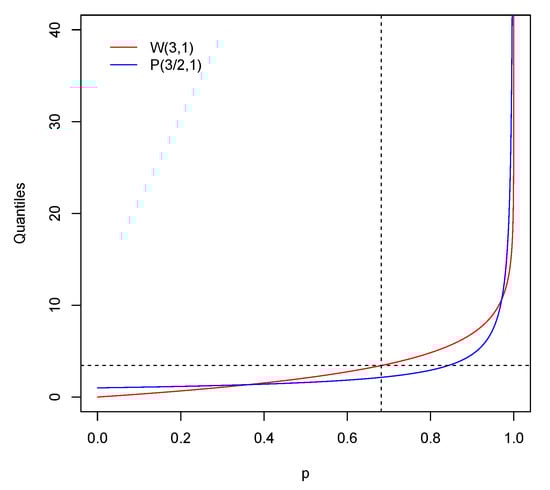
and $X{\nleqq }_{\mathrm{tcx}\left(x_0\right)}Y$. A similar reasoning shows that, in general, $X{\le }_{tcx\left(x_0\right)}Y$ does not imply $X{\le }_{p_0-\mathrm{tvar}}Y$ for $p_0<F\left(x_0\right)$. Figure 2 illustrates this situation for $X\sim W(3,1)$ and $Y\sim P(3/2,1)$, where X is Weibull and Y Pareto with distribution functions F and G, respectively. Recall that if $X\sim W(\alpha ,\beta )$ then

$$F^{-1}\left(p\right)=\alpha {\left(-log(1-p)\right)}^{1/\beta },$$

for $p\in (0,1)$. Note that $\mathrm{E}\left[X\right]=\mathrm{E}\left[Y\right]$. It can be checked that $X{\le }_{p_0-\mathrm{tvar}}Y$ with $p_0=0.68147$ (vertical line in Figure 2) and $X{\le }_{\mathrm{tcx}\left(F^{-1}\left(p_0\right)\right)}Y$ with $F^{-1}\left(p_0\right)=3.43711$ (horizontal line). However, since $G^{-1}\left(p_0\right)<F^{-1}\left(p_0\right)$ and (14) holds, $X{\nleqq }_{\mathrm{tcx}\left(x_0\right)}Y$ for any $x_0<F^{-1}\left(p_0\right)$.

Figure 2. Quantile functions for $X\sim W(3,1)$ and $Y\sim P(3/2,1)$.

Now consider two general random variables (not necessarily with the same mean). The following result connects the $p_0$-tail value at risk order and the stochastic order defined by (13).

Proposition 4.

Let X and Y be two random variables with distribution functions F and G, respectively.

(i) 

If $X{\le }_{p_0-\mathrm{tvar}}Y$, then ${\int }_x^{+\infty }\overline{F}\left(t\right)dt\le {\int }_x^{+\infty }\overline{G}\left(t\right)dt$, for all $x\ge F^{-1}\left(p_0\right)$.

(ii) 

If ${\int }_x^{+\infty }\overline{F}\left(t\right)dt\le {\int }_x^{+\infty }\overline{G}\left(t\right)dt$, for all $x\ge x_0$, then $X{\le }_{G\left(x_0\right)-tvar}Y$.

Proof. 

We prove (i) (the proof of (ii) is similar). Assume $X{\le }_{p_0-\mathrm{tvar}}Y$. From (7) we know that

$$(1-p)F^{-1}\left(p\right)+{\int }_{F^{-1}\left(p\right)}^{+\infty }\overline{F}\left(t\right)dt\le (1-p)G^{-1}\left(p\right)+{\int }_{G^{-1}\left(p\right)}^{+\infty }\overline{G}\left(t\right)dt,\mathrm{for}\mathrm{all}p\ge p_0.$$

(17)

Fixed $p\ge p_0$, the function

$$g_p\left(x\right)=(1-p)x+{\int }_x^{+\infty }\overline{G}\left(t\right)dt,\mathrm{for}\mathrm{all}x\in \mathbb{R},$$

reachs its minimum at $G^{-1}\left(p\right)$ (see Theorem 3.2 in Dhaene et al. [18]). From this fact and (17) it follows that

$$(1-p)F^{-1}\left(p\right)+{\int }_{F^{-1}\left(p\right)}^{+\infty }\overline{F}\left(t\right)dt\le (1-p)F^{-1}\left(p\right)+{\int }_{F^{-1}\left(p\right)}^{+\infty }\overline{G}\left(t\right)dt,\mathrm{for}\mathrm{all}p\ge p_0,$$

or, equivalently,

$${\int }_x^{+\infty }\overline{F}\left(t\right)dt\le {\int }_x^{+\infty }\overline{G}\left(t\right)dt,\mathrm{for}\mathrm{all}x\ge F^{-1}\left(x_0\right),$$

(18)

which concludes the proof. □

Corollary 1.

Let X and Y be two random variables with distribution functions F and G, respectively, and $p_0\in \left(0,1\right)$ such that $F^{-1}\left(p_0\right)\le G^{-1}\left(p_0\right)$. Then, $X{\le }_{p_0-tvar}Y$ if, and only if, one of the following equivalent conditions holds:

(i) 

$E\left[{\left(X-x\right)}_{+}\right]\le E\left[{\left(Y-x\right)}_{+}\right]$, for all $x\ge F^{-1}\left(p_0\right)$.

(ii) 

${\int }_x^{+\infty }\overline{F}\left(t\right)dt\le {\int }_x^{+\infty }\overline{G}\left(t\right)dt$, for all $x\ge F^{-1}\left(p_0\right)$.

Proof. 

Clearly, (i) and (ii) are equivalent. From $F^{-1}\left(p_0\right)\le G^{-1}\left(p_0\right)$ and (ii) we have

$${\int }_x^{+\infty }\overline{F}\left(t\right)dt\le {\int }_x^{+\infty }\overline{G}\left(t\right)dt,\forall x\ge G^{-1}\left(p_0\right).$$

Using Proposition 4(ii) it follows that $X{\le }_{p_0-\mathrm{tvar}}Y$. Conversely, if $X{\le }_{p_0-\mathrm{tvar}}Y$, (ii) follows from Proposition 4(i). □

The following result shows that two random variables, in which distribution functions cross a finite number of times, are ordered in the $p_0$-tail value at risk order for some $p_0\in (0,1)$. The proof is straightforward and it is omitted.

Theorem 1.

Let X and Y be two random variables with distribution functions F and G, respectively. If $S^{-}(G^{-1}-F^{-1})$ is finite, nonzero and the last sign change occurs from − to +, then $X{\le }_{p_n-\mathrm{tvar}}Y$, where $p_n$ denotes the last crossing point.

A random variable X is said to be smaller than Y in the univariate dispersive ordering (denoted by $X{\le }_{disp}Y$) if $F^{-1}\left(q\right)-F^{-1}\left(p\right)\le G^{-1}\left(q\right)-G^{-1}\left(p\right)$ for all $0<p\le q<1$. It is well-known (see Theorem 2.6.7 in Belzunce et al. [7]) that if $X{\le }_{disp}Y$ and $E\left[X\right]>E\left[Y\right]$ (which, in particular, implies that $X{\nleqq }_{icx}Y$ ), then $S^{-}(G^{-1}-F^{-1})=1$. This observation, together with Theorem 1, allows to find many parametric distributions such that $X{\le }_{p_0-\mathrm{tvar}}Y$ for some $p_0>0$ and $X{\nleqq }_{icx}Y$. Next, we provide some examples.

Example 1.

The following examples follow from Theorem 1 using results that are well-known for the dispersive order. Note that $X{\nleqq }_{icx}Y$.

(i) 

Let $X\sim N({\mu }_1,{\sigma }_1)$ and $Y\sim N({\mu }_2,{\sigma }_2)$ be two normal random variables such that ${\mu }_1>{\mu }_2$ and ${\sigma }_1<{\sigma }_2$. Then, $X{\le }_{p_0-\mathrm{tvar}}Y$, where $p_0=F_Z\left(\frac{{\mu }_1-{\mu }_2}{{\sigma }_2-{\sigma }_1}\right)$ and $Z\sim N(0,1)$.

(ii) 

Let $X\sim \mathrm{Logistic}({\mu }_1,{\sigma }_1)$ and $Y\sim \mathrm{Logistic}({\mu }_2,{\sigma }_2)$ be two logistic random variables such that ${\mu }_1>{\mu }_2$ and ${\sigma }_1<{\sigma }_2$. Then, $X{\le }_{p_0-\mathrm{tvar}}Y$, where $p_0=F_Z\left(\frac{{\mu }_1-{\mu }_2}{{\sigma }_2-{\sigma }_1}\right)$ and $Z\sim \mathrm{Logistic}(0,1)$.

(iii) 

Let $X\sim W({\lambda }_1,k_1)$ and $Y\sim W({\lambda }_2,k_2)$ be two Weibull random variables such that $\mathrm{E}\left[X\right]>\mathrm{E}\left[Y\right]$ and $k_2<k_1$. Then, $X{\le }_{p_0-\mathrm{tvar}}Y$, where $p_0=F_Z\left(a_0^{b_0}\right)$, $a_0={\lambda }_1/{\lambda }_2$, $b_0=k_1{k}_2/(k_1-k_2)$ and $Z\sim W(1,1)$.

(iv) 

Let $X\sim P(a_1,k_1)$ and $P\sim P(a_2,k_2)$ be two Pareto random variables such that $\mathrm{E}\left[X\right]>\mathrm{E}\left[Y\right]$ and $k_2<k_1$. Then, $X{\le }_{p_0-\mathrm{tvar}}Y$, where $p_0=F_Z\left(a_0^{b_0}\right)$, $a_0=a_1/a_2$, $b_0=k_1{k}_2/(k_1-k_2)$ and $Z\sim P(1,1)$.

Remark 3.

From Proposition 2 it is apparent that (i) and (ii) in Example 1 are also valid for the log-normal and log-logistic distribution families, respectively.

Remark 4.

The tail value at risk is a special case of distortion risk measure. Recall that a distortion function is a continuous, and nondecreasing function $h:[0,1]\to [0,1]$ such that $h\left(0\right)=0$ and $h\left(1\right)=1$. Given a random variable X with finite mean, the distorted random variable $X_h$ induced by h has a tail function given by

$${\overline{F}}_h\left(x\right)=h\left(\overline{F}\left(x\right)\right),$$

for all x in the support of X. It is known that given two random variables X and Y such that $X{\le }_{icx}Y$ and a concave distortion h, entonces $X_h{\le }_{icx}{Y}_h$ (see Theorem 13 in Sordo et al. [19]). It is straightforward to show (although the proof is notationally cumbersome, so we omit it) that if $X{\le }_{p_0-\mathrm{tvar}}Y$ for $p_0\in (0,1)$ and h is a concave distortion function, then $X_h{\le }_{q_0-\mathrm{tvar}}{Y}_h$ where $q_0=G_{Y_h}\left(F^{-1}\left(p_0\right)\right)$.

Before ending this section, we emphasize that, given $p_0\in (0,1)$, the order ${\le }_{p_0-tvar}$ is a pure tail order in the sense of Rojo [12]. This is shown in the following result, which shows that if $X{\le }_{p_0-tvar}Y$, then the density function $f\left(x\right)$ of X decreases faster than the density function $g\left(x\right)$ of Y.

Proposition 5.

Let X and Y be two random variables with distribution functions F and G and density functions f and g, respectively. Let $p_0\in (0,1)$. Then

$$X{\le }_{p_0-tvar}Yimplies\underset{x\to +\infty }{lim}\frac{f\left(x\right)}{g\left(x\right)}\le 1.$$

Proof. 

Just applying the L’Hôpital’s rule and using Proposition 4(i), we see that

$$\underset{x\to +\infty }{lim}\frac{f\left(x\right)}{g\left(x\right)}=\underset{x\to +\infty }{lim}\frac{{\int }_x^{+\infty }\overline{F}\left(t\right)}{{\int }_x^{+\infty }\overline{G}\left(t\right)}\le 1.$$

 □

3. A Real Data Example

In this section, we provide a financial application with a real dataset, involving two random variables of −log returns (recall that if $p_t$ denotes the price of an asset at day t, the corresponding −log return is defined by $r_t=-log(p_t/p_{t-1})$). Data are of public access and can be obtained from the Yahoo! Finance site. In order to eliminate the time dependent effect, data are related to the weekly close of trading.

We consider two national stock market indexes: the Mexican $S\&P/BMV$ IPC, denoted by MXX, that measures the performance of the largest and most liquid stocks listed on the Mexican Stock Exchange, and the Hang Seng Index, denoted by HSI, which is the main indicator of the performance of the 50 largest companies of the Hong Kong Stock Exchange. For each index, we have obtained samples of size $n=104$ corresponding to the weekly closings from 1st February 2016 until 31st January 2018. Let us denote by $R^{MXX}$ and $R^{HSI}$ the −log returns of MXX and HSI, respectively. We will obtain empirical evidence to conclude that $R^{MXX}{\nleqq }_{icx}{R}^{HSI}$ but there exists $p_0\in (0,1)$ such that $R^{MXX}{\le }_{p_0-\mathrm{tvar}}{R}^{HSI}$.

Before testing the orderings we test the randomness by a classic runs test to $R^{MXX}$ and $R^{HSI}$ and we obtain the p-values $0.237$ and $0.1149$, respectively. At this point, we plot in Figure 3 the empirical probability distributions of $R^{MXX}$ and $R^{HSI}$.

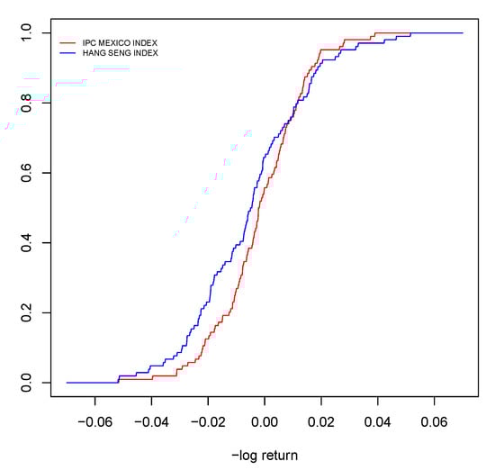
Figure 3. The empirical distribution functions of $R^{MXX}$ and $R^{HSI}$.

From Theorem 1 it is apparent that Figure 3 shows reasonable empirical evidence that $R^{MXX}{\le }_{p_0-\mathrm{tvar}}{R}^{HSI}$ for a certain value $p_0\in (0,1)$. In order to see that $R^{MXX}{\nleqq }_{icx}{R}^{HSI}$ we just need to check the expectations. For such a purpose, we first test the symmetry by performing the M, $CM$ and $MMG$ tests described in the lawstat R package. The minimum p-value of the three tests is greater than $0.05$, therefore, we cannot reject the hypothesis that both distributions, $R^{MXX}$ and $R^{HSI}$, are symmetric. Next we compare the medians by a classical Wilcoxon signed-rank test for paired samples. We obtain that the median of $R^{MXX}$ is greater than the corresponding of $R^{HSI}$, p-value$=0.01$. Therefore, since data are assumed to be symmetric, we conclude that $E\left[R^{MXX}\right]>E\left[R^{HSI}\right]$, which implies that $R^{MXX}{\nleqq }_{icx}{R}^{HSI}$.

The previous non-parametric study suggests to fit a distribution function to $R^{HSI}$ greater than $R^{MXX}$ in terms of ${\le }_{p_0-\mathrm{tvar}}$ order (with bigger tail risk). Two classical distributions for log returns are the normal and logistic distributions, where the latter better reflects an excess of kurtosis. Table 1 summarizes the p-values of the classical K-S goodness of fit test for both distribution families and Figure 4 provides the histograms of the log returns together with normal and logistic density estimates using the maximum likelihood estimates (MLE) for the location and scale parameters given in Table 2.

Table 1. The p-values for fitting normal and logistic distributions.

	K-S Goodness of Fit Test (p-Value)
Index	Normal	Logistic
MXX	$0.0512$	$0.0347$
HSI	$0.0525$	$0.0557$

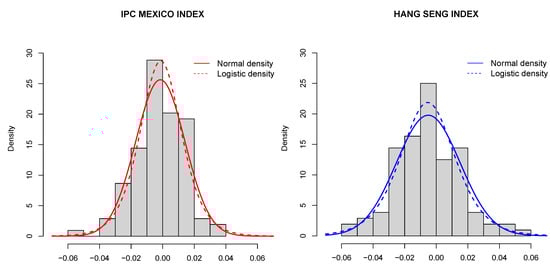
Figure 4. Histograms of the log returns with a normal density estimate (solid line) and a logistic density estimate (dashed line) superimposed. The left-hand panel corresponds to $R^{MMX}$ and right-hand panel corresponds to $R^{HSI}$.

Table 2. The maximum likelihood estimates (MLE) for normal and logistic distributions.

	Normal		Logistic
Index	$\mathit{\mu }$	$\mathit{\sigma }$	$\mathit{\mu }$	$\mathit{\sigma }$
MXX	$-0.001486327$	$0.01556418$	$-0.001226663$	$0.008706823$
HSI	$-0.005058756$	$0.02017290$	$-0.005402021$	$0.011434130$

Although Table 1 suggests than normal distributions fit better than logistics, both can be appropriate. From Example 1 there is enough evidence to assume that $R^{MXX}{\le }_{p_0-\mathrm{tvar}}{R}^{HSI}$ and the crossing point can be computed from a parametric point of view. In conclusion, a decision maker concerned by the tail value at risk for large values of p will evaluate $R^{MXX}$ as less dangerous than $R^{HSI}$ despite $\mathrm{E}\left[R^{MXX}\right]>\mathrm{E}\left[R^{HSI}\right]$ and $R^{MXX}{\nleqq }_{icx}{R}^{HSI}$.

4. Conclusions

In this paper, we have introduced a family of stochastic orders indexed by confidence levels $p_0\in (0,1)$, which are useful when we are concerned with right-tail risks. Once $p_0$ is fixed to suit our preferences, we say that X is less risky than Y if the tail value at risk of X is smaller than the tail value at risk of Y for any confidence levels p such that $p>p_0.$ We have studied the properties of this family of orders as well as its relationships with other stochastic orders, in particular with the tail convex order introduced by Cheung and Vandulfel [8]. We have illustrated the results with a real financial dataset involving log returns.

References

- Wang, S. An actuarial index of the right-tail risk. N. Am. Actuar. J. 1998, 2, 88–101. [Google Scholar] [CrossRef]
- Guégan, D.; Hassani, B.K. Risk Measurement; Springer: Cham, Switzerland, 2019. [Google Scholar]
- Zhelonkin, M.; Chavez-Demoulin, V. A note on the statistical robustness of risk measures. J. Oper. Risk 2017, 12, 47–68. [Google Scholar] [CrossRef]
- Ahmadi-Javid, A. Entropic value-at-risk: A new coherent risk measure. Eur. J. Oper. Res. 2019, 279, 225–241. [Google Scholar] [CrossRef]
- Sordo, M.A.; Ramos, H.M. Characterization of stochastic orderings by L-functionals. Stat. Pap. 2007, 48, 249–263. [Google Scholar] [CrossRef]
- Shaked, M.; Shanthikumar, J.G. Stochastic Orders; Springer Series in Statistics; Springer: New York, NY, USA, 2007. [Google Scholar]
- Belzunce, F.; Martínez-Riquelme, C.; Mulero, J. An Introduction to Stochastic Orders; Academic Press, Elsevier Ltd.: London, UK, 2016. [Google Scholar]
- Cheung, K.C.; Vanduffel, S. Bounds for sums of random variables when the marginal distributions and the variance of the sum are given. Scand. Actuar. J. 2013, 2, 103–118. [Google Scholar] [CrossRef]
- Sordo, M.A.; de Souza, M.C.; Suárez-LLorens, A. A new variability order based on tail-heaviness. Statistics 2015, 49, 1042–1061. [Google Scholar] [CrossRef]
- Mulero, J.; Sordo, M.A.; de Souza, M.C.; Suárez-Llorens, A. Two stochastic dominance criteria based on tail comparisons. Appl. Stoch. Model. Bus. Ind. 2017, 33, 575–589. [Google Scholar] [CrossRef]
- Belzunce, F.; Franco-Pereira, A.M.; Mulero, J. New stochastic comparisons based on tail value at risk measures. Commun. Stat. Theory Methods 2020. [Google Scholar] [CrossRef]
- Rojo, J. A pure tail ordering based on the ratio of the quantile functions. Ann. Stat. 1992, 20, 570–579. [Google Scholar] [CrossRef]
- Van der Vaart, A.W. Asymptotic Statistics; Cambridge University Press: Cambridge, UK, 1998. [Google Scholar]
- Müller, A. Orderings of Risks: A comparative study via stop-loss transforms. Insur. Math. Econ. 1996, 17, 215–222. [Google Scholar] [CrossRef]
- Barlow, R.E.; Proschan, F. Statistical Theory of Reliability and Life Testing; Holt, Rinehart and Winston, Inc.: New York, NY, USA, 1975. [Google Scholar]
- Zygmund, A. Trigonometric Series; Cambridge University Press: Cambridge, UK, 1959. [Google Scholar]
- Cheung, K.C.; Lo, A. Characterizations of counter-monotonicity and upper comonotonicity by (tail) convex order. Insur. Math. Econ. 2013, 53, 334–342. [Google Scholar] [CrossRef]
- Dhaene, J.; Vanduffel, S.; Goovaerts, M.; Kaas, R.; Tang, Q.; Vyncke, D. Risk measures and comonotonicity: A review. Stoch. Model. 2006, 22, 573–606. [Google Scholar] [CrossRef]
- Sordo, M.A.; Suárez-Llorens, A.; Bello, A.J. Comparisons of conditional distributions in portfolios of dependent risks. Insur. Math. Econ. 2015, 61, 62–69. [Google Scholar] [CrossRef]
© 2020 by the authors. Licensee MDPI, Basel, Switzerland. This article is an open access article distributed under the terms and conditions of the Creative Commons Attribution (CC BY) license (http://creativecommons.org/licenses/by/4.0/).