On Derivative Free Multiple-Root Finders with Optimal Fourth Order Convergence

Abstract

A number of optimal order multiple root techniques that require derivative evaluations in the formulas have been proposed in literature. However, derivative-free optimal techniques for multiple roots are seldom obtained. By considering this factor as motivational, here we present a class of optimal fourth order methods for computing multiple roots without using derivatives in the iteration. The iterative formula consists of two steps in which the first step is a well-known Traub–Steffensen scheme whereas second step is a Traub–Steffensen-like scheme. The Methodology is based on two steps of which the first is Traub–Steffensen iteration and the second is Traub–Steffensen-like iteration. Effectiveness is validated on different problems that shows the robust convergent behavior of the proposed methods. It has been proven that the new derivative-free methods are good competitors to their existing counterparts that need derivative information.

1. Introduction

Finding root of a nonlinear equation $\psi \left(u\right)=0$ is a very important and interesting problem in many branches of science and engineering. In this work, we examine derivative-free numerical methods to find a multiple root (say, $\alpha$) with multiplicity $\mu$ of the equation $\psi \left(u\right)=0$ that means ${\psi }^{\left(j\right)}\left(\alpha \right)=0,j=0,1,2,...,\mu -1$ and ${\psi }^{\left(\mu \right)}\left(\alpha \right)\ne 0$. Newton’s method [1] is the most widely used basic method for finding multiple roots, which is given by

$$u_{k+1}=u_k-\mu \frac{\psi \left(u_k\right)}{{\psi }^{\prime }\left(u_k\right)},k=0,1,2,\dots ,\mu =2,3,4,\dots .$$

(1)

A number of modified methods, with or without the base of Newton’s method, have been elaborated and analyzed in literature, see [2,3,4,5,6,7,8,9,10,11,12,13,14]. These methods use derivatives of either first order or both first and second order in the iterative scheme. Contrary to this, higher order methods without derivatives to calculate multiple roots are yet to be examined. These methods are very useful in the problems where the derivative ${\psi }^{\prime }$ is cumbersome to evaluate or is costly to compute. The derivative-free counterpart of classical Newton method (1) is the Traub–Steffensen method [15]. The method uses the approximation

$${\psi }^{\prime }\left(u_k\right)\simeq \frac{\psi (u_k+\beta \psi \left(u_k\right))-\psi \left(u_k\right)}{\beta \psi \left(u_k\right)},\beta \in \mathbb{R}-\left\{0\right\},$$

or

$${\psi }^{\prime }\left(u_k\right)\simeq \psi [v_k,u_k],$$

for the derivative ${\psi }^{\prime }$ in the Newton method (1). Here, $v_k=u_k+\beta \psi \left(u_k\right)$ and $\psi [v_k,u_k]=\frac{\psi \left(v_k\right)-\psi \left(u_k\right)}{v_k-u_k}$ is a first order divided difference. Thereby, the method (1) takes the form of the Traub–Steffensen scheme defined as

$$u_{k+1}=u_k-\mu \frac{\psi \left(u_k\right)}{\psi [v_k,u_k]}.$$

(2)

The Traub–Steffensen method (2) is a prominent improvement of the Newton method because it maintains the quadratic convergence without adding any derivative.

Unlike Newton-like methods, the Traub–Steffensen-like methods are difficult to construct. Recently, a family of two-step Traub–Steffensen-like methods with fourth order convergence has been proposed in [16]. In terms of computational cost, the methods of [16] use three function evaluations per iteration and thus possess optimal fourth order convergence according to Kung–Traub conjecture (see [17]). This hypothesis states that multi-point methods without memory requiring m functional evaluations can attain the convergence order $2^{m-1}$ called optimal order. Such methods are usually known as optimal methods. Our aim in this work is to develop derivative-free multiple root methods of good computational efficiency, which is to say, the methods of higher convergence order with the amount of computational work as small as we please. Consequently, we introduce a class of Traub–Steffensen-like derivative-free fourth order methods that require three new pieces of information of the function $\psi$ and therefore have optimal fourth order convergence according to Kung–Traub conjecture. The iterative formula consists of two steps with Traub–Steffensen iteration (2) in the first step, whereas there is Traub–Steffensen-like iteration in the second step. Performance is tested numerically on many problems of different kinds. Moreover, comparison of performance with existing modified Newton-like methods verifies the robust and efficient nature of the proposed methods.

We summarize the contents of paper. In Section 2, the scheme of fourth order iteration is formulated and convergence order is studied separately for different cases. The main result, showing the unification of different cases, is studied in Section 3. Section 4 contains the basins of attractors drawn to assess the convergence domains of new methods. In Section 5, numerical experiments are performed on different problems to demonstrate accuracy and efficiency of the methods. Concluding remarks about the work are reported in Section 6.

2. Development of a Novel Scheme

Researchers have used different approaches to develop higher order iterative methods for solving nonlinear equations. Some of them are: Interpolation approach, Sampling approach, Composition approach, Geometrical approach, Adomian approach, and Weight-function approach. Of these, the Weight-function approach has been most popular in recent times; see, for example, Refs. [10,13,14,18,19] and references therein. Using this approach, we consider the following two-step iterative scheme for finding multiple root with multiplicity $\mu \ge 2$:

$$\begin{array}{cc}\hfill z_k=& u_k-\mu \frac{\psi \left(u_k\right)}{\psi [v_k,u_k]},\hfill \\ \hfill u_{k+1}=& z_k-G\left(h\right)\left(1+\frac{1}{y_k}\right)\frac{\psi \left(u_k\right)}{\psi [v_k,u_k]},\hfill \end{array}$$

(3)

where $h=\frac{x_k}{1+x_k}$, $x_k=\sqrt[\mu ]{\frac{\psi \left(z_k\right)}{\psi \left(u_k\right)}}$, $y_k=\sqrt[\mu ]{\frac{\psi \left(v_k\right)}{\psi \left(u_k\right)}}$ and $G:\mathbb{C}\to \mathbb{C}$ is analytic in the neighborhood of zero. This iterative scheme is weighted by the factors $G\left(h\right)$ and $\left(1+\frac{1}{y_k}\right)$, hence the name weight-factor or weight-function technique.

Note that $x_k$ and $y_k$ are one-to-$\mu$ multi-valued functions, so we consider their principal analytic branches [18]. Hence, it is convenient to treat them as the principal root. For example, let us consider the case of $x_k$. The principal root is given by $x_k=\exp \left[\frac{1}{\mu }\mathrm{Log}\left(\frac{\psi \left(z_k\right)}{\psi \left(u_k\right)}\right)\right]$, with $\mathrm{Log}\left(\frac{\psi \left(z_k\right)}{\psi \left(u_k\right)}\right)=\mathrm{Log}\left|\frac{\psi \left(z_k\right)}{\psi \left(u_k\right)}\right|+i\mathrm{Arg}\left(\frac{\psi \left(z_k\right)}{\psi \left(u_k\right)}\right)$ for $-\pi <\mathrm{Arg}\left(\frac{\psi \left(z_k\right)}{\psi \left(u_k\right)}\right)\le \pi$; this convention of $\mathrm{Arg}\left(p\right)$ for $p\in \mathbb{C}$ agrees with that of $\mathrm{Log}\left[p\right]$ command of Mathematica [20] to be employed later in the sections of basins of attraction and numerical experiments. Similarly, we treat for $y_k$.

In the sequel, we prove fourth order of convergence of the proposed iterative scheme (3). For simplicity, the results are obtained separately for the cases depending upon the multiplicity $\mu$. Firstly, we consider the case $\mu =2$.

Theorem 1. 

Assume that $u=\alpha$ is a zero with multiplicity $\mu =2$ of the function $\psi \left(u\right)$, where $\psi :\mathbb{C}\to \mathbb{C}$ is sufficiently differentiable in a domain containing α. Suppose that the initial point $u_0$ is closer to α; then, the order of convergence of the scheme (3) is at least four, provided that the weight-function $G\left(h\right)$ satisfies the conditions $G\left(0\right)=0$, $G^{\prime }\left(0\right)=1$, $G^{″}\left(0\right)=6$ and $|G^{‴}\left(0\right)|<\infty$.

Proof. 

Assume that ${\epsilon }_k=u_k-\alpha$ is the error at the k-th stage. Expanding $\psi \left(u_k\right)$ about $\alpha$ using the Taylor series keeping in mind that $\psi \left(\alpha \right)=0$, ${\psi }^{\prime }\left(\alpha \right)=0$ and ${\psi }^{\left(2\right)}\left(\alpha \right)\ne 0,$, we have that

$$\psi \left(u_k\right)=\frac{{\psi }^{\left(2\right)}\left(\alpha \right)}{2!}{\epsilon }_k^2\left(1+A_1{\epsilon }_k+A_2{\epsilon }_k^2+A_3{\epsilon }_k^3+A_4{\epsilon }_k^4+\cdots \right),$$

(4)

where $A_m=\frac{2!}{(2+m)!}\frac{{\psi }^{(2+m)}\left(\alpha \right)}{{\psi }^{\left(2\right)}\left(\alpha \right)}$ for $m\in \mathbb{N}$.

Similarly, Taylor series expansion of $\psi \left(v_k\right)$ is

$$\psi \left(v_k\right)=\frac{{\psi }^{\left(2\right)}\left(\alpha \right)}{2!}{\epsilon }_{v_k}^2\left(1+A_1{\epsilon }_{v_k}+A_2{\epsilon }_{v_k}^2+A_3{\epsilon }_{v_k}^3+A_4{\epsilon }_{v_k}^4+\cdots \right),$$

(5)

where ${\epsilon }_{v_k}=v_k-\alpha ={\epsilon }_k+\frac{\beta {\psi }^{\left(2\right)}\left(\alpha \right)}{2!}{\epsilon }_k^2\left(1+A_1{\epsilon }_k+A_2{\epsilon }_k^2+A_3{\epsilon }_k^3+A_4{\epsilon }_k^4+\cdots \right).$

By using (4) and (5) in the first step of (3), we obtain

$$\begin{array}{lll}{\epsilon }_{z_k}& =& z_k-\alpha \\ & =& \frac{1}{2}\left(\frac{\beta {\psi }^{\left(2\right)}\left(\alpha \right)}{2}+A_1\right){\epsilon }_k^2-\frac{1}{16}\left({\left(\beta {\psi }^{\left(2\right)}\left(\alpha \right)\right)}^2-8\beta {\psi }^{\left(2\right)}\left(\alpha \right)A_1+12A_1^2-16A_2\right){\epsilon }_k^3+\frac{1}{64}({\left(\beta {\psi }^{\left(2\right)}\left(\alpha \right)\right)}^3\\ & & -20\beta {\psi }^{\left(2\right)}\left(\alpha \right)A_1^2+72A_1^3+64\beta {\psi }^{\left(2\right)}\left(\alpha \right)A_2-10A_1\left({\left(\beta {\psi }^{\left(2\right)}\left(\alpha \right)\right)}^2+16A_2\right)+96A_3){\epsilon }_k^4+O\left({\epsilon }_k^5\right).\end{array}$$

(6)

In addition, we have that

$$\psi \left(z_k\right)=\frac{{\psi }^{\left(2\right)}\left(\alpha \right)}{2!}{\epsilon }_{z_k}^2\left(1+A_1{\epsilon }_{z_k}+A_2{\epsilon }_{z_k}^2+\cdots \right).$$

(7)

Using (4), (5) and (7), we further obtain

$$\begin{array}{ll}{x}_k=& \frac{1}{2}\left(\frac{\beta {\psi }^{\left(2\right)}\left(\alpha \right)}{2}+A_1\right){\epsilon }_k-\frac{1}{16}\left({\left(\beta {\psi }^{\left(2\right)}\left(\alpha \right)\right)}^2-6\beta {\psi }^{\left(2\right)}\left(\alpha \right)A_1+16(A_1^2-A_2)\right){\epsilon }_k^2+\frac{1}{64}({\left(\beta {\psi }^{\left(2\right)}\left(\alpha \right)\right)}^3\\ & -22\beta {\psi }^{\left(2\right)}\left(\alpha \right)A_1^2+4\left(29A_1^3+14\beta {\psi }^{\left(2\right)}\left(\alpha \right)A_2\right)-2A_1\left(3{\left(\beta {\psi }^{\left(2\right)}\left(\alpha \right)\right)}^2+104A_2\right)+96A_3){\epsilon }_k^3\\ & +\frac{1}{256}(212\beta {\psi }^{\left(2\right)}\left(\alpha \right)A_1^3-800A_1^4+2A_1^2(-7{\left(\beta {\psi }^{\left(2\right)}\left(\alpha \right)\right)}^2+1040A_2)+2A_1(3{\left(\beta {\psi }^{\left(2\right)}\left(\alpha \right)\right)}^3-232\beta {\psi }^{\left(2\right)}\left(\alpha \right)A_2\\ & -576A_3)-({\left(\beta {\psi }^{\left(2\right)}\left(\alpha \right)\right)}^4+8\beta {\psi }^{\left(2\right)}\left(\alpha \right)A_2+640A_2^2-416\beta {\psi }^{\left(2\right)}\left(\alpha \right)A_3-512A_4)){\epsilon }_k^4+O\left({\epsilon }_k^5\right)\end{array}$$

(8)

and

$$\begin{array}{ll}{y}_k=& 1+\frac{\beta {\psi }^{\left(2\right)}\left(\alpha \right)}{2}{\epsilon }_k(1+\frac{3}{2}{A}_1{\epsilon }_k+\frac{1}{4}\left(\beta {\psi }^{\left(2\right)}\left(\alpha \right)A_1+8A_2\right){\epsilon }_k^2+\frac{1}{16}\left(3\beta {\psi }^{\left(2\right)}\left(\alpha \right)A_1^2+12\beta {\psi }^{\left(2\right)}\left(\alpha \right)A_2+40A_3\right){\epsilon }_k^3\\ & +O\left({\epsilon }_k^4\right)).\end{array}$$

(9)

Using (8), we have

$$\begin{array}{ll}h=& \frac{1}{2}\left(\frac{\beta {\psi }^{\left(2\right)}\left(\alpha \right)}{2}+A_1\right){\epsilon }_k-\frac{1}{8}\left({\left(\beta {\psi }^{\left(2\right)}\left(\alpha \right)\right)}^2-\beta {\psi }^{\left(2\right)}\left(\alpha \right)A_1-2(4A_2-5A_1^2)\right){\epsilon }_k^2+\frac{1}{32}(-\beta {\psi }^{\left(2\right)}\left(\alpha \right)A_1^2+94A_1^3\\ & -4A_1({\left(\beta {\psi }^{\left(2\right)}\left(\alpha \right)\right)}^2+34A_2)+2({\left(\beta {\psi }^{\left(2\right)}\left(\alpha \right)\right)}^3+6\beta {\psi }^{\left(2\right)}\left(\alpha \right)A_2+24A_3)){\epsilon }_k^3+\frac{1}{128}(54\beta {\psi }^{\left(2\right)}\left(\alpha \right)A_1^3-864A_1^4\\ & +A_1^2(1808A_2-13{\left(\beta {\psi }^{\left(2\right)}\left(\alpha \right)\right)}^2)+2A_1(6{\left(\beta {\psi }^{\left(2\right)}\left(\alpha \right)\right)}^3-68\beta {\psi }^{\left(2\right)}\left(\alpha \right)A_2-384A_3)-4({\left(\beta {\psi }^{\left(2\right)}\left(\alpha \right)\right)}^4\\ & +5{\left(\beta {\psi }^{\left(2\right)}\left(\alpha \right)\right)}^2{A}_2+112A_2^2-28\beta {\psi }^{\left(2\right)}\left(\alpha \right)A_3-64A_4\left)\right){\epsilon }_k^4+O\left({\epsilon }_k^5\right).\end{array}$$

(10)

Taylor expansion of the weight function $G\left(h\right)$ in the neighborhood of origin up to third-order terms is given by

$$G\left(h\right)\approx G\left(0\right)+h{G}^{\prime }\left(0\right)+\frac{1}{2}{h}^2{G}^{″}\left(0\right)+\frac{1}{6}{h}^2{G}^{‴}\left(0\right).$$

(11)

Using (4)–(11) in the last step of (3), we have

$$\begin{array}{cc}\hfill {\epsilon }_{k+1}=& -G\left(0\right){\epsilon }_k+\frac{1}{4}\left(\beta {\psi }^{\left(2\right)}\left(\alpha \right)(1+2G\left(0\right)-G^{\prime }\left(0\right))+2(1+G\left(0\right)-G^{\prime }\left(0\right))A_1\right){\epsilon }_k^2+\sum _{n=1}^2{\varphi }_n{\epsilon }_k^{n+2}+O\left({\epsilon }_k^5\right),\hfill \end{array}$$

(12)

where ${\varphi }_n={\varphi }_n(\beta ,A_1,A_2,A_3,G\left(0\right),G^{\prime }\left(0\right),G^{″}\left(0\right),G^{‴}\left(0\right))$, $n=1,2.$ The expressions of ${\varphi }_1$ and ${\varphi }_2$ being very lengthy have not been produced explicitly.

We can obtain at least fourth order convergence if we set coefficients of ${\epsilon }_k$, ${\epsilon }_k^2$ and ${\epsilon }_k^3$ simultaneously equal to zero. Then, some simple calculations yield

$$G\left(0\right)=0,G^{\prime }\left(0\right)=1,G^{″}\left(0\right)=6.$$

(13)

Using (13) in (12), we will obtain final error equation

$$\begin{array}{ll}{\epsilon }_{k+1}=& -\frac{1}{192}\left(\frac{\beta {\psi }^{\left(2\right)}\left(\alpha \right)}{2}+A_1\right)((G^{‴}\left(0\right)-42){\left(\beta {\psi }^{\left(2\right)}\left(\alpha \right)\right)}^2+4(G^{‴}\left(0\right)-45)\beta {\psi }^{\left(2\right)}\left(\alpha \right)A_1+4(G^{‴}\left(0\right)-63)A_1^2\\ & +48A_2){\epsilon }_k^4+O\left({\epsilon }_k^5\right).\end{array}$$

(14)

Thus, the theorem is proved. □

Next, we prove the following theorem for case $\mu =3$.

Theorem 2. 

Using assumptions of Theorem 1, the convergence order of scheme (3) for the case $\mu =3$ is at least 4, if $G\left(0\right)=0$, $G^{\prime }\left(0\right)=\frac{3}{2}$, $G^{″}\left(0\right)=9$ and $|G^{‴}\left(0\right)|<\infty$.

Proof. 

Taking into account that $\psi \left(\alpha \right)=0$, ${\psi }^{\prime }\left(\alpha \right)=0$, ${\psi }^{{}^{″}}\left(\alpha \right)=0$ and ${\psi }^{\left(3\right)}\left(\alpha \right)\ne 0$, the Taylor series development of $\psi \left(u_k\right)$ about $\alpha$ gives

$$\psi \left(u_k\right)=\frac{{\psi }^{\left(3\right)}\left(\alpha \right)}{3!}{\epsilon }_k^3\left(1+B_1{\epsilon }_k+B_2{\epsilon }_k^2+B_3{\epsilon }_k^3+B_4{\epsilon }_k^4+\cdots \right),$$

(15)

where $B_m=\frac{3!}{(3+m)!}\frac{{\psi }^{(3+m)}\left(\alpha \right)}{{\psi }^{\left(3\right)}\left(\alpha \right)}$ for $m\in \mathbb{N}$.

Expanding $\psi \left(v_k\right)$ about $\alpha$

$$\psi \left(v_k\right)=\frac{{\psi }^{\left(3\right)}\left(\alpha \right)}{3!}{\epsilon }_{v_k}^3\left(1+B_1{\epsilon }_{v_k}+B_2{\epsilon }_{v_k}^2+B_3{\epsilon }_{v_k}^3+B_4{\epsilon }_{v_k}^4+\cdots \right),$$

(16)

where ${\epsilon }_{v_k}=v_k-\alpha ={\epsilon }_k+\frac{\beta {\psi }^{\left(3\right)}\left(\alpha \right)}{3!}{\epsilon }_k^3\left(1+B_1{\epsilon }_k+B_2{\epsilon }_k^2+B_3{\epsilon }_k^3+B_4{\epsilon }_k^4+\cdots \right).$

Then, using (15) and (16) in the first step of (3), we obtain

$$\begin{array}{ll}{\epsilon }_{z_k}& =z_k-\alpha \\ \hfill & =\frac{B_1}{3}{\epsilon }_k^2+\frac{1}{18}\left(3\beta {\psi }^{\left(3\right)}\left(\alpha \right)-8B_1^2+12B_2\right){\epsilon }_k^3+\frac{1}{27}\left(16B_1^3+3B_1\left(2\beta {\psi }^{\left(3\right)}\left(\alpha \right)-13B_2\right)+27B_3\right){\epsilon }_k^4+O\left({\epsilon }_k^5\right).\end{array}$$

(17)

Expansion of $\psi \left(z_k\right)$ about $\alpha$ yields

$$\psi \left(z_k\right)=\frac{{\psi }^{\left(3\right)}\left(\alpha \right)}{3!}{\epsilon }_{z_k}^3\left(1+B_1{\epsilon }_{z_k}+B_2{\epsilon }_{z_k}^2+B_3{\epsilon }_{z_k}^3+B_4{\epsilon }_{z_k}^4+\cdots \right).$$

(18)

Then, from (15), (16), and (18), it follows that

$$\begin{array}{ll}{x}_k=& \frac{B_1}{3}{\epsilon }_k+\frac{1}{18}\left(3\beta {\psi }^{\left(3\right)}\left(\alpha \right)-10B_1^2+12B_2\right){\epsilon }_k^2+\frac{1}{54}\left(46B_1^3+3B_1\left(3{\psi }^{\left(3\right)}\left(\alpha \right)\beta -32B_2\right)+54B_3\right){\epsilon }_k^3-\frac{1}{486}(610B_1^4\\ & -B_1^2(1818B_2-27\beta {\psi }^{\left(3\right)}\left(\alpha \right))+1188B_1{B}_3+9\left({\left(\beta {\psi }^{\left(3\right)}\left(\alpha \right)\right)}^2-15\beta {\psi }^{\left(3\right)}\left(\alpha \right)B_2+72B_2^2-72B_4\right)){\epsilon }_k^4+O\left({\epsilon }_k^5\right)\end{array}$$

(19)

and

$$y_k=1+\frac{\beta {\psi }^{\left(3\right)}\left(\alpha \right)}{3!}{\epsilon }_k^2\left(1+\frac{4}{3}{B}_1{\epsilon }_k+\frac{5}{3}{B}_2{\epsilon }_k^2+\frac{1}{18}(\beta {\psi }^{\left(3\right)}\left(\alpha \right)B_1+36B_3){\epsilon }_k^3+O\left({\epsilon }_k^4\right)\right).$$

(20)

Using (19), we have

$$\begin{array}{ll}h=& \frac{B_1}{3}{\epsilon }_k+\frac{1}{6}\left(\beta {\psi }^{\left(3\right)}\left(\alpha \right)-4B_1^2+4B_2\right){\epsilon }_k^2+\frac{1}{54}\left(68B_1^3+3B_1\left(\beta {\psi }^{\left(3\right)}\left(\alpha \right)-40B_2\right)+54B_3\right){\epsilon }_k^3-\frac{1}{2916}(6792B_1^4\\ & -108B_1^2(159B_2+2\beta {\psi }^{\left(3\right)}\left(\alpha \right))+9072B_1{B}_3-27\left(-5{\left(\beta {\psi }^{\left(3\right)}\left(\alpha \right)\right)}^2+6\beta {\psi }^{\left(3\right)}\left(\alpha \right)B_2-192B_2^2+144B_4\right)){\epsilon }_k^4\\ & +O\left({\epsilon }_k^5\right).\end{array}$$

(21)

Developing weight function $G\left(h\right)$ about origin by the Taylor series expansion,

$$G\left(h\right)\approx G\left(0\right)+h{G}^{\prime }\left(0\right)+\frac{1}{2}{h}^2{G}^{″}\left(0\right)+\frac{1}{6}{h}^3{G}^{‴}\left(0\right).$$

(22)

By using (15)–(22) in the last step of (3), we have

$$\begin{array}{c}\hfill {\epsilon }_{k+1}=-\frac{2G\left(0\right)}{3}{\epsilon }_k+\frac{1}{9}(3+2G\left(0\right)-2G^{\prime }\left(0\right))B_1{\epsilon }_k^2+\sum _{n=1}^2{\phi }_n{\epsilon }_k^{n+2}+O\left({\epsilon }_k^5\right),\end{array}$$

(23)

where ${\phi }_n={\phi }_n(\beta ,B_1,B_2,B_3,G\left(0\right),G^{\prime }\left(0\right),G^{″}\left(0\right),G^{‴}\left(0\right))$, $n=1,2.$

To obtain fourth order convergence, it is sufficient to set coefficients of ${\epsilon }_k$, ${\epsilon }_k^2$, and ${\epsilon }_k^3$ simultaneously equal to zero. This process will yield

$$G\left(0\right)=0,G^{\prime }\left(0\right)=\frac{3}{2},G^{″}\left(0\right)=9.$$

(24)

Then, error equation (23) is given by

$${\epsilon }_{k+1}=-\frac{B_1}{972}\left(27\beta {\psi }^{\left(3\right)}\left(\alpha \right)+4(G^{‴}\left(0\right)-99)B_1^2+108B_2\right){\epsilon }_k^4+O\left({\epsilon }_k^5\right).$$

(25)

Hence, the result is proved. □

Remark 1. 

We can observe from the above results that the number of conditions on $G\left(h\right)$ is 3 corresponding to the cases $\mu =2,3$ to attain the fourth order convergence of the method (3). These cases also satisfy common conditions: $G\left(0\right)=0$, $G^{\prime }\left(0\right)=\frac{\mu }{2}$, $G^{″}\left(0\right)=3\mu$. Their error equations also contain the term involving the parameter β. However, for the cases $\mu \ge 4$, it has been seen that the error equation in each such case does not contain β term. We shall prove this fact in the next section.

3. Main Result

We shall prove the convergence order of scheme (3) for the multiplicity $\mu \ge 4$ by the following theorem:

Theorem 3. 

Using assumptions of Theorem 1, the convergence order of scheme (3) for $\mu \ge 4$ is at least four, provided that $G\left(0\right)=0$, $G^{\prime }\left(0\right)=\frac{\mu }{2}$, $G^{″}\left(0\right)=3\mu$ and $|G^{‴}\left(0\right)|<\infty$. Moreover, error in the scheme is given by

$${\epsilon }_{k+1}=\frac{1}{6{\mu }^4}\left((3\mu (19+\mu )-2G^{‴}\left(0\right))F_1^3-6{\mu }^2{F}_1{F}_2\right){\epsilon }_k^4+O\left({\epsilon }_k^5\right),$$

where $F_m=\frac{\mu !}{(\mu +m)!}\frac{{\psi }^{(\mu +m)}\left(\alpha \right)}{{\psi }^{\left(\mu \right)}\left(\alpha \right)}$ for $m\in \mathbb{N}$.

Proof. 

Taking into account that ${\psi }^{\left(i\right)}\left(\alpha \right)=0,i=0,1,2,...,\mu -1$ and ${\psi }^{\left(\mu \right)}\left(\alpha \right)\ne 0$, then Taylor series expansion of $\psi \left(u_k\right)$ about $\alpha$ is

$$\psi \left(u_k\right)=\frac{{\psi }^{\left(\mu \right)}\left(\alpha \right)}{\mu !}{\epsilon }_k^{\mu }\left(1+F_1{\epsilon }_k+F_2{\epsilon }_k^2+F_3{\epsilon }_k^3+F_4{\epsilon }_k^4+\cdots \right).$$

(26)

Taylor expansion of $\psi \left(v_k\right)$ about $\alpha$ yields

$$\psi \left(v_k\right)=\frac{{\psi }^{\left(\mu \right)}\left(\alpha \right)}{\mu !}{\epsilon }_{v_k}^{\mu }\left(1+F_1{\epsilon }_{v_k}+F_2{\epsilon }_{v_k}^2+F_3{\epsilon }_{v_k}^3+F_4{\epsilon }_{v_k}^4+\cdots \right),$$

(27)

where ${\epsilon }_{v_k}=v_k-\alpha ={\epsilon }_k+\frac{\beta {\psi }^{\left(\mu \right)}\left(\alpha \right)}{\mu !}{\epsilon }_k^{\mu }\left(1+F_1{\epsilon }_k+F_2{\epsilon }_k^2+F_3{\epsilon }_k^3+F_4{\epsilon }_k^4+\cdots \right).$

Using (26) and (27) in the first step of (3), we obtain

$${\epsilon }_{z_k}=\left\{\begin{array}{l}\frac{F_1}{4}{\epsilon }_k^2+\frac{1}{16}\left(8F_2-5F_1^2\right){\epsilon }_k^3+\frac{1}{64}\left(4\beta {\psi }^{\left(4\right)}\left(\alpha \right)+25F_1^3-64F_1{F}_2+48F_3\right){\epsilon }_k^4+O\left({\epsilon }_k^5\right),\mathrm{if}\mu =4,\\ \frac{F_1}{\mu }{\epsilon }_k^2+\frac{1}{{\mu }^2}\left(2\mu F_2-(1+\mu )F_1^2\right){\epsilon }_k^3+\frac{1}{{\mu }^3}\left({(1+\mu )}^2{F}_1^3-\mu (4+3\mu )F_1{F}_2+3{\mu }^2{F}_3\right){\epsilon }_k^4+O\left({\epsilon }_k^5\right),\mathrm{if}\mu \ge 5,\end{array}\right.$$

(28)

where ${\epsilon }_{z_k}=z_k-\alpha .$

Expansion of $\psi \left(z_k\right)$ around $\alpha$ yields

$$\psi \left(z_k\right)=\frac{{\psi }^{\left(\mu \right)}\left(\alpha \right)}{\mu !}{\epsilon }_{z_k}^{\mu }\left(1+F_1{\epsilon }_{z_k}+F_2{\epsilon }_{z_k}^2+F_3{\epsilon }_{z_k}^3+F_4{\epsilon }_{z_k}^4+\cdots \right).$$

(29)

Using (26), (27) and (29), we have that

$$x_k=\left\{\begin{array}{l}\frac{F_1}{4}{\epsilon }_k+\frac{1}{8}\left(4F_2-3F_1^2\right){\epsilon }_k^2+\frac{1}{128}\left(8\beta {\psi }^{\left(4\right)}\left(\alpha \right)+67F_1^3-152F_1{F}_2+96F_3\right){\epsilon }_k^3+\frac{1}{768}(-543F_1^4+1740F_1^2{F}_2\\ +4F_1(11\beta {\psi }^{\left(4\right)}\left(\alpha \right)-312F_3)+96(-7F_2^2+8F_4)){\epsilon }_k^4+O\left({\epsilon }_k^5\right),\mathrm{if}\mu =4,\\ \frac{F_1}{5}{\epsilon }_k+\frac{1}{25}\left(10F_2-7F_1^2\right){\epsilon }_k^2+\frac{1}{125}\left(46F_1^3-110F_1{F}_2+75F_3\right){\epsilon }_k^3+(\frac{\beta {\psi }^{\left(5\right)}\left(\alpha \right)}{60}-\frac{294}{625}{F}_1^4+\frac{197}{125}{F}_1^2{F}_2-\frac{16}{25}{F}_2^2\\ -\frac{6}{5}{F}_1{F}_3+\frac{4}{5}{F}_4){\epsilon }_k^4+O\left({\epsilon }_k^5\right),\mathrm{if}\mu =5,\\ \frac{F_1}{\mu }{\epsilon }_k+\frac{1}{{\mu }^2}\left(2\mu F_2-(2+\mu )F_1^2\right){\epsilon }_k^2+\frac{1}{2{\mu }^3}\left((7+7\mu +2{\mu }^2)F_1^3-2\mu (7+3\mu )F_1{F}_2+6{\mu }^2{F}_3\right){\epsilon }_k^3\\ -\frac{1}{6{\mu }^4}((34+51\mu +29{\mu }^2+6{\mu }^3)F_1^4-6\mu (17+16\mu +4{\mu }^2)F_1^2{F}_2+12{\mu }^2(3+\mu )F_2^2\\ +12{\mu }^2(5+2\mu )F_1{F}_3){\epsilon }_k^4+O\left({\epsilon }_k^5\right),\mathrm{if}\mu \ge 6\end{array}\right.$$

(30)

and

$$y_k=1+\frac{\beta {\psi }^{\left(\mu \right)}\left(\alpha \right)}{\mu !}{\epsilon }_k^{\mu -1}\left(1+\frac{(\mu +1)F_1}{\mu }{\epsilon }_k+\frac{(\mu +2)F_2}{\mu }{\epsilon }_k^2+\frac{(\mu +3)F_3}{\mu }{\epsilon }_k^3+\frac{(\mu +4)F_4}{\mu }{\epsilon }_k^4+O\left({\epsilon }_k^5\right)\right).$$

(31)

Using (30), we obtain that

$$h=\left\{\begin{array}{c}\frac{F_1}{4}{\epsilon }_k+\frac{1}{16}\left(8\mu F_2-7F_1^2\right){\epsilon }_k^2+\frac{1}{128}\left(8\beta {\psi }^{\left(4\right)}\left(\alpha \right)+93F_1^3-184F_1{F}_2+96F_3\right){\epsilon }_k^3\hfill \\ +\left(-\frac{303}{256}{F}_1^4+\frac{213}{64}{F}_1^2{F}_2-\frac{9}{8}{F}_2^2+F_1(\frac{5}{192}\beta {\psi }^{\left(4\right)}\left(\alpha \right)-2F_3)+F_4\right){\epsilon }_k^4+O\left({\epsilon }_k^5\right),\mathrm{if}\mu =4,\hfill \\ \frac{F_1}{5}{\epsilon }_k+\frac{1}{25}\left(10F_2-8F_1^2\right){\epsilon }_k^2+\frac{1}{125}\left(61F_1^3-130F_1{F}_2+75F_3\right){\epsilon }_k^3\hfill \\ +\left(-\frac{457}{625}{F}_1^4+\frac{11}{5}{F}_1^2{F}_2-\frac{36}{25}{F}_1{F}_3+\frac{1}{60}(\beta {\psi }^{\left(5\right)}\left(\alpha \right)-48F_2^2+48F_4)\right){\epsilon }_k^4+O\left({\epsilon }_k^5\right),\mathrm{if}\mu =5,\hfill \\ \frac{F_1}{\mu }{\epsilon }_k+\frac{1}{{\mu }^2}\left(2\mu F_2-(3+\mu )F_1^2\right){\epsilon }_k^2+\frac{1}{2{\mu }^3}\left((17+11\mu +2{\mu }^2)F_1^3-2\mu (11+3\mu )F_1{F}_2+6{\mu }^2{F}_3\right){\epsilon }_k^3\hfill \\ -\frac{1}{6{\mu }^4}((142+135\mu +47{\mu }^2+6{\mu }^3)F_1^4-6\mu (45+26\mu +4{\mu }^2)F_1^2{F}_2+12{\mu }^2(5+\mu )F_2^2\hfill \\ +24{\mu }^2(4+\mu )F_1{F}_3){\epsilon }_k^4+O\left({\epsilon }_k^5\right),\mathrm{if}\mu \ge 6.\hfill \end{array}\right.$$

(32)

Developing weight function $G\left(h\right)$ about origin by the Taylor series expansion,

$$G\left(h\right)\approx G\left(0\right)+h{G}^{\prime }\left(0\right)+\frac{1}{2}{h}^2{G}^{″}\left(0\right)+\frac{1}{6}{h}^3{G}^{‴}\left(0\right).$$

(33)

Using (26)–(33) in the last step of (3), we get

$$\begin{array}{cc}\hfill {\epsilon }_{k+1}=& -\frac{2G\left(0\right)}{\mu }{\epsilon }_k+\frac{1}{{\mu }^2}\left((2G\left(0\right)-2G^{\prime }\left(0\right)+\mu )F_1\right){\epsilon }_k^2+\sum _{n=1}^2{\chi }_n{\epsilon }_k^{n+2}+O\left({\epsilon }_k^5\right),\hfill \end{array}$$

(34)

where ${\chi }_n={\chi }_n(\beta ,F_1,F_2,F_3,G\left(0\right),G^{\prime }\left(0\right),G^{″}\left(0\right),G^{‴}\left(0\right))$ when $\mu =4,5$ and ${\chi }_n={\chi }_n(F_1,F_2,F_3,G\left(0\right),G^{\prime }\left(0\right),G^{″}\left(0\right),G^{‴}\left(0\right))$ when $\mu \ge 6$ for $n=1,2$.

The fourth order convergence can be attained if we put coefficients of ${\epsilon }_k$, ${\epsilon }_k^2$ and ${\epsilon }_k^3$ simultaneously equal to zero. Then, the resulting equations yield

$$G\left(0\right)=0,G^{\prime }\left(0\right)=\frac{\mu }{2},G^{″}\left(0\right)=3\mu .$$

(35)

As a result, the error equation is given by

$${\epsilon }_{k+1}=\frac{1}{6{\mu }^4}\left((3\mu (19+\mu )-2G^{‴}\left(0\right))F_1^3-6{\mu }^2{F}_1{F}_2\right){\epsilon }_k^4+O\left({\epsilon }_k^5\right).$$

(36)

This proves the result. □

Remark 2. 

The proposed scheme (3) achieves fourth-order convergence with the conditions of weight-function $G\left(h\right)$ as shown in Theorems 1–3. This convergence rate is attained by using only three functional evaluations viz. $\psi \left(u_k\right)$, $\psi \left(v_k\right)$ and $\psi \left(z_k\right)$ per iteration. Therefore, the iterative scheme (3) is optimal according to Kung–Traub conjecture [17].

Remark 3. 

Note that the parameter β, which is used in $v_k$, appears only in the error equations of the cases $\mu =2,3$ but not for $\mu \ge 4$ (see Equation (36)). However, for $\mu \ge 4$, we have observed that this parameter appears in the terms of ${\epsilon }_k^5$ and higher order. Such terms are difficult to compute in general. However, we do not need these in order to show the required fourth order of convergence. Note also that Theorems 1–3 are presented to show the difference in error expressions. Nevertheless, the weight function $G\left(h\right)$ satisfies the common conditions $G\left(0\right)=0$, $G^{\prime }\left(0\right)=\frac{\mu }{2}$, $G^{″}\left(0\right)=3\mu$ for every $\mu \ge 2$.

Some Special Cases

Based on various forms of function $G\left(h\right)$ that satisfy the conditions of Theorem 3, numerous special cases of the family (3) can be explored. The following are some simple forms:

$$\begin{array}{cc}\hfill & \left(1\right)G\left(h\right)=\frac{\mu h(1+3h)}{2},\left(2\right)G\left(h\right)=\frac{\mu h}{2-6h},\left(3\right)G\left(h\right)=\frac{\mu h(\mu -2h)}{2(\mu -(2+3\mu )h+2\mu h^2)},\hfill \\ \hfill & \left(4\right)G\left(h\right)=\frac{\mu h(3-h)}{6-20h}.\hfill \end{array}$$

The corresponding method to each of the above forms can be expressed as follows:

Method 1 (M1) :

$$u_{k+1}=z_k-\frac{\mu h(1+3h)}{2}\left(1+\frac{1}{y_k}\right)\frac{\psi \left(u_k\right)}{\psi [v_k,u_k]}.$$

Method 2 (M2) :

$$u_{k+1}=z_k-\frac{\mu h}{2-6h}\left(1+\frac{1}{y_k}\right)\frac{\psi \left(u_k\right)}{\psi [v_k,u_k]}.$$

Method 3 (M3) :

$$u_{k+1}=z_k-\frac{\mu h(\mu -2h)}{2(\mu -(2+3\mu )h+2\mu h^2)}\left(1+\frac{1}{y_k}\right)\frac{\psi \left(u_k\right)}{\psi [v_k,u_k]}.$$

Method 4 (M4) :

$$u_{k+1}=z_k-\frac{\mu h(3-h)}{6-20h}\left(1+\frac{1}{y_k}\right)\frac{\psi \left(u_k\right)}{\psi [v_k,u_k]}.$$

Note that, in all the above cases, $z_k$ has the following form:

$$z_k=u_k-\mu \frac{\psi \left(u_k\right)}{\psi [v_k,u_k]}.$$

4. Basins of Attraction

In this section, we present complex geometry of the above considered method with a tool, namely basin of attraction, by applying the method to some complex polynomials $\psi \left(z\right)$. Basin of attraction of the root is an important geometrical tool for comparing convergence regions of the iterative methods [21,22,23]. To start with, let us recall some basic ideas concerned with this graphical tool.

Let $R:\mathbb{C}\to \mathbb{C}$ be a rational mapping on the Riemann sphere. We define orbit of a point $z_0\in \mathbb{C}$ as the set $\{z_0,R\left(z_0\right),R^2\left(z_0\right),\dots ,R^n\left(z_0\right),\dots \}$. A point $z_0\in \mathbb{C}$ is a fixed point of the rational function R if it satisfies the equation $R\left(z_0\right)=z_0$. A point $z_0$ is said to be periodic with period $m>1$ if $R^m\left(z_0\right)=z_0$, where m is the smallest such integer. A point $z_0$ is called attracting if $|R^{\prime }\left(z_0\right)|<1$, repelling if $|R^{\prime }\left(z_0\right)|>1$, neutral if $|R^{\prime }\left(z_0\right)|=1$ and super attracting if $|R^{\prime }\left(z_0\right)|=0$. Assume that $z_{\psi }^{*}$ is an attracting fixed point of the rational map R. Then, the basin of attraction of $z_{\psi }^{*}$ is defined as

$$A\left(z_{\psi }^{*}\right)=\{z_0\in \mathbb{C}:R^n\left(z_0\right)\to z_{\psi }^{*},n\to \infty \}.$$

The set of points whose orbits tend to an attracting fixed point $z_{\psi }^{*}$ is called the Fatou set. The complementary set, called the Julia set, is the closure of the set of repelling fixed points, which establishes the boundaries between the basins of the roots. Attraction basins allow us to assess those starting points which converge to the concerned root of a polynomial when we apply an iterative method, so we can visualize which points are good options as starting points and which are not.

We select $z_0$ as the initial point belonging to D, where D is a rectangular region in $\mathbb{C}$ containing all the roots of the equation $\psi \left(z\right)=0.$ An iterative method starting with a point $z_0\in D$ may converge to the zero of the function $\psi \left(z\right)$ or may diverge. To assess the basins, we consider ${10}^{-3}$ as the stopping criterion for convergence restricted to 25 iterations. If this tolerance is not achieved in the required iterations, the procedure is dismissed with the result showing the divergence of the iteration function started from $z_0$. While drawing the basins, the following criterion is adopted: A color is allotted to every initial guess $z_0$ in the attraction basin of a zero. If the iterative formula that begins at point $z_0$ converges, then it forms the basins of attraction with that assigned color and, if the formula fails to converge in the required number of iterations, then it is painted black.

To view the complex dynamics, the proposed methods are applied on the following three problems:

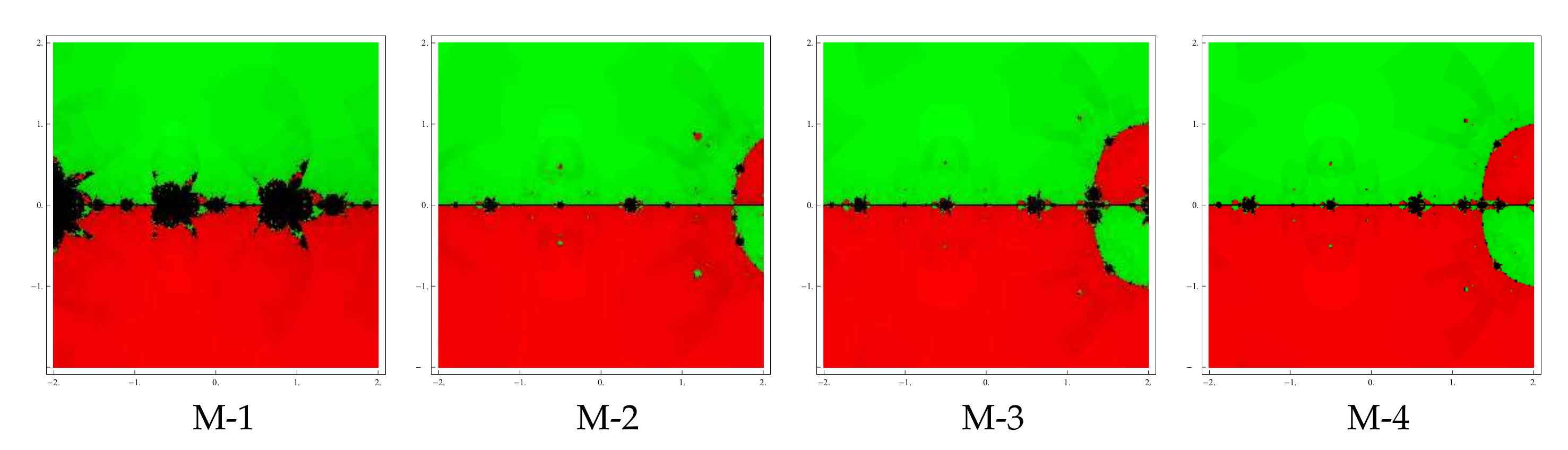
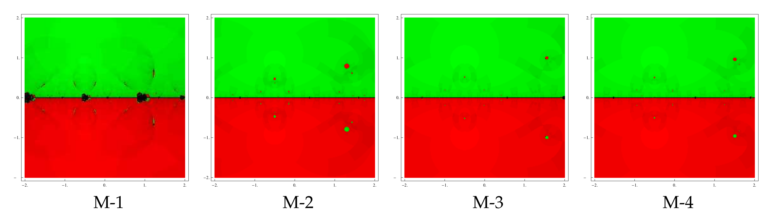
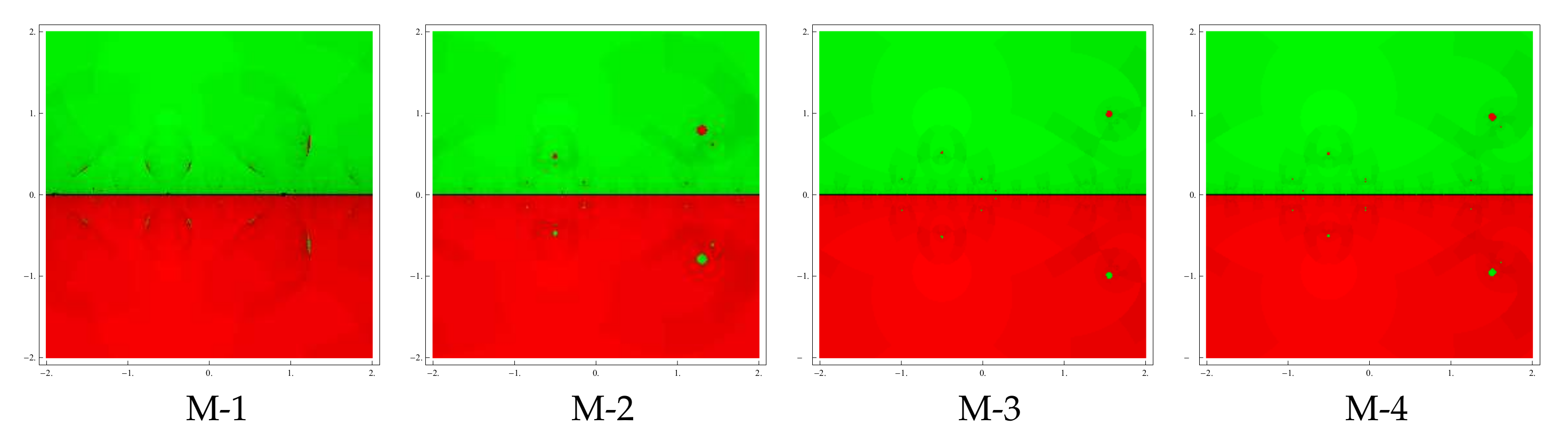
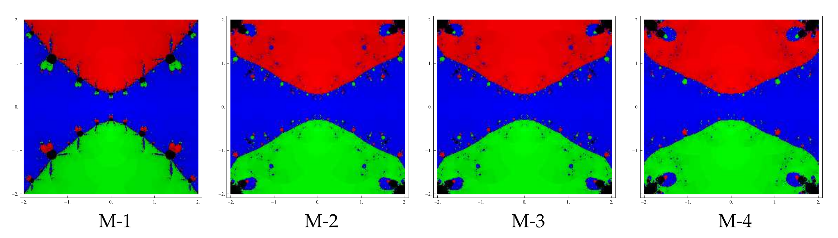
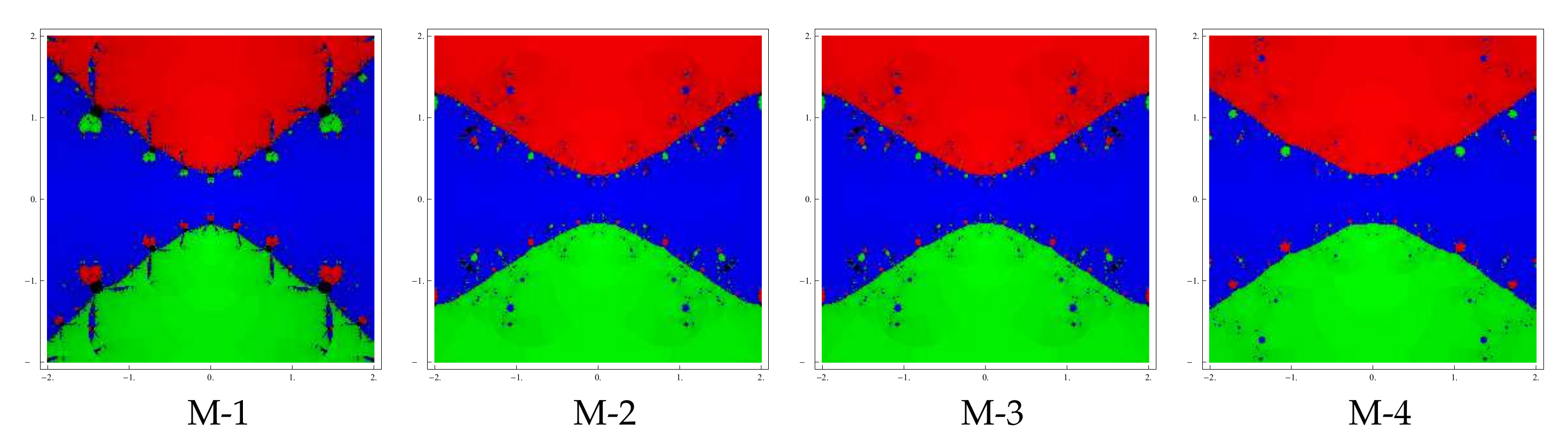
Test problem 1. Consider the polynomial ${\psi }_1\left(z\right)={(z^2+z+1)}^2$ having two zeros $\{-0.5-0.866025i,-0.5+0.866025i\}$ with multiplicity $\mu =2$. The attraction basins for this polynomial are shown in Figure 1, Figure 2 and Figure 3 corresponding to the choices $0.01,{10}^{-4},{10}^{-6}$ of parameter $\beta$. A color is assigned to each basin of attraction of a zero. In particular, red and green colors have been allocated to the basins of attraction of the zeros $-0.5-0.866025i$ and $-0.5+0.866025i$, respectively.

Figure 1. Basins of attraction by M-1–M-4 $(\beta =0.01)$ for polynomial ${\psi }_1\left(z\right)$.

Figure 2. Basins of attraction by M-1–M-4 $(\beta ={10}^{-4})$ for polynomial ${\psi }_1\left(z\right)$.

Figure 3. Basins of attraction by M-1–M-4 $(\beta ={10}^{-6})$ for polynomial ${\psi }_1\left(z\right)$.

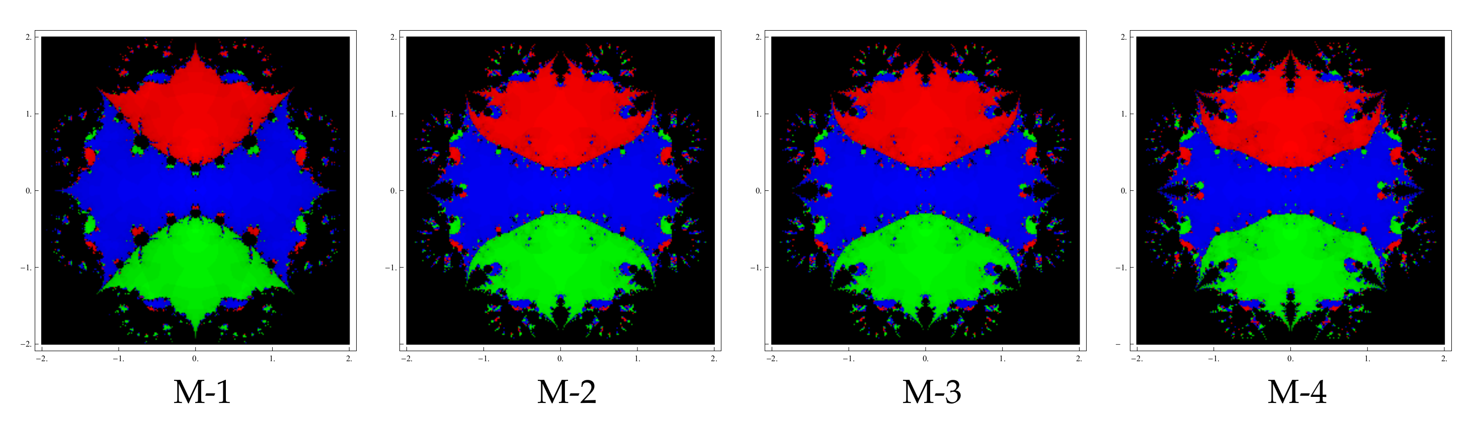
Test problem 2. Consider the polynomial ${\psi }_2\left(z\right)={\left(z^3+\frac{1}{4}z\right)}^3$ which has three zeros $\{-\frac{i}{2},\frac{i}{2},0\}$ with multiplicities $\mu =3$. Basins of attractors assessed by methods for this polynomial are drawn in Figure 4, Figure 5 and Figure 6 corresponding to choices $\beta =0.01,{10}^{-4},{10}^{-6}.$ The corresponding basin of a zero is identified by a color assigned to it. For example, green, red, and blue colors have been assigned corresponding to $-\frac{i}{2}$, $\frac{i}{2}$, and 0.

Figure 4. Basins of attraction by M-1–M-4 $(\beta =0.01)$ for polynomial ${\psi }_2\left(z\right)$.

Figure 5. Basins of attraction by M-1–M-4 $(\beta ={10}^{-4})$ for polynomial ${\psi }_2\left(z\right)$.

Figure 6. Basins of attraction by methods M-1–M-4 $(\beta ={10}^{-6})$ for polynomial ${\psi }_2\left(z\right)$.

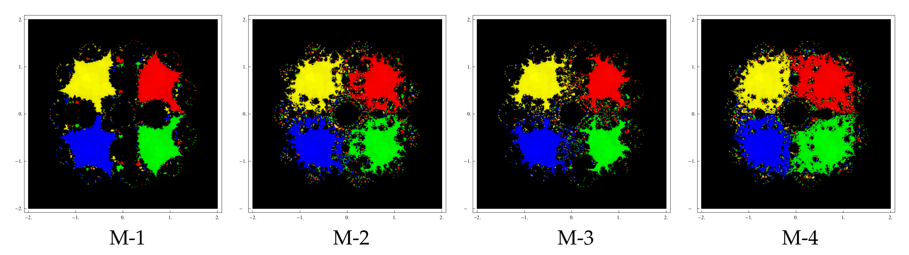
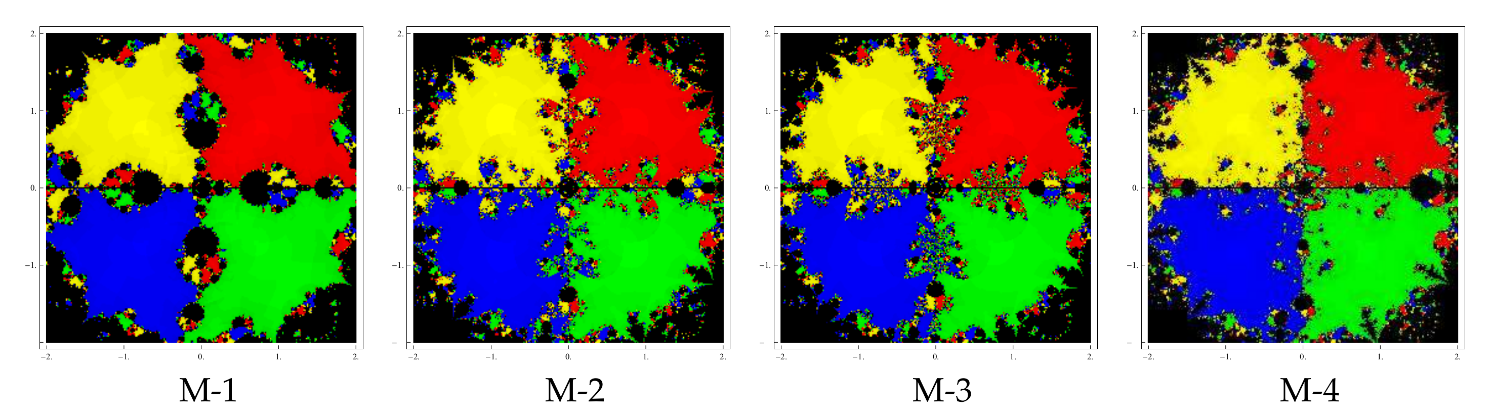
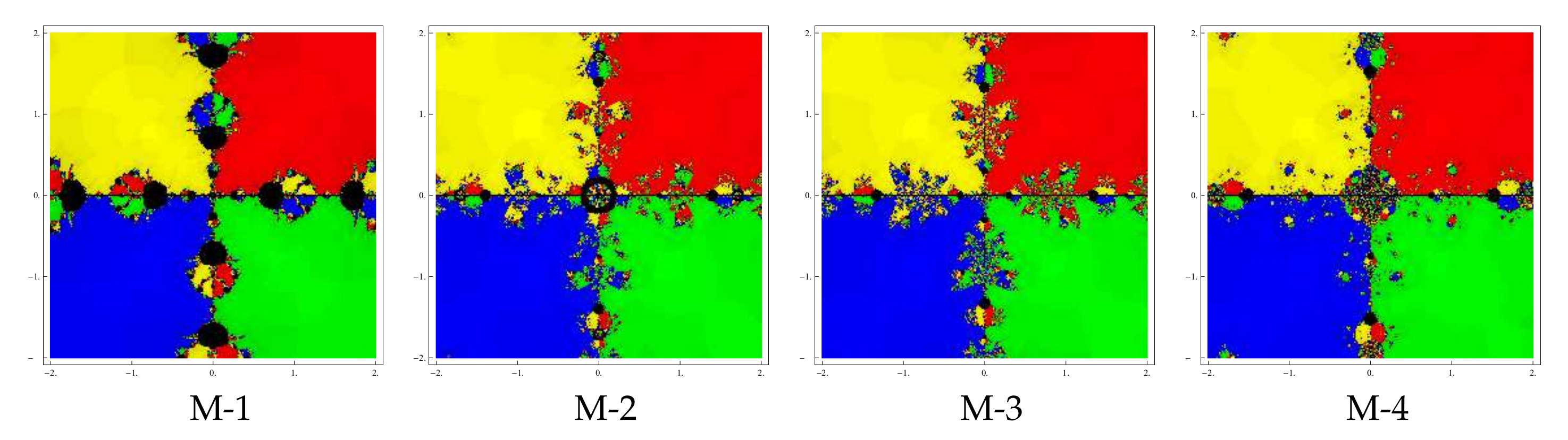
Test problem 3. Next, let us consider the polynomial ${\psi }_3\left(z\right)={\left(z^3+\frac{1}{z}\right)}^4$ that has four zeros $\{-0.707107+0.707107i,-0.707107-0.707107i,0.707107+0.707107i,0.707107-0.707107i\}$ with multiplicity $\mu =4$. The basins of attractors of zeros are shown in Figure 7, Figure 8 and Figure 9, for choices of the parameter $\beta =0.01,{10}^{-4},{10}^{-6}.$ A color is assigned to each basin of attraction of a zero. In particular, we assign yellow, blue, red, and green colors to $-0.707107+0.707107i$, $-0.707107-0.707107i$, $0.707107+0.707107i$ and $0.707107-0.707107i$, respectively.

Figure 7. Basins of attraction by M-1–M-4 $(\beta =0.01)$ for polynomial ${\psi }_3\left(z\right)$.

Figure 8. Basins of attraction by M-1–M-4 $(\beta ={10}^{-4})$ for polynomial ${\psi }_3\left(z\right)$.

Figure 9. Basins of attraction by M-1–M-4 $(\beta ={10}^{-6})$ for polynomial ${\psi }_3\left(z\right)$.

Estimation of $\beta$ values plays an important role in the selection of those members of family (3) which possess good convergence behavior. This is also the reason why different values of $\beta$ have been chosen to assess the basins. The above graphics clearly indicate that basins are becoming wider with the smaller values of parameter $\beta$. Moreover, the black zones (used to indicate divergence zones) are also diminishing as $\beta$ assumes small values. Thus, we conclude this section with a remark that the convergence of proposed methods is better for smaller values of parameter $\beta$.

5. Numerical Results

In order to validate of theoretical results that have been shown in previous sections, the new methods M1, M2, M3, and M4 are tested numerically by implementing them on some nonlinear equations. Moreover, these are compared with some existing optimal fourth order Newton-like methods. For example, we consider the methods by Li–Liao–Cheng [7], Li–Cheng–Neta [8], Sharma–Sharma [9], Zhou–Chen–Song [10], Soleymani–Babajee–Lotfi [12], and Kansal–Kanwar–Bhatia [14]. The methods are expressed as follows:

Li–Liao–Cheng method (LLCM):

$$\begin{array}{cc}\hfill z_k=& u_k-\frac{2\mu }{\mu +2}\frac{\psi \left(u_k\right)}{{\psi }^{\prime }\left(u_k\right)},\hfill \\ \hfill u_{k+1}=& u_k-\frac{\mu (\mu -2){\left(\frac{\mu }{\mu +2}\right)}^{-\mu }{\psi }^{\prime }\left(z_k\right)-{\mu }^2{\psi }^{\prime }\left(u_k\right)}{{\psi }^{\prime }\left(u_k\right)-{\left(\frac{\mu }{\mu +2}\right)}^{-\mu }{\psi }^{\prime }\left(z_k\right)}\frac{\psi \left(u_k\right)}{2{\psi }^{\prime }\left(u_k\right)}.\hfill \end{array}$$

Li–Cheng–Neta method (LCNM):

$$\begin{array}{cc}\hfill z_k=& u_k-\frac{2\mu }{\mu +2}\frac{\psi \left(u_k\right)}{{\psi }^{\prime }\left(u_k\right)},\hfill \\ \hfill u_{k+1}=& u_k-{\alpha }_1\frac{\psi \left(u_k\right)}{{\psi }^{\prime }\left(z_k\right)}-\frac{\psi \left(u_k\right)}{{\alpha }_2{\psi }^{\prime }\left(u_k\right)+{\alpha }_3{\psi }^{\prime }\left(z_k\right)},\hfill \end{array}$$

where

$$\begin{array}{cc}\hfill {\alpha }_1=& -\frac{1}{2}\frac{{\left(\frac{\mu }{\mu +2}\right)}^{\mu }\mu ({\mu }^4+4{\mu }^3-16\mu -16)}{{\mu }^3-4\mu +8},\hfill \\ \hfill {\alpha }_2=& -\frac{{({\mu }^3-4\mu +8)}^2}{\mu ({\mu }^4+4{\mu }^3-4{\mu }^2-16\mu +16)({\mu }^2+2\mu -4)},\hfill \\ \hfill {\alpha }_3=& \frac{{\mu }^2({\mu }^3-4\mu +8)}{{\left(\frac{\mu }{\mu +2}\right)}^{\mu }({\mu }^4+4{\mu }^3-4{\mu }^2-16\mu +16)({\mu }^2+2\mu -4)}.\hfill \end{array}$$

Sharma–Sharma method (SSM):

$$\begin{array}{cc}\hfill z_k=& u_k-\frac{2\mu }{\mu +2}\frac{\psi \left(u_k\right)}{{\psi }^{\prime }\left(u_k\right)},\hfill \\ \hfill u_{k+1}=& u_k-\frac{\mu }{8}[({\mu }^3-4\mu +8)-{(\mu +2)}^2{\left(\frac{\mu }{\mu +2}\right)}^{\mu }\frac{{\psi }^{\prime }\left(u_k\right)}{{\psi }^{\prime }\left(z_k\right)}\hfill \\ \hfill & \times \left(2(\mu -1)-(\mu +2){\left(\frac{\mu }{\mu +2}\right)}^{\mu }\frac{{\psi }^{\prime }\left(u_k\right)}{{\psi }^{\prime }\left(z_k\right)}\right)]\frac{\psi \left(u_k\right)}{{\psi }^{\prime }\left(u_k\right)}.\hfill \end{array}$$

Zhou–Chen–Song method (ZCSM):

$$\begin{array}{cc}\hfill z_k=& u_k-\frac{2\mu }{\mu +2}\frac{\psi \left(u_k\right)}{{\psi }^{\prime }\left(u_k\right)},\hfill \\ \hfill u_{k+1}=& u_k-\frac{\mu }{8}[{\mu }^3{\left(\frac{\mu +2}{\mu }\right)}^{2\mu }{\left(\frac{{\psi }^{\prime }\left(z_k\right)}{{\psi }^{\prime }\left(u_k\right)}\right)}^2-2{\mu }^2(\mu +3){\left(\frac{\mu +2}{\mu }\right)}^{\mu }\frac{{\psi }^{\prime }\left(z_k\right)}{{\psi }^{\prime }\left(u_k\right)}\hfill \\ \hfill & +({\mu }^3+6{\mu }^2+8\mu +8)]\frac{\psi \left(u_k\right)}{{\psi }^{\prime }\left(u_k\right)}.\hfill \end{array}$$

Soleymani–Babajee–Lotfi method (SBLM):

$$\begin{array}{cc}\hfill z_k=& u_k-\frac{2\mu }{\mu +2}\frac{\psi \left(u_k\right)}{{\psi }^{\prime }\left(u_k\right)},\hfill \\ \hfill u_{k+1}=& u_k-\frac{{\psi }^{\prime }\left(z_k\right)\psi \left(u_k\right)}{q_1{\left({\psi }^{\prime }\left(z_k\right)\right)}^2+q_2{\psi }^{\prime }\left(z_k\right){\psi }^{\prime }\left(u_k\right)+q_3{\left({\psi }^{\prime }\left(u_k\right)\right)}^2},\hfill \end{array}$$

where $q_1=\frac{1}{16}{\mu }^{3-\mu }{(\mu +2)}^{\mu },$$q_2=\frac{8-\mu (\mu +2)({\mu }^2-2)}{8\mu },$$q_3=\frac{1}{16}(\mu -2){\mu }^{\mu -1}{(\mu +2)}^{3-\mu }$.

Kansal–Kanwar–Bhatia method (KKBM):

$$\begin{array}{cc}\hfill z_k=& u_k-\frac{2\mu }{\mu +2}\frac{\psi \left(u_k\right)}{{\psi }^{\prime }\left(u_k\right)},\hfill \\ \hfill u_{k+1}=& u_k-\frac{\mu }{4}\psi \left(u_k\right)\left(1+\frac{{\mu }^4{p}^{-2\mu }{\left(p^{\mu -1}-\frac{{\psi }^{\prime }\left(z_k\right)}{{\psi }^{\prime }\left(u_k\right)}\right)}^2(p^{\mu }-1)}{8(2p^{\mu }+n(p^{\mu }-1))}\right)\hfill \\ \hfill & \times \left(\frac{4-2\mu +{\mu }^2(p^{-\mu }-1)}{{\psi }^{\prime }\left(u_k\right)}-\frac{p^{-\mu }{(2p^{\mu }+\mu (p^{\mu }-1))}^2}{{\psi }^{\prime }\left(u_k\right)-{\psi }^{\prime }\left(z_k\right)}\right),\hfill \end{array}$$

where $p=\frac{\mu }{\mu +2}.$

Computations are performed in the programming package of Mathematica software [20] in a PC with specifications: Intel(R) Pentium(R) CPU B960 @ 2.20 GHz, 2.20 GHz (32-bit Operating System) Microsoft Windows 7 Professional and 4 GB RAM. Numerical tests are performed by choosing the value $-0.01$ for parameter $\beta$ in new methods. The tabulated results of the methods displayed in Table 1 include: (i) iteration number $\left(k\right)$ required to obtain the desired solution satisfying the condition $|u_{k+1}-u_k|+|\psi \left(u_k\right)|<{10}^{-100}$, (ii) estimated error $|u_{k+1}-u_k|$ in the consecutive first three iterations, (iii) calculated convergence order (CCO), and (iv) time consumed (CPU time in seconds) in execution of a program, which is measured by the command “TimeUsed[ ]”. The calculated convergence order (CCO) is computed by the well-known formula (see [24])

$$\mathrm{CCO}=\frac{log|(u_{k+2}-\alpha )/(u_{k+1}-\alpha )|}{log|(u_{k+1}-\alpha )/(u_k-\alpha )|},\mathrm{for}\mathrm{each}k=1,2,\dots$$

(37)

Table 1. Comparison of numerical results.

Methods	k	$|{\mathit{u}}_2-{\mathit{u}}_1|$	$|{\mathit{u}}_3-{\mathit{u}}_2|$	$|{\mathit{u}}_4-{\mathit{u}}_3|$	CCO	CPU-Time
${\psi }_1\left(u\right)$
LLCM	6	$7.84\times {10}^{-2}$	$6.31\times {10}^{-3}$	$1.06\times {10}^{-5}$	4.000	0.0784
LCNM	6	$7.84\times {10}^{-2}$	$6.31\times {10}^{-3}$	$1.006\times {10}^{-5}$	4.000	0.0822
SSM	6	$7.99\times {10}^{-2}$	$6.78\times {10}^{-3}$	$1.44\times {10}^{-5}$	4.000	0.0943
ZCSM	6	$8.31\times {10}^{-2}$	$7.83\times {10}^{-3}$	$2.76\times {10}^{-5}$	4.000	0.0956
SBLM	6	$7.84\times {10}^{-2}$	$6.31\times {10}^{-3}$	$1.06\times {10}^{-5}$	4.000	0.0874
KKBM	6	$7.74\times {10}^{-2}$	$5.97\times {10}^{-3}$	$7.31\times {10}^{-6}$	4.000	0.0945
M1	6	$9.20\times {10}^{-2}$	$1.16\times {10}^{-2}$	$1.16\times {10}^{-4}$	4.000	0.0774
M2	6	$6.90\times {10}^{-2}$	$3.84\times {10}^{-3}$	$1.03\times {10}^{-6}$	4.000	0.0794
M3	6	$6.21\times {10}^{-2}$	$2.39\times {10}^{-3}$	$7.06\times {10}^{-8}$	4.000	0.0626
M4	6	$6.29\times {10}^{-2}$	$2.54\times {10}^{-3}$	$9.28\times {10}^{-8}$	4.000	0.0785
${\psi }_2\left(u\right)$
LLCM	4	$2.02\times {10}^{-4}$	$2.11\times {10}^{-17}$	$2.51\times {10}^{-69}$	4.000	0.7334
LCNM	4	$2.02\times {10}^{-4}$	$2.12\times {10}^{-17}$	$2.54\times {10}^{-69}$	4.000	1.0774
SSM	4	$2.02\times {10}^{-4}$	$2.12\times {10}^{-17}$	$2.60\times {10}^{-69}$	4.000	1.0765
ZCSM	4	$2.02\times {10}^{-4}$	$2.15\times {10}^{-17}$	$2.75\times {10}^{-69}$	4.000	1.1082
SBLM	4	$2.02\times {10}^{-4}$	$2.13\times {10}^{-17}$	$2.62\times {10}^{-69}$	4.000	1.2950
KKBM	4	$2.02\times {10}^{-4}$	$2.08\times {10}^{-17}$	$2.31\times {10}^{-69}$	4.000	1.1548
M1	4	$1.01\times {10}^{-4}$	$1.08\times {10}^{-18}$	$1.43\times {10}^{-74}$	4.000	0.5612
M2	4	$9.85\times {10}^{-5}$	$4.94\times {10}^{-19}$	$3.13\times {10}^{-76}$	4.000	0.5154
M3	4	$9.85\times {10}^{-5}$	$4.94\times {10}^{-19}$	$3.13\times {10}^{-76}$	4.000	0.5311
M4	4	$9.82\times {10}^{-5}$	$4.35\times {10}^{-19}$	$1.67\times {10}^{-76}$	4.000	0.5003
${\psi }_3\left(u\right)$
LLCM	4	$4.91\times {10}^{-5}$	$5.70\times {10}^{-21}$	$1.03\times {10}^{-84}$	4.000	0.6704
LCNM	4	$4.91\times {10}^{-5}$	$5.70\times {10}^{-21}$	$1.03\times {10}^{-84}$	4.000	0.9832
SSM	4	$4.92\times {10}^{-5}$	$5.71\times {10}^{-21}$	$1.04\times {10}^{-84}$	4.000	1.0303
ZCSM	4	$4.92\times {10}^{-5}$	$5.72\times {10}^{-21}$	$1.05\times {10}^{-84}$	4.000	1.0617
SBLM	4	$4.92\times {10}^{-5}$	$5.73\times {10}^{-21}$	$1.06\times {10}^{-84}$	4.000	1.2644
KKBM	4	$4.91\times {10}^{-5}$	$5.66\times {10}^{-21}$	$1.00\times {10}^{-84}$	4.000	1.0768
M1	3	$6.35\times {10}^{-6}$	$2.73\times {10}^{-25}$	0	4.000	0.3433
M2	3	$4.94\times {10}^{-6}$	$6.81\times {10}^{-26}$	0	4.000	0.2965
M3	3	$5.02\times {10}^{-6}$	$7.46\times {10}^{-26}$	0	4.000	0.3598
M4	3	$4.77\times {10}^{-6}$	$5.66\times {10}^{-26}$	0	4.000	0.3446
${\psi }_4\left(u\right)$
LLCM	4	$1.15\times {10}^{-4}$	$5.69\times {10}^{-17}$	$3.39\times {10}^{-66}$	4.000	1.4824
LCNM	4	$1.15\times {10}^{-4}$	$5.70\times {10}^{-17}$	$3.40\times {10}^{-66}$	4.000	2.5745
SSM	4	$1.15\times {10}^{-4}$	$5.71\times {10}^{-17}$	$3.44\times {10}^{-66}$	4.000	2.5126
ZCSM	4	$1.15\times {10}^{-4}$	$5.72\times {10}^{-17}$	$3.47\times {10}^{-66}$	4.000	2.5587
SBLM	4	$1.15\times {10}^{-4}$	$5.83\times {10}^{-17}$	$3.79\times {10}^{-66}$	4.000	3.1824
KKBM	4	$1.15\times {10}^{-4}$	$5.63\times {10}^{-17}$	$3.21\times {10}^{-66}$	4.000	2.4965
M1	4	$4.18\times {10}^{-4}$	$6.03\times {10}^{-19}$	$2.60\times {10}^{-74}$	4.000	0.4993
M2	4	$3.88\times {10}^{-5}$	$2.24\times {10}^{-19}$	$2.45\times {10}^{-76}$	4.000	0.5151
M3	4	$3.92\times {10}^{-5}$	$2.57\times {10}^{-19}$	$4.80\times {10}^{-76}$	4.000	0.4996
M4	4	$3.85\times {10}^{-5}$	$1.92\times {10}^{-19}$	$1.18\times {10}^{-76}$	4.000	0.4686
${\psi }_5\left(u\right)$
LLCM	4	$2.16\times {10}^{-4}$	$3.17\times {10}^{-17}$	$1.48\times {10}^{-68}$	4.000	1.9042
LCNM	4	$2.16\times {10}^{-4}$	$3.17\times {10}^{-17}$	$1.47\times {10}^{-68}$	4.000	2.0594
SSM	4	$2.16\times {10}^{-4}$	$3.16\times {10}^{-17}$	$1.45\times {10}^{-68}$	4.000	2.0125
ZCSM	4	$2.16\times {10}^{-4}$	$3.15\times {10}^{-17}$	$1.43\times {10}^{-68}$	4.000	2.1530
SBLM	4	$2.16\times {10}^{-4}$	$3.01\times {10}^{-17}$	$1.15\times {10}^{-68}$	4.000	2.4185
KKBM	4	$2.16\times {10}^{-4}$	$3.24\times {10}^{-17}$	$1.63\times {10}^{-68}$	4.000	2.2153
M1	4	$2.48\times {10}^{-4}$	$7.62\times {10}^{-21}$	$6.81\times {10}^{-83}$	4.000	1.6697
M2	4	$2.15\times {10}^{-5}$	$2.03\times {10}^{-21}$	$1.63\times {10}^{-85}$	4.000	1.7793
M3	4	$2.19\times {10}^{-5}$	$2.51\times {10}^{-21}$	$4.35\times {10}^{-85}$	4.000	1.7942
M4	4	$2.11\times {10}^{-5}$	$1.66\times {10}^{-21}$	$6.29\times {10}^{-86}$	4.000	1.6855

The problems considered for numerical testing are shown in Table 2.

Table 2. Test functions.

Functions		Root ($\mathit{\alpha }$)		Multiplicity		Initial Guess
${\psi }_1\left(u\right)=u^3-5.22u^2+9.0825u-5.2675$		1.75		2		2.4
${\psi }_2\left(u\right)=-\frac{u^4}{12}+\frac{u^2}{2}+u+e^u(u-3)+sinu+3$		0		3		0.6
${\psi }_3\left(u\right)={\left(e^{-u}-1+\frac{u}{5}\right)}^4$		4.9651142317…		4		5.5
${\psi }_4\left(u\right)=u(u^2+1)(2e^{u^2+1}+u^2-1){cosh}^4\left(\frac{\pi u}{2}\right)$		i		6		1.2 i
${\psi }_5\left(u\right)=[{tan}^{-1}\left(\frac{\sqrt{5}}{2}\right)-{tan}^{-1}\left(\sqrt{u^2-1}\right)+\sqrt{6}({tan}^{-1}\left(\sqrt{\frac{u^2-1}{6}}\right)$
$-{tan}^{-1}\left(\frac{1}{2}\sqrt{\frac{5}{6}}\right))-\frac{11}{63}{]}^7$		1.8411294068…		7		1.6

From the computed results in Table 1, we can observe the good convergence behavior of the proposed methods. The reason for good convergence is the increase in accuracy of the successive approximations as is evident from values of the differences $|u_{k+1}-u_k|$. This also implies to stable nature of the methods. Moreover, the approximations to solutions computed by the proposed methods have either greater or equal accuracy than those computed by existing counterparts. The value 0 of $|u_{k+1}-u_k|$ indicates that the stopping criterion $|u_{k+1}-u_k|+|\psi \left(u_k\right)|<{10}^{-100}$ has been satisfied at this stage. From the calculation of calculated convergence order as shown in the second last column in each table, we have verified the theoretical fourth order of convergence. The robustness of new algorithms can also be judged by the fact that the used CPU time is less than that of the CPU time by the existing techniques. This conclusion is also confirmed by similar numerical experiments on many other different problems.

6. Conclusions

We have proposed a family of fourth order derivative-free numerical methods for obtaining multiple roots of nonlinear equations. Analysis of the convergence has been carried out under standard assumptions, which proves the convergence order four. The important feature of our designed scheme is its optimal order of convergence which is rare to achieve in derivative-free methods. Some special cases of the family have been explored. These cases are employed to solve some nonlinear equations. The performance is compared with existing techniques of a similar nature. Testing of the numerical results have shown the presented derivative-free method as good competitors to the already established optimal fourth order techniques that use derivative information in the algorithm. We conclude this work with a remark: the proposed derivative-free methods can be a better alternative to existing Newton-type methods when derivatives are costly to evaluate.