Optimizing the Estimation of a Histogram-Bin Width—Application to the Multivariate Mixture-Model Estimation

Abstract

A maximum-likelihood estimation of a multivariate mixture model’s parameters is a difficult problem. One approach is to combine the REBMIX and EM algorithms. However, the REBMIX algorithm requires the use of histogram estimation, which is the most rudimentary approach to an empirical density estimation and has many drawbacks. Nevertheless, because of its simplicity, it is still one of the most commonly used techniques. The main problem is to estimate the optimum histogram-bin width, which is usually set by the number of non-overlapping, regularly spaced bins. For univariate problems it is usually denoted by an integer value; i.e., the number of bins. However, for multivariate problems, in order to obtain a histogram estimation, a regular grid must be formed. Thus, to obtain the optimum histogram estimation, an integer-optimization problem must be solved. The aim is therefore the estimation of optimum histogram binning, alone and in application to the mixture model parameter estimation with the REBMIX&EM strategy. As an estimator, the Knuth rule was used. For the optimization algorithm, a derivative based on the coordinate-descent optimization was composed. These proposals yielded promising results. The optimization algorithm was efficient and the results were accurate. When applied to the multivariate, Gaussian-mixture-model parameter estimation, the results were competitive. All the improvements were implemented in the rebmix R package.

1. Introduction

Let the random variable $\mathit{y}\in {\mathbb{R}}^d$ follow the multivariate, finite-mixture model with the probability density function

$$f\left(\mathit{y}\right|c,\mathit{w},\mathit{\Theta })=\sum _{l=1}^c{w}_l{f}_l\left(\mathit{y}\right|{\mathit{\Theta }}_l).$$

(1)

The main task is to estimate the $c,\mathit{w},\mathit{\Theta }$ parameters. The parameters $c,\mathit{w},\mathit{\Theta }$ are, respectively, the number of components in the mixture model, the component weights and the component parameters. The maximum-likelihood estimation of such parameters is a difficult task and mostly requires a combination of multiple procedures for its estimation [1]. Obtaining a direct analytical derivation of the likelihood function for mixture models is difficult and inconvenient; thus, instead, the complete-data-likelihood function can be used and the maximum-likelihood parameter estimates can be obtained using the expectation-maximization (EM) algorithm [2]. However, to use the EM algorithm and obtain reasonable maximum-likelihood estimates we should provide a good initialization of the EM algorithm [3,4]. Furthermore, as the number of components c can be seen as a complexity parameter, the value of the likelihood function increases as this value increases, making the selection in the maximum-likelihood framework problematic. Thus, the selection of the simplest model from the many available via a model-selection procedure is necessary [1]. This and the already-mentioned initialization of the EM algorithm additionally harden the problem. Such a feeling can be obtained by inspecting the sizable body of literature on estimating mixture-model parameters [3,4,5,6]. The research goes from multiple random initialization of the EM algorithm [3] to stand-alone heuristics, such as the procedures described in [5,6].

The use of the rough-enhanced-Bayes mixture-estimation (REBMIX) algorithm for estimating the mixture-model parameters can be fruitful [7,8,9]. Either as a stand-alone procedure [10] or in conjunction with the EM algorithm [4], the benefits are clear. In the former case it is fast and robust, whereas in the latter, when used with EM, it gives a good initialization and accelerates the estimation process by reducing the number of EM iterations needed for convergence. Since the REBMIX is a data-based heuristic, it encompasses some simple non-parametric density-estimation methods, such as the histogram estimation, as a preprocessing step. The histogram estimation or other preprocessing techniques used in [9] requires some smoothing parameters for the input, referred to as the number of bins v. This parameter is, as was discussed in [4], usually not known; however, as it is an integer-valued parameter, some plausible range can be used and many mixture-model parameters can be estimated, from which the best can be chosen via model selection. Although it is always good to check multiple possible solutions, this can bring a lot of unwanted overhead in terms of the computational time. In some specific cases the amount of time available, or, simply, the amount we want to invest, is limited, whereas the need for high accuracy is always a requirement [11].

Three strategies were derived in a study of the utilization of the REBMIX algorithm as an improved initialization technique for the EM algorithm in [4]: the exhaustive REBMIX&EM, best REBMIX&EM and single REBMIX&EM strategies. The exhaustive REBMIX&EM, as the name suggests, exhaustively utilizes the EM algorithm for every solution obtained by the REBMIX algorithm. This strategy is useful since the smoothing parameter for the REBMIX preprocessing is not known in advance and the ordered range of integer numbers K makes possible estimations of the different mixture-model parameters. On the other hand, the computational demands of this strategy are fairly high, and therefore, the best REBMIX&EM strategy is presented, which has a much smaller computational footprint. A reduction has been made in the sense that instead of using the EM algorithm for every solution obtained from the REBMIX algorithm, the EM is utilized on a smaller number of best candidates obtained from REBMIX. They are then used for the model selection, from which the optimum is selected. However, in both of these strategies the smoothing parameter for the REBMIX algorithm is unknown and the overhead for running the REBMIX algorithm on all the smoothing-parameter values from the ordered set of numbers K is present. This can, after all, be reduced if the optimum number of bins v is somehow known in advance and used as the input for the single REBMIX&EM strategy.

Additionally, to keep the amount of time reasonable, for the multivariate, mixture-model parameter estimation, the smoothing parameter, e.g., the number of bins v for the histogram estimation, is kept constant for each dimension of the problem. This can be very limiting. Nonetheless, the increase in the computational requirement can hardly be justified if all the possible combinations for multivariate datasets are considered. The histogram grid in the multivariate settings can be seen as a tessellation of a flat surface. In other words, a regular grid must be formed, where the tiles are most often hyper-rectangles with sides $\mathit{h}=\{h_1,h_2,\dots ,h_d\}$. The estimation of the histogram-bin width requires an estimation of all the histogram-bin widths ${\mathit{h}}_{ij}$ for every bin j in the multidimensional histogram grid.

In this paper we tackle the problem of estimating the optimum histogram-bin width for a multivariate setting applied to the mixture-model parameter estimation with the REBMIX&EM strategy. Instead of focusing on the estimator of the optimum histogram-bin width, our main focus is on an efficient estimation of the optimum histogram-bin-width using a known estimator. We introduce our problem as an integer-optimization problem and derive the optimization procedure for its solution. In order to present the benefits we apply the proposal, first solely as a histogram-bin width estimation, and secondly, for a multivariate, Gaussian mixture-model parameter estimation with the REBMIX&EM strategy. The results obtained showed the benefits of our proposal in terms of efficacy and accuracy.

The rest of the paper is structured as follows. Section 2 is reserved for some theoretical insights into the Gaussian mixture-model parameter estimation. We chose the Gaussian mixture models because they are the most commonly used type of mixture model. We present the state-of-the-art model-selection procedure for the Gaussian mixture-model parameter estimation in a maximum-likelihood framework, and discuss the computational complexity and compare it to the REBMIX&EM computational requirements. Additionally, we give some theoretical benefits in terms of the computational efficacy of using the single REBMIX&EM strategy instead of the best REBMIX&EM strategy. Section 3 gives a description of the histogram estimation, the main problem statement and our proposal for its solution. Section 4 is reserved for an explanation of the numerical experiments used to obtain some empirical insights into the accuracy and efficacy of our proposal. Section 5 demonstrates the main results and Section 6 presents some discussion of the main empirical results. Finally, we end this paper with concluding remarks in Section 7.

2. Gaussian Mixture-Model Parameter Estimation

Let the random variable $\mathit{y}\in {\mathbb{R}}^d$ follow the multivariate, Gaussian mixture model with the probability density function

$$f\left(\mathit{y}\right|c,\mathit{w},\mathit{\Theta })=\sum _{l=1}^c{w}_l{f}_l\left(\mathit{y}\right|{\mathit{\Theta }}_l),$$

(2)

where

$$f_l\left(\mathit{y}\right|{\mathit{\Theta }}_l)=\frac{1}{\sqrt{{\left(2\pi \right)}^d\left|{\Sigma }_l\right|}}exp\left(-\frac{1}{2}(\mathit{y}-{\mu }_l){\Sigma }_l^{-1}{(\mathit{y}-{\mu }_l)}^T\right)$$

(3)

is the multivariate Gaussian probability density function. In other words, the Gaussian mixture-model probability density function is a linear combination of multiple Gaussian probability density functions with different parameters (mean vector ${\mu }_l$ and covariance matrix ${\Sigma }_l$ ), usually referred to as components [1]. The parameter c is the number of components and $\mathit{w}$ are the component weights. The weights of the components $\mathit{w}=\{w_1,w_2,\dots ,w_c\}$ have the properties of the convex combination $w_l\ge 0\wedge {\sum }_{l=1}^c{w}_l=1$. The component parameters can be summarized as $\mathit{\Theta }=\{{\mathit{\Theta }}_1,\dots ,{\mathit{\Theta }}_c\}=\{\{{\mu }_1,{\Sigma }_1\},\dots ,\{{\mu }_c,{\Sigma }_c\}\}$. The maximum-likelihood estimation of the parameters $c,\mathit{w},\mathit{\Theta }$ can be summarized as

$$c_{\mathrm{opt}},{\mathit{w}}_{\mathrm{opt}},{\mathit{\Theta }}_{\mathrm{opt}}=\underset{c,\mathit{w},\mathit{\Theta }}{\mathrm{argmax}}L(c,\mathit{w},\mathit{\Theta }|\mathit{Y}),$$

(4)

where

$$L(c,\mathit{w},\mathit{\Theta }|\mathit{Y})=\prod _{j=1}^{n}f\left({\mathit{y}}_j\right|c,\mathit{w},\mathit{\Theta })$$

(5)

is the likelihood function and $\mathit{Y}=\{{\mathit{y}}_1,{\mathit{y}}_2,\dots ,{\mathit{y}}_n\}$ is the dataset containing n observations for which the parameters are being estimated.

Remark 1.

The likelihood function L defined in Equation (5) assumes that the observations from the dataset $\mathit{Y}$ are independent and identically distributed (i.i.d). Additionally, instead of using the likelihood function L defined in Equation (5), often, the log-likelihood function $logL(c,\mathit{w},\mathit{\Theta }|\mathit{Y})={\sum }_{j=1}^{n}logf\left({\mathit{y}}_j\right|c,\mathit{w},\mathit{\Theta })$ is used for a maximum-likelihood estimation of the parameters since the log is a monotonically increasing function.

2.1. Brief Information about the Notation in the Following Paragraphs

There are a lot of parameters in the Gaussian mixture model. The actual number of parameters can be calculated and is $M=c-1+cd+cd(d+1)/2$, where c is the number of components and d is the number of dimensions in the multivariate case. For convenience and simplicity we will use the following notation: the parameters $\mathit{w}$ and $\mathit{\Theta }$ can be written as $\mathit{w}\left(c\right)$ and $\mathit{\Theta }\left(c\right)$, as they are both dependent on the number of components c. However, the optimum estimated (selected) parameters, ${\mathit{w}}_{\mathrm{opt}}$ and ${\mathit{\Theta }}_{\mathrm{opt}}$, will not be written in the above-described manner, as it will be clear to which number of components $c_{\mathrm{opt}}$ they refer.

2.2. EM Algorithm

Maximum-likelihood estimates can be obtained with the EM algorithm [2]. EM utilizes two steps, i.e., the expectation (E) and maximization (M) steps iteratively until the convergence is achieved, as described in Algorithm 1. In the E step the posterior probability ${\tau }_{lj}$ that the observation ${\mathit{y}}_j$ from $\mathit{Y}$ arose from the lth component is calculated. This results in a $n\times c$ matrix $\mathit{T}$ for the dataset $\mathit{Y}$ with n observations and a Gaussian mixture model with c components. In the M step the iteration-wise update equations for the parameters can be derived by maximizing the conditional expectation of the complete-data log-likelihood function [1]. The update equations for the E and M steps of the EM algorithm can be found in a lot of literaturel for example, in [1] or [4]. Hence, they will be omitted here.

Algorithm 1: EM algorithm.

1:  Input dataset $\mathit{Y}$, initialize $c,\mathit{w}\left(c\right)$, $\mathit{\Theta }\left(c\right)$, set the threshold $ϵ$, maximum number of iterations $I_{max}$; 2:  Set $c_{\mathrm{opt}}=c$, ${\mathit{w}}_{\mathrm{opt}}=\mathit{w}\left(c\right)$, ${\mathit{\Theta }}_{\mathrm{opt}}=\mathit{\Theta }\left(c\right)$, $I=0$; 3:  do: 4:    $\mathit{w}\left(c\right)={\mathit{w}}_{\mathrm{opt}}$, $\mathit{\Theta }\left(c\right)={\mathit{\Theta }}_{\mathrm{opt}}$; 5:    $\mathit{T}=\mathrm{EStep}(\mathit{Y},\mathit{w}(c),\mathit{\Theta }(c\left)\right)$; 6:    ${\mathit{w}}_{\mathrm{opt}},{\mathit{\Theta }}_{\mathrm{opt}}$ = MStep($\mathit{Y},\mathit{T},\mathit{w}\left(c\right),\mathit{\Theta }\left(c\right)$); 7:    $I=I+1$; 8:  while $|logL(c_{\mathrm{opt}},{\mathit{w}}_{\mathrm{opt}},{\mathit{\Theta }}_{\mathrm{opt}}|\mathit{Y})-logL(c,\mathit{w}\left(c\right),\mathit{\Theta }\left(c\right)|\mathit{Y})|>ϵ\vee I\le I_{max}$;

Remark 2.

Admitting the absolute change in the log-likelihood function is the most used and straightforward criterion for the EM’s convergence; the relative change in log-likelihood function or the change in the parameter values can be used to assess the convergence and stop the EM algorithm. Additionally, as the log-likelihood function for the Gaussian mixture model is unbounded, i.e., $|{\Sigma }_l|\to 0\Rightarrow logL(c,\mathit{w},\mathit{\Theta }|\mathit{Y})\to \infty$, the EM algorithm, when supplied with bad initial parameters, can converge, painfully, slowly, to this degenerated (singular) solution. Although there are quite a few remedies for this problem, such as using a regularization [3,12] or parsimonious covariance structure [13,14], which can bound the log-likelihood function by bounding the parameter space, here, as the main remedy, the maximum allowed number of iterations $I_{max}$ of the EM algorithm is used. If the maximum allowed number of iterations is exhausted, the obtained solution will be considered as the optimum.

2.3. Model-Selection Procedure

The EM is a hill-climbing algorithm. Starting from some initially supplied parameters, in each iteration the algorithm increases the value of the likelihood function (Equation (5)) until some sort of convergence is achieved. However, in the case of a non-convex optimization function, such as the log-likelihood function for a Gaussian mixture model and generally all mixture models, the final estimated parameters can be non-promising or even degenerated (see Remark 2) based on the initial starting parameters and the spurious local optima that are maximized. As the likelihood function for the mixture models, especially Gaussian mixture models, contains many modes, hitting global optima is most likely computationally not unjustified, even if some techniques other than the EM algorithm are used [1,15]. Therefore, the search space is narrowed by introducing the model-selection procedure, described in Algorithm 2. This can be done as the number of components with the following properties $c\in \mathbb{Z}\wedge c\ge 1$ represents the complexity parameter of the Gaussian mixture model (and all other mixture models) and selecting the simplest model with respect to the parameter c should always be preferred [1]. Thus, the problem is separated into multiple simpler problems, and amongst all of the solutions, the best is chosen via the estimator, which is called the information criterion [1]. The information-criteria estimators that are mostly used in the context of a Gaussian mixture-model selection procedure rely on an estimated maximum value of the likelihood function [1,4].

Remark 3.

In some extremely rare cases, the number of components c of the mixture model is known in advance, and the model-selection procedure above-described and illustrated in Algorithm 2 is obsolete.

Algorithm 2: Model selection procedure.

1:  Input dataset $\mathit{Y}$, initialize set $C=\{c_1,c_2,\dots \}$; 2:  ${\mathrm{IC}}_{\mathrm{opt}}=\infty$, ${\mathit{w}}_{\mathrm{opt}}=\left\{\right\}$, ${\mathit{\Theta }}_{\mathrm{opt}}=\left\{\right\}$, $c_{\mathrm{opt}}=0$; 3:  foreach $c\in C$ do: 4:    Initialize ${\mathit{w}}_{\mathrm{ini}}\left(c\right)$, ${\mathit{\Theta }}_{\mathrm{ini}}\left(c\right)$; 5:    $\mathit{w}\left(c\right),\mathit{\Theta }\left(c\right)$ = EM($\mathit{Y},{\mathit{w}}_{\mathrm{ini}}\left(c\right),{\mathit{\Theta }}_{\mathrm{ini}}\left(c\right)$); 6:    Estimate criterion $\mathrm{IC}=\mathrm{ICF}(\mathit{Y},\mathit{w}(c),\mathit{\Theta }(c\left)\right)$; 7:    if $\mathrm{IC}<{\mathrm{IC}}_{\mathrm{opt}}$: 8:       ${\mathrm{IC}}_{\mathrm{opt}}=\mathrm{IC}$, $c_{\mathrm{opt}}=c$, ${\mathit{w}}_{\mathrm{opt}}=\mathit{w}\left(c\right)$, ${\mathit{\Theta }}_{\mathrm{opt}}=\mathit{\Theta }\left(c\right)$; 9:    end 10:  end

Remark 4.

The literature contains a plethora of different information criteria used to assess the goodness of the estimated Gaussian mixture-model parameters (or any other mixture model) [1,4,9]. Hence, we used the general notation in line 6 of Algorithm 2. ICFstands for the estimator and IC is the estimated value. Although many of the information-criterion estimators assume the lower estimated value is better, there are estimators for which the higher estimated value is better (for example, the Approximate weight of evidence (AWE) used in [14] or the Bayesian information criterion (BIC) approximation used in [16]). These can also be used in Algorithm 2 by simply negating the estimated value (IC).

However, choosing several different values for the number of components c, as represented by set C in line 1 of Algorithm 2, can be troublesome. It is always better to use an ordered set of numbers of components ranging from some $c_{min}$ to $c_{max}$ so the change in the information-criterion estimator value can be smoother in respect to the change in the number of components c. Usually, for the sake of pure simplicity and to get rid of one additional user-defined parameter, the parameter $c_{min}$ can safely be assumed to be 1 [4]. That leads us to the model-selection procedure described in Algorithm 3. Additionally, some authors emphasize the multiple different initializations of the EM algorithm for a given number of components c, to ensure that the estimated parameters of the Gaussian mixture model yield the best possible local optima of the likelihood function [3,4]. Hence, the model-selection procedure described in Algorithm 3 reflects the state-of-the-art procedure for estimating the Gaussian mixture-model parameters (and also any other mixture-model parameters) [3,4,6,9,17,18].

To estimate the theoretical computational complexity of the above-mentioned procedure (Algorithm 3), it must be investigated with respect to three parameters: the number of observations in the dataset n, the number of dimensions d and the number of components c. From Algorithm 3 we can see that the main body of the model-selection procedure (lines 6, 7 and 8 of Algorithm 3) executes $r{c}_{max}$ times. The computational complexity of the EM algorithm, given in Algorithm 1, cannot be exactly estimated, as the EM does not have clear stopping criteria. However, by using our implementation, the upper bound is defined by the maximum number of iterations $I_{max}$. Therefore, the upper bound can be estimated as $O\left(I_{max}nc{d}^2\right)$, where $O\left(nc{d}^2\right)$ is the computational complexity of a single iteration of the EM algorithm, judging by the E and M step equations [4]. The computational complexity of the information-criteria estimator can be said to have constant time, as it only involves the estimation of one equation. On other hand, the initialization of the EM algorithm ranges from a purely random selection of the initial parameters [3,5] to the k-means algorithm [5] or stand-alone procedures such as the REBMIX algorithm [4] or hierarchical clustering [6]. The random initialization can be safely assumed to have a constant time ($O\left(1\right)$), while the k-means algorithm is similar to the EM algorithm and requires several iterations to reach convergence. Although some authors mention the exact computational complexity needed to solve the k-means clustering problem [19], which is reported as $O\left(n^{cd+1}\right)$, for fixed c and d, we will here refer to the k-means algorithm and its heuristics such as the Lloyd algorithm [20], which has a computational complexity of $O\left(Incd\right)$, used to solve the k-means clustering problem. The parameter I refers to some fixed number of iterations of the k-means algorithm. The initialization of the EM algorithm can also be quite computationally burdensome. For example, the procedure described in [6] utilizes hierarchical clustering to obtain partitions of the dataset $\mathit{Y}$ that have a high computational complexity of $O\left(n^3\right)$. However, this technique does not utilize repetitions of the initializations ($r=1$) and additionally gives stable results, and is therefore implemented in the famous mclust R package [21]. On the other hand, random or k-means initialization can be beneficial, especially with an increase in the number of re-initializations r [3]. Therefore, the estimated computational complexity of such a model-selection procedure from Algorithm 3 can be approximated to

$$O(I_{max}rn{d}^2\sum _{c=1}^{c_{max}}c+r{c}_{max}{O}_{\mathrm{ini}})=O(\frac{I_{max}rn{d}^2{c}_{max}\left(c_{max+1}\right)}{2}+r{c}_{max}{O}_{\mathrm{ini}}),$$

(6)

where $O_{\mathrm{ini}}$ is the computational complexity of the initialization algorithm ($O_{\mathrm{ini}}$ is assumed to be independent of the number of components c). If we assume that the increase in the number of observations n leads to higher values of $c_{max}$, i.e., $c_{max}\propto n$, we arrive at the polynomial computational complexity of $O\left(n^3\right)$ ($O\left(n^4\right)$ for the hierarchical clustering initialization) for the model-selection procedure described in Algorithm 3. This also agrees well with the empirical findings of [4].

Algorithm 3: Model-selection procedure with multiple initialization.

1:  Input dataset $\mathit{Y}$, initialize set $C=\{1,\dots ,c_{max}\}$, set number of repeats r; 2:  ${\mathrm{IC}}_{\mathrm{opt}}=\infty$, ${\mathit{w}}_{\mathrm{opt}}=\left\{\right\}$, ${\mathit{\Theta }}_{\mathrm{opt}}=\left\{\right\}$, $c_{\mathrm{opt}}=0$; 3:  foreach $c\in C$ do: 4:    $i=0$; 5:    while $i<r$ do: 6:       Initialize ${\mathit{w}}_{\mathrm{ini}}\left(c\right)$, ${\mathit{\Theta }}_{\mathrm{ini}}\left(c\right)$; 7:       $\mathit{w}\left(c\right),\mathit{\Theta }\left(c\right)$ = EM($\mathit{Y},{\mathit{w}}_{\mathrm{ini}}\left(c\right),{\mathit{\Theta }}_{\mathrm{ini}}\left(c\right)$); 8:       Estimate criterion $\mathrm{IC}=\mathrm{ICF}(\mathit{Y},\mathit{w}(c),\mathit{\Theta }(c\left)\right)$; 9:       if $\mathrm{IC}<{\mathrm{IC}}_{\mathrm{opt}}$: 10:          ${\mathrm{IC}}_{\mathrm{opt}}=\mathrm{IC}$, $c_{\mathrm{opt}}=c$, ${\mathit{w}}_{\mathrm{opt}}=\mathit{w}\left(c\right)$, ${\mathit{\Theta }}_{\mathrm{opt}}=\mathit{\Theta }\left(c\right)$; 11:       end 12:       $i=i+1$; 13:    end 14:  end

2.4. REBMIX Algorithm and the REBMIX&EM Strategies

The rough-enhanced-Bayes-mixture estimation algorithm (REBMIX) is a data-based heuristic for estimating the Gaussian mixture model (or any other mixture model) parameters [9,18]. It relies on five different steps when estimating the parameters $c,\mathit{w},\mathit{\Theta }$ of the Gaussian mixture model. The algorithm flow is illustrated in Algorithm 4. The components of the Gaussian mixture-model parameters are estimated sequentially, in contrast to the EM algorithm. Hence, the number of components c and the initial component parameters $\mathit{w},\mathit{\Theta }$ do not need to be known in advance. However, as the estimation process starts with the preprocessing step (line 4 of Algorithm 4) the parameters needed for the preprocessing step should be supplied. We will intentionally shorten the explanation of the algorithm to the bare essentials needed to get to the main motivation of this article. Interested readers can find more background on the REBMIX algorithm in [7,8,9,18].

Algorithm 4: Rough-enhanced-Bayes-mixture estimation algorithm (REBMIX).

1:  Input dataset $\mathit{Y}$, initialize set $K=\{v_{min},\dots ,v_{max}\}$, set $c_{max}$; 2:  ${\mathrm{IC}}_{\mathrm{opt}}=\infty$, ${\mathit{w}}_{\mathrm{opt}}=\left\{\right\}$, ${\mathit{\Theta }}_{\mathrm{opt}}=\left\{\right\}$, $c_{\mathrm{opt}}=0$; 3:  foreach $v\in K$ do: 4:    ${\mathit{X}}_{\mathrm{ini}}$ = preprocessing ($\mathit{Y},v$); 5:    Set $\mathit{X}={\mathit{X}}_{\mathrm{ini}}$, $l=1$, $c=0$, $\mathit{w}=\left\{\right\}$, $\mathit{\Theta }=\left\{\right\}$, $D_{min}=1$; 6:    while $c<c_{max}$ do: 7:       m = GlobalModeEstimation ($\mathit{X}$); 8:       ${\mathit{X}}_l$, $\mathit{R}$ = RoughComponentParameterEstimation($\mathit{X}$, m, $D_{min}$); 9:       $w_l$, ${\mathit{\Theta }}_l$ = EnhancedComponentParameterEstimation (${\mathit{X}}_l$); 10:       Append $w_l$ to $\mathit{w}$, ${\mathit{\Theta }}_l$ to $\mathit{\Theta }$, $c=l$; 11:       if sumFrequencies $\left(\mathit{R}\right)/n<c{D}_{min}$: 12:          ${\mathit{w}}_{\mathrm{final}}\left(c\right)$, ${\mathit{\Theta }}_{\mathrm{final}}\left(c\right)$ = BayesClassificationOfUnassignedObservations ($\mathit{w}\left(c\right)$, $\mathit{\Theta }\left(c\right)$, $\mathit{R}$); 13:          Estimate criterion $\mathrm{IC}=\mathrm{ICF}(\mathit{Y},{\mathit{w}}_{\mathrm{final}}\left(c\right),{\mathit{\Theta }}_{\mathrm{final}}\left(c\right))$; 14:          if $\mathrm{IC}<{\mathrm{IC}}_{\mathrm{opt}}$: 15:             ${\mathrm{IC}}_{\mathrm{opt}}=\mathrm{IC}$, ${\mathit{w}}_{\mathrm{opt}}={\mathit{w}}_{\mathrm{final}}$, ${\mathit{\Theta }}_{\mathrm{opt}}={\mathit{\Theta }}_{\mathrm{final}}$, $c_{\mathrm{opt}}=c$; 16:          end 17:          Update $D_{min}=c{D}_{min}/(c+1)$; 18:          Set $\mathit{X}={\mathit{X}}_{\mathrm{ini}}$, $l=1$, $c=0$, $\mathit{w}=\left\{\right\}$, $\mathit{\Theta }=\left\{\right\}$; 19:       else: 20:          $\mathit{X}=\mathit{R}$, $l=l+1$; 21:       end 22:    end 23:  end

The preprocessing step essentially carries out the empirical frequency estimation using the histogram estimation. The input dataset $\mathit{Y}$ is transformed into the main cluster $\mathit{X}$. It should be noted that the preprocessing step can be made with a kernel density estimation or a k-nearest neighbor [9,18] or any other empirical estimation technique. However, the histogram is preferred as it shrinks the input dataset. Additionally, the input parameter for the histogram preprocessing is the smoothing parameter v, which is the marginal number of bins v. Thus, in the case of a multivariate histogram estimation, the actual number of bins is $v^d$. Nonetheless, as pointed out by [4], the algorithm uses only non-empty bins, i.e., the bins holding at least one observation from the input dataset $\mathit{Y}$, denoted by $v^{*}$.

To simplify the description of how the algorithm works, let us imagine the variables $\mathit{w}$ and $\mathit{\Theta }$ in line 5 of Algorithm 4 as containers for holding the values of the Gaussian mixture-model component parameters (e.g., infinite lists). The following three steps, GlobalModeEstimation, RoughComponentParameterEstimation and EnhancedComponentPameterEstimation, are used to estimate the current lth component parameter values, i.e., $w_l$ and ${\mathit{\Theta }}_l$ (The lines 7, 8 and 9 of Algorithm 4). GlobalModeEstimation finds the bin that contains the most observations, i.e., the one with the highest frequency or the mode m of the the distribution; RoughComponentParameterEstimation splits the main cluster $\mathit{X}$ into the base cluster ${\mathit{X}}_l$, i.e., the cluster that holds observations tied to the component of the Gaussian mixture model, and the residue $\mathit{R}$, i.e., the outliers; EnhancedComponentParameterEstimation uses the base cluster ${\mathit{X}}_l$ to estimate the component parameters $w_l$ and ${\mathit{\Theta }}_l$. After the estimation of the component parameter values $w_l$ and ${\mathit{\Theta }}_l$, those are appended (inserted at the end) to the containers $\mathit{w}$ and $\mathit{\Theta }$ and the algorithm assumes that there are $c=l$ components in the Gaussian mixture model. Thus, the algorithm successively adds the components until the criterion from line 11 of Algorithm 4 is satisfied. With the increase in the number of components c in the Gaussian mixture model, the residual cluster $\mathit{R}$ shrinks. As some of the observations are left in the residue $\mathit{R}$ after the addition of the components is finished (the criterion from line 11 of Algorithm 4 is satisfied), in the BayesClassificationOfUnassignedObservations step they are redistributed to the components of the Gaussian mixture model and the parameters $\mathit{w}\left(c\right)$ and $\mathit{\Theta }\left(c\right)$ are updated to ${\mathit{w}}_{\mathrm{final}}\left(c\right),{\mathit{\Theta }}_{\mathrm{final}}\left(c\right)$. The goodness of the ${\mathit{w}}_{\mathrm{final}}\left(c\right),{\mathit{\Theta }}_{\mathrm{final}}\left(c\right)$ parameters is evaluated using the same information criterion as in the model-selection procedure in Algorithm 3. To ensure that the Gaussian mixture-model parameters are estimated for each number of components $c=1,\dots ,c_{max}$, the internally controlled parameter $D_{min}$ is initialized as 1 and is iteratively decreased with the updated equation in line 17 of Algorithm 4. As the input parameter for the preprocessing step, the number of bins v is mostly unknown; the proposition of [9] is to use the ordered set of numbers K, which starts with some minimum value $v_{min}$ to maximum value $v_{max}$, denoted in line 1 of Algorithm 4. By doing so the REBMIX algorithm used to estimate the parameters of the Gaussian mixture model closely resembles the state-of-the-art model-selection procedure with the repeats explained in the Section 2.3.

The utilization of the same information-criterion estimators in the REBMIX algorithm could result in the selection of sub-optimum parameters due to the fact that the Gaussian mixture-model parameter estimates with the REBMIX algorithm did not yield a maximum of the likelihood function, since the information criterion is heavily dependent of the value of the likelihood function. To prevent this from happening, it was proposed in [4] to use the REBMIX algorithm as a more effective initialization of the EM algorithm. Basically, the estimated ${\mathit{w}}_{\mathrm{final}}\left(c\right),{\mathit{\Theta }}_{\mathrm{final}}\left(c\right)$ with the REBMIX algorithm are used as the initial starting parameters for the EM algorithm. This resulted in three different REBMIX&EM strategies; i.e., exhaustive REBMIX&EM, best REBMIX&EM and single REBMIX&EM. For example, the exhaustive REBMIX&EM strategy can be derived if the EM algorithm step is added between line 12 and line 13 of Algorithm 4. On the other hand, the single REBMIX&EM strategy is essentially the same as the exhaustive REBMIX&EM strategy, with the exception of using only one value of the number of bins v as opposed to the ordered set of numbers K. In the case of the best REBMIX&EM strategy, only the best $\mathit{w}\left(c\right)$ and $\mathit{\Theta }\left(c\right)$ for $c=\{1,\dots ,c_{max}\}$ parameters are chosen from the REBMIX algorithm described in Algorithm 4 and are used as initialization for the EM algorithm. Hence, the EM algorithm is run approximately $(v_{max}-v_{min}+1)c_{max}$ times in the exhaustive REBMIX&EM case and $c_{max}$ times in the single REBMIX&EM case. In the case of the best REBMIX&EM strategy, the EM algorithm is run $c_{max}$ times, although the estimation of the Gaussian mixture-model parameters with the REBMIX algorithm are made on an ordered set K of a number of histogram bins. In contrast, the single REBMIX&EM strategy utilizes the REBMIX estimation only for the selected/estimated single value of the number of bins v. Thus, the difference lies in the execution of the lines 4–22 of Algorithm 4 once (single REBMIX&EM strategy) vs. the $(v_{max}-v_{min}+1)$ times (best REBMIX&EM strategy).

To understand how much of the overhead the best REBMIX&EM strategy introduces, we will give a brief overview of the approximate time complexities of each step in the REBMIX algorithm. The efficient computational complexity of equally spaced bins in a histogram can be made in linear time, i.e., $O\left(n\right)$, for the preprocessing step. Next, judging by the [9] the GlobalModeEstimation step has the computational complexity of $O\left(v^{*}\right)$, where $v^{*}$ is the number of non-empty bins in the histogram. The RoughComponentParameterEstimation and EnhancedComponentParameterEstimation have the computational complexities of $O\left(I_{max}{v}^{*}{d}^2\right)$ and $O\left(v^{*}{d}^2\right)$. The RoughComponentParameterEstimation does not have clear termination criteria; however, each iteration has $O\left(v^{*}{d}^2\right)$ and the maximum number of iterations can be set to $I_{max}$, similarly to the EM algorithm. Finally, the BayesClassificationOfUnassignedObservations step has a similar computational complexity to one iteration of the EM algorithm, which is $O\left(v^{*}c{d}^2\right)$. Although it has been pointed out in [4] that each decrease in the $D_{min}$ parameter does not guarantee that the next estimated Gaussian mixture-model parameters will have exactly one component more than previously estimated, especially when the number of components c is high, the computational complexity of the while loop, which starts at line 6 of Algorithm 4 and ends with line 22 of Algorithm 4, can be safely approximated as

$$O\left(\sum _{c=1}^{c_{max}}c(v^{*}+I_{max}{v}^{*}{d}^2+2v^{*}{d}^2)\right)=O\left(\frac{c_{max}(c_{max}+1)(v^{*}+I_{max}{v}^{*}{d}^2+2v^{*}{d}^2)}{2}\right),$$

(7)

or at least taken as a lower bound. If we suppose again that $c_{max}\propto n$ and additionally $v^{*}\propto n$, we obtain the approximate computational complexity $O\left(n^3\right)$. Then, as this is executed $(v_{max}-v_{min}+1)$ times, the computational complexity rises to $O\left(n^4\right)$ as the $v_{max}\propto n$ and $v_{min}=1$ (e.g., the RootN rule mentioned above gives $v_{max}=\sqrt{n}$). Finally, if we add the complexity of the preprocessing step of $O\left(n\right)$ we obtain the computational complexity of the REBMIX algorithm given in Algorithm 4 as $O\left(n^2(1+n^2)\right)\sim O\left(n^4\right)$, which generally aligns well with the empirical findings of [4]. However, if the number of bins v is somehow estimated or intuitively taken as known and used instead of the ordered set K, the time complexity becomes $O\left(n(1+n^2)\right)+O\left(\mathrm{OptBins}\right)\sim O\left(n^3\right)$, where $O\left(\mathrm{OptBins}\right)$ is the computational complexity of the estimation of the optimum number of bins v, which is assumed to have a lower footprint than the execution of the while loop (lines 6–22) in Algorithm 4.

3. Histogram Estimation

Let $b_j:{\mathbb{R}}^d\to \{0,1\}$ be the mapping, such that

$$b_j\left(\mathit{y}\right)=\left\{\begin{array}{cc}1\hfill & \mathit{y}\in V_j\hfill \\ 0\hfill & \mathrm{otherwise}\hfill \end{array}\right.,$$

(8)

where $V_j$ is the volume occupied by the jth bin. The volume occupied by the bin of d-variate histograms are hyper-rectangles defined by the sides ${\mathit{h}}_j=\{h_{1j},\dots ,h_{dj}\}$, $h_{ij}>0$, and the origins ${\overline{\mathit{y}}}_j=\{{\overline{y}}_{1j},\dots ,{\overline{y}}_{dj}\}$. Additionally, it is assumed that the bins in the histogram grid are not overlapping. Examples of different histogram grids are shown in Figure 1.

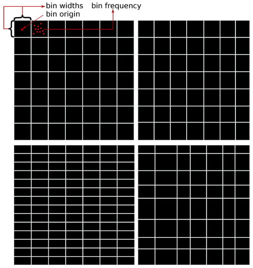
Figure 1. Examples of different grid scenarios in two dimensions. Upper left plot: each bin has an equal bin width $\mathit{h}=\{h,h\}$ with equal sides of bin h and an equal number of partitions in each dimension $\mathit{v}=\{v,v\}$. Upper right plot: each bin has an equal bin width $\mathit{h}=\{h_1,h_2\}$ with non equal sides of the bin $h_1\ne h_2$ and an equal number of partitions in each dimension $\mathit{v}=\{v,v\}$. Lower left plot: each bin has an equal bin width $\mathit{h}=\{h_1,h_2\}$ with non equal sides of bin $h_1\ne h_2$ and a non equal number of partitions in each dimension $\mathit{v}=\{v_1,v_2\}$. Lower right plot: each bin has a different bin width ${\mathit{h}}_j=\{h_{1j},h_{2j}\}$ with a different number of partitions in each dimension $\mathit{v}=\{v_1,v_2\}$.

Let ${\overline{\mathit{y}}}_1=\{{\overline{y}}_{11},\dots ,{\overline{y}}_{d1}\}$ be the first bin origin in the histogram grid. Let ${\mathit{h}}_1=\{h_{11},\dots ,h_{d1}\}$ be the first bin width. Each consecutive bin has the following bin origin

$${\overline{y}}_{ij}={\overline{y}}_{i1}+\frac{h_{i1}}{2}+\sum _{k=2}^{j-1}{h}_{ki}+\frac{h_{ij}}{2}\forall i\in \{1,\dots ,d\}.$$

(9)

Obviously, the histogram grid is defined by the first bin origin ${\overline{\mathit{y}}}_1$ and each histogram bin width ${\mathit{h}}_j$. It is usually taken that the first bin origin ${\overline{\mathit{y}}}_1={\mathit{y}}_{min}+{\mathit{h}}_1/2=\{y_{1min}+h_{11}/2,\dots ,y_{dmin}+h_{d1}/2\}$, where ${\mathit{y}}_{min}$ is a vector of the smallest component values from the dataset $\mathit{Y}$. Additionally, the histogram grid is constructed so that all the observations from the dataset $\mathit{Y}$ are contained. Usually, that is made by ensuring that the last bin origin ${\overline{\mathit{y}}}_V={\mathit{y}}_{max}-{\mathit{h}}_V/2=\{y_{1max}-h_{1V}/2,\dots ,y_{dmax}-h_{dV}/2\}$, where ${\mathit{y}}_{max}$ is a vector of the largest component values from the dataset $\mathit{Y}$. Finally, the $\mathit{y}\in V_j$ operation from Equation (8) is defined as

$$\mathit{y}\in V_j={\overline{y}}_{ij}-\frac{h_{ij}}{2}\le y_i<{\overline{y}}_{ij}+\frac{h_{ij}}{2}\forall i\in \{1,\dots ,d\},$$

(10)

and the observation ${\mathit{y}}_{max}$ is counted into last bin V. Let $k_j$ be the frequency of the jth bin. The frequency $k_j$ defines how many observations the jth bin holds. For the dataset $\mathit{Y}$ it is defined as

$$k_j\left(\mathit{Y}\right)=\sum _{j=1}^n{b}_j\left({\mathit{y}}_j\right).$$

(11)

The jth bin in the histogram grid consisting of V regular non-overlapping bins is thus defined with its origin ${\overline{\mathit{y}}}_j$, bin widths ${\mathit{h}}_j$ and empirical frequency $k_j$. Let the variable ${\mathit{x}}_j\in {\mathbb{R}}^{2d+1}$ uniquely define the jth bin. Then

$${\mathit{x}}_j=\{{\overline{\mathit{y}}}_j,{\mathit{h}}_j,k_j\}=\{{\overline{y}}_{1j},\dots ,{\overline{y}}_{dj},h_1,\dots ,h_d,k_j\}.$$

(12)

Remark 5.

In essence, the histogram grid is the tessellation of the d-dimensional Euclidean space. Apart from hyper-rectangles, any other polytope can be used as a tile. For example, in two-dimensional space, hexagons are often used. Nonetheless, obtaining a non overlapping grid with no gaps using other polytopes is not an easy job; hence, hyper-rectangles are the most preferred option. However, if used, the counting method remains the same; i.e., Equations (8) and (11) are unchanged; only the definition of operation $\mathit{y}\in V_j$ in Equation (10) is changed due to the different definition of the jth bin volume $V_j$.

To summarize, let $\mathit{X}=\{{\mathit{x}}_1,\dots ,{\mathit{x}}_V\}$ be the resulting matrix of the histogram estimation with V regular non-overlapping bins. Let $\mathit{H}=\{{\mathit{h}}_1,\dots ,{\mathit{h}}_V\}$ be the matrix of each bin width. The histogram estimation can then be summarized using

$$\mathit{X}=h\left(\mathit{Y}\right|\mathit{H})=\left\{\{{\overline{\mathit{y}}}_j,{\mathit{h}}_j,k_j\left(\mathit{Y}\right)\}\right|\forall j\in \{1,\dots ,V\}\}.$$

(13)

Remark 6.

A histogram estimation is not the same as histogram preprocessing, used for the preprocessing step in Algorithm 4. Although the above definition holds, the preprocessing step in Algorithm 4 removes all the empty bins—in other words, bins that have the frequency $k_j=0$—and the $\mathit{X}$ holds only bins for which $k_j>0$. Therefore, only the non-empty bins are left in the $\mathit{X}$. The number of non-empty bins $v^{*}$ is always $v^{*}\le V$. Additionally, for the dataset $\mathit{Y}$ with n observations, the number of non-empty bins is always $v^{*}\le n$.

3.1. Estimation of Optimum Histogram-Bin Widths

The main problem is estimating the number of bins V and the bin widths ${\mathit{h}}_j$ for each bin $j\in \{1,\dots ,V\}$. Most of the time an equal bin width for each and every bin can be safely assumed [22]; i.e.,

$${\mathit{h}}_1={\mathit{h}}_2=\dots ={\mathit{h}}_j=\dots ={\mathit{h}}_V=\{h_1,\dots ,h_i,\dots ,h_d\}.$$

(14)

Nonetheless, it should be pointed out that there is a lot of research on variable-bin-width, non-parametric density estimators [23], such as the histograms are themselves [22]. Thus, the jth bin’s origin, from Equation (9), becomes

$${\overline{y}}_{ij}={\overline{y}}_{i1}+(j-1)h_{i}i\in \{1,2,\dots ,d\},$$

(15)

and the first bin’s origin ${\overline{\mathit{y}}}_1$ can be safely estimated with

$${\overline{y}}_{i1}=y_{imin}+\frac{h_i}{2}i\in \{1,2,\dots ,d\}.$$

(16)

If the origin of the last bin is

$${\overline{y}}_{iV}=y_{imax}-\frac{h_i}{2}i\in \{1,2,\dots ,d\},$$

(17)

then the histogram-bin widths can be estimated as

$$h_i=\frac{y_{imax}-y_{imin}}{v_i}i\in \{1,2,\dots ,d\},$$

(18)

where $v_i\in \mathbb{Z}\wedge v_i\ge 1$ is the number of cuts in the ith dimension, which we referred to as the marginal number of bins in Section 2.4. In Algorithm 4 it is assumed that $v_1=v_2=\dots =v_i=\dots =v_d=v$, thereby making sure the loop in line 3 executes only $v_{max}-v_{min}+1$ times. Although this restriction seems strong, it often does not lead to a large deterioration in the estimates, especially after the EM algorithm’s utilization. Imagine, however, that this restriction is removed, and the set $K=\{v_{min},\dots ,v_{max}\}$ is applied to each $v_i\in \{v_1,\dots ,v_d\}$. This would lead to ${(v_{max}-v_{min}+1)}^d$ possible combinations and hence many loop executions. It is hard to find any practical example of when this large increase in execution times would be justified. Nevertheless, we ask ourselves whether, if the $\mathit{v}=\{v_1,v_2,\dots ,v_d\}$ can be inexpensively estimated, it could it result in improvements in the performance of the parameter estimation.

It is clear that the estimation of the histogram-bin width $\mathit{h}$, as described above, can be translated into an estimation of the histogram’s number of bins $\mathit{v}$. In the following explanations we will refer to the different number of bins $\mathit{v}$ as different binning $\mathit{v}$ and the histogram estimation for the binning $\mathit{v}$ is the problem of estimating the frequency $k_j$ for each bin j, as defined in Equation (11). The problem of estimating the optimum binning $\mathit{v}$ can thus be formulated as the following constrained-integer optimization problem

$$maxH\left(\mathit{v}\right),$$

(19)

where $\mathit{v}=\{v_1,\dots ,v_d\}\in {\mathbb{Z}}^d\wedge v_i\ge 1\forall v_i\in \mathit{v}$ and $H\left(\mathit{v}\right)$ is the optimization function that calculates the goodness of the histogram estimation with binning $\mathit{v}$. Generally speaking, as was already stated in [24], this is an NP-hard problem, which cannot be solved in polynomial time. Additionally, most of the approaches for solving the integer-optimization problem usually remove the integer constraint and solve the equivalent real-valued problem [24]. As the evaluation of the optimization function $H\left(\mathit{v}\right)$ requires the histogram estimation, finding the optimum binning $\mathit{v}$, by removing the integer constraint, and for example, using the gradient methods, is not favorable, since the derivatives of the above-presented histogram estimation and consequently the optimization function $H\left(\mathit{v}\right)$ need to be numerically estimated. Hence, the optimization method will require multiple repetitions of the histogram estimations with different numbers of bins $\mathit{v}$ and consequently evaluations of the function $H\left(\mathit{v}\right)$. To ease the optimization problem slightly, we will also adopt another constraint in the form of the maximum marginal number of bins $v_{max}$ and the minimum marginal number of bins $v_{min}$, so that

$$v_{min}\le v_i\le v_{max}\forall v_i\in \mathit{v}$$

(20)

holds. As the most straightforward implementation, which we will refer to as exhaustive search, would be to evaluate the optimization function $H\left(\mathit{v}\right)$ for each and every binning $\mathit{v}$ from the set

$$C=K\times K\dots K=K^d=\{\{v_1,\dots ,v_i,\dots ,v_d\}\mid v_i\in K\forall i\in \{1,\dots ,d\}\},$$

(21)

which is in fact the d-ary Cartesian product of set $K=\{v_{min},v_{min}+1,\dots ,v_{max}\}$.

The algorithm implementation is presented in Algorithm 5. As was already stated, the evaluation of the function $H\left(\mathit{v}\right)$ requires a histogram estimation with binning $\mathit{v}$, which can be made in $O\left(n\right)$, where n is the number of observations in the input dataset $\mathit{Y}$, so it can be assumed that the efficient implementation of the $H\left(\mathit{v}\right)$ estimation can be made in $O\left(n\right)$. However, the number of candidates in the constructed set C, from line 2 of Algorithm 5 is ${(v_{max}-v_{min}+1)}^d$. If $v_{min}=1$ and $v_{max}=n$ are assumed, the computational complexity of Algorithm 5 becomes $O\left(n^{d+1}\right)$, which is definitely not desirable as the datasets with large numbers of dimensions are now quite common [25]. However, if the set C contains the optimum candidate, that value would be selected.

Algorithm 5: Exhaustive search for optimum histogram binning $\mathit{v}$.

1:  Input dataset $\mathit{Y}$, initialize set $K=\{v_{\min },v_{\min }+1,\dots ,v_{\max }\}$; 2:  Construct set $C=K^d$ with Equation (21); 3:  Set ${\widehat{H}}_{\mathrm{opt}}=-\infty$, ${\mathit{v}}_{\mathrm{opt}}=\left\{\right\}$; 4:  foreach $\mathit{v}\in C$ do: 5:    Evaluate $\widehat{H}=H\left(\mathit{v}\right)$; 6:    if $\widehat{H}>{\widehat{H}}_{\mathrm{opt}}$: 7:       ${\widehat{H}}_{\mathrm{opt}}=\widehat{H}$, ${\mathit{v}}_{\mathrm{opt}}=\mathit{v}$; 8:    end 9:  end

To solve the above problem more efficiently than with the exhaustive search, we used the derivation of the coordinate-descent optimization algorithm. The coordinate descent and its variants are types of hill-climbing optimization algorithms [26]. Hence, given some initial starting value of the optimized parameters, it will always choose local optima, given that the optimization function is not convex. The solution is obtained by cyclically switching the coordinates, i.e., the dimensions, of the optimization problem. For each dimension it searches for the optimum value of the parameter in that dimension, while keeping other parameter values (in other dimensions) constant. As it finishes it moves to the next dimension and repeats the process until convergence. The search for the optimum parameter value in each dimension can be made by calculating the gradient or using a line search. Given that we already stated that a line search is preferred over a gradient calculation, the algorithm implementation is given in Algorithm 6.

Algorithm 6: Coordinate-descent algorithm for optimum histogram binning $\mathit{v}$.

1:  Input dataset $\mathit{Y}$, initialize set $K=\{v_{\min },v_{\min }+1,\dots ,v_{\max }\}$; 2:  Set ${\widehat{H}}_{\mathrm{opt}}=-\infty$, $v_{\mathrm{opt}}=0$, ${\mathit{v}}_{\mathrm{opt}}=\left\{\right\}$; 3:  Set initial starting position $\mathit{v}=\{v_1,\dots ,v_i,\dots ,v_d\}$ so that $v_1=\dots =v_i=\dots =v_d=1$; 4:  Set Converged = False; 5:  while Converged is not True do: 6:    foreach $i\in \{1,\dots ,d\}$ do: 7:       Set $v_{i\mathrm{old}}=v_i$, $v_{\mathrm{opt}}=v_{i\mathrm{old}}$; 8:       foreach $v\in K$ do: 9:          Update $v_i\in \mathit{v}$ so that $v_i=v$; 10:          Evaluate $\widehat{H}=H\left(\mathit{v}\right)$; 11:          if $\widehat{H}>{\widehat{H}}_{\mathrm{opt}}$: 12:             ${\widehat{H}}_{\mathrm{opt}}=\widehat{H}$, $v_{\mathrm{opt}}=v$, ${\mathit{v}}_{\mathrm{opt}}=\mathit{v}$; 13:          end 14:       end 15:       if $i=1\wedge v_{\mathrm{opt}}=v_{i\mathrm{old}}$: 16:          Set Converged = True; 17:       end 18:    end 19:  end

Essentially, as stated above, in each dimension i, the marginal number of bins $v_i$ is optimized by performing a line search from the supplied minimum value $v_{min}$ to the maximum value $v_{max}$ for a fixed step size of 1 (construction of the ordered set K). When estimating the optimum parameter value of $v_i$, other parameter values are kept constant (in other dimensions). The parameter values for the other dimensions (ones which are not currently being estimated) are obtained from a previously conducted line search or using the starting initial value of $\mathit{v}$. The convergence is assessed as follows. The number of iterations I of the Algorithm 6 are counted by the number of while-loop (lines 5–19 of Algorithm 6) executions. Each iteration of the while loop starts by updating the parameter value in the first dimension of the problem; i.e., $i=1$ and $v_i=v_1$. Hence, if this parameter value has not changed, it is an obvious clue that in other dimensions the parameter values will not change, given that at least one iteration of Algorithm 6 has passed; i.e., $I>1$. To ensure that Algorithm 6 will perform at least one iteration, i.e., the condition $I>1$, we chose to hard code the initial starting-parameter values to 1 (line 3 of Algorithm 6). This is clearly unwanted binning $\mathit{v}$ as it results in only one bin; hence, the estimated value ${\widehat{H}}_{\mathrm{opt}}$ of the optimization function $H\left(\mathit{v}\right)$ can be safely set to the worst value; e.g., in the maximization case ${\widehat{H}}_{\mathrm{opt}}=-\infty$.

It is hard to predict the necessary number of iterations I for the convergence of Algorithm 6, as it depends on the input dataset $\mathit{Y}$. With an increase in the number of iterations I, the number of optimization-function $H\left(\mathit{v}\right)$ evaluations increases. In the worst-case scenario, the number of $H\left(\mathit{v}\right)$ evaluations can even surpass the number of evaluations in the exhaustive search variant given in Algorithm 5, due to the fact that the same value of $\mathit{v}$ could be revisited in the optimization procedure. As the optimization function $H\left(\mathit{v}\right)$ evaluation is the computationally most burdening part of Algorithm 6, this is clearly unwanted. However, to set the upper limit of the $H\left(\mathit{v}\right)$ evaluations to be equal to the number of evaluations in the exhaustive search variant (Algorithm 5), we have used a simple memoization technique [27]. Memoization is often used in dynamic programming and recently also to improve the performance of metaheuristic algorithms [28]; however, it should be noted that it leads to an increase in memory usage. However, as pointed out in [28], it is hard to imagine this as an issue, given that the advances in hardware technology lead to massive capacities of inexpensive memory. The memoized version of the coordinate-descent algorithm for optimum histogram binning $\mathit{v}$ is given in Algorithm 7.

Algorithm 7: Coordinate-descent algorithm for optimum histogram binning $\mathit{v}$ with memoization.

1:  Input dataset $\mathit{Y}$, initialize set $K=\{v_{\min },v_{\min }+1,\dots ,v_{\max }\}$; 2:  Set ${\widehat{H}}_{\mathrm{opt}}=-\infty$, $v_{\mathrm{opt}}=0$, ${\mathit{v}}_{\mathrm{opt}}=\left\{\right\}$; 3:  Set initial starting position $\mathit{v}=\{v_1,\dots ,v_i,\dots ,v_d\}$ so that $v_1=\dots =v_i=\dots =v_d=1$; 4:  Initialize memoization dictionary $D=\left\{\right\}$; 5:  Set Converged = False; 6:  while Converged is not True do: 7:    foreach $i\in \{1,\dots ,d\}$ do: 8:       Set $v_{i\mathrm{old}}=v_i$, $v_{\mathrm{opt}}=v_{i\mathrm{old}}$; 9:       foreach $v\in K$ do: 10:          Update $v_i\in \mathit{v}$ so that $v_i=v$; 11:          if $H\left(\mathit{v}\right)$ already evaluated and stored in dictionary D: 12:             Retrieve stored value of $\widehat{H}$ stored for value $\mathit{v}$; 13:          else: 14:             Evaluate $\widehat{H}=H\left(\mathit{v}\right)$; 15:             Store value $\widehat{H}$ in dictionary D for $\mathit{v}$; 16:          end 17:          if $\widehat{H}>{\widehat{H}}_{\mathrm{opt}}$: 18:             ${\widehat{H}}_{\mathrm{opt}}=\widehat{H}$, $v_{\mathrm{opt}}=v$, ${\mathit{v}}_{\mathrm{opt}}=\mathit{v}$; 19:          end 20:       end 21:       if $i=1\wedge v_{\mathrm{opt}}=v_{i\mathrm{old}}$: 22:          Set Converged = True; 23:       end 24:    end 25:  end

The intuition behind using the coordinate-descent algorithm for our optimization purposes comes from the histogram estimation being the most trivial non-parametric probability density estimator [29]. Most of the time it is used on a univariate (one-dimensional) random variable; however, as in our case, it can be used for a multivariate (multidimensional) random variable. If, for example, we assume independence between each dimension in a random variable $\mathit{y}\in {\mathbb{R}}^d$, the problem of estimating each $v_i\in \mathit{v}$ could be broken in d univariate problems, and the estimation of each marginal number of bins $v_i$ could be conducted separately. This could result in a large overestimation of each marginal number of bins $v_i$, due to the fact that in a d-dimensional problem the actual number of bins in the histogram grid is $V={\prod }_{i=1}^d{v}_i$. Given that a larger number of bins leads to more empty bins in the histogram grid (e.g., when $V>>n$), most of the $H\left(\mathit{v}\right)$ will penalize such a solution. When using the coordinate-descent algorithm, we act analogously; however, we do so by taking into account the actual number of bins in the d-dimensional grid. Nonetheless, as already stated, the coordinate-descent algorithm can be trapped into some spurious local optima. To ensure that the best possible solution is estimated, we use the results from the coordinate-descent algorithm to conduct an exhaustive search in a narrowed parameter space, as shown in Algorithm 8. To clarify why this could be helpful, let us imagine the following scenario. Let some marginal number of bins $v_i$ be underestimated, whereas some other marginal number of bins $v_{\tilde{ı}}$ is overestimated (e.g., in some dimension i, the estimated value of $v_i$ is smaller than the optimum, and in some other dimension $\tilde{ı}\ne i$, the estimated parameter of the value $v_{\tilde{ı}}$ is higher than the optimum). A new set K can be constructed from the minimum estimated value to the maximum estimated value, as shown in lines 3 and 4 of Algorithm 8 and constructing all the possible combinations from the set K (constructing the set C from line 5 of Algorithm 8) will ensure that the optimum solution is acquired. Although there is no clear evidence that the utilization of an additional exhaustive search will be beneficial, we presume that the newly constructed set K and consequently set C (line 5 and 6 of Algorithm 8) will hold many fewer candidates for the optimum solution. Additionally, due to using the memoization technique, a lot of possible solutions are already visited; thus, an additional exhaustive search should not lead to an exceptional increase in the computational time.

Algorithm 8: Narrowed exhaustive search with a coordinate-descent algorithm for optimum histogram binning $\mathit{v}$ with memoization.

1:  Input dataset $\mathit{Y}$, initialize set $K=\{v_{\min },v_{\min }+1,\dots ,v_{\max }\}$; 2:  Obtain ${\mathit{v}}_{\mathrm{opt}}$ using Algorithm 7; 3:  Set $v_{min}=min\left({\mathit{v}}_{o}pt\right)$; 4:  Set $v_{max}=max\left({\mathit{v}}_{o}pt\right)$; 5:  Construct narrowed set $K=\{v_{\min },v_{\min }+1,\dots ,v_{\max }\}$; 6:  Construct set $C=K^d$ with Equation (21); 7:  foreach $\mathit{v}\in C$ do: 8:    if $H\left(\mathit{v}\right)$ already evaluated and stored in dictionary D: 9:       Retrieve stored value of $\widehat{H}$ stored for value $\mathit{v}$; 10:    else: 11:       Evaluate $\widehat{H}=H\left(\mathit{v}\right)$; 12:       Store value $\widehat{H}$ in dictionary D for $\mathit{v}$; 13:    end 14:    if $\widehat{H}>{\widehat{H}}_{\mathrm{opt}}$: 15:       ${\widehat{H}}_{\mathrm{opt}}=\widehat{H}$, ${\mathit{v}}_{\mathrm{opt}}=\mathit{v}$; 16:    end 17:  end

3.2. The Knuth Rule as the Optimization Function

Finally, let us address the elephant in the room; i.e., the optimization function $H\left(\mathit{v}\right)$. For the optimization function $H\left(\mathit{v}\right)$ the Knuth rule defined in [22] is used. The Knuth rule yielded good estimates when used in [4], and additionally, due to its usability in a multivariate setting, it was chosen here. The Knuth rule is defined as

$$H\left(\mathit{v}\right)=nlogV+log\Gamma \left(\frac{V}{2}\right)-Vlog\Gamma \left(\frac{1}{2}\right)-log\Gamma (n+\frac{1}{2})+\sum _{j=1}^{V}log\Gamma (k_j\left(\mathit{Y}\right)+\frac{1}{2})+const,$$

(22)

where $\mathit{Y}$ is the dataset, n is the number of observations in the dataset, V is the number of bins, $log\Gamma$ is the natural logarithm of the gamma function and $const$ is an integration constant. It is clear that different binning $\mathit{v}$ should produce different results for $H\left(\mathit{v}\right)$, even though it is not obvious from the definition in Equation (22). Different binning $\mathit{v}$ leads to different frequencies $k_j\left(\mathit{Y}\right)$, if we recall Equation (11), and additionally, a different number of bins V, ultimately giving different values to the ${\sum }_{j=1}^{V}log\Gamma (k_j\left(\mathit{Y}\right)+1/2)$ term in Equation (22). Nonetheless, as the number of bins V increases (with the increase in the marginal number of bins $v_i$, the bin width shrinks $h_i\to 0$), it will lead to the state where each populated bin contains only one observation, $k_j\left(\mathit{Y}\right)=1\forall j\in \{1,\dots ,n\}$ and the rest of the bins will have a frequency of zero. Since computers digitize the data, as was stated in [22], this is a most unlikely scenario for every dataset $\mathit{Y}$; however, after passing some final binning ${\mathit{v}}_{\mathrm{final}}$, as the order of the bins in Equation (22) is not important, the term ${\sum }_{j=1}^{V}log\Gamma (k_j\left(\mathit{Y}\right)+1/2)$ will not change and the change of $H\left(\mathit{v}\right)$ will be dependent on the number of bins V. If we assume that for the final binning $v_{\mathrm{final}}$ we have the scenario where each populated bin holds one observation, Equation (22) transforms into

$$H\left(V\right)=nlogV+log\Gamma \left(\frac{V}{2}\right)-log\Gamma (n+\frac{1}{2})+nlog\Gamma (1+\frac{1}{2})-nlog\Gamma \left(\frac{1}{2}\right)+const.$$

(23)

The value of $H\left(V\right)$ from Equation (23) is monotonically increasing as V increases. This could jeopardize the estimation process for the optimum solution $\mathit{v}$ in Algorithm 8. Therefore, to determine when the evaluation of the Knuth rule (Equation (22)) is no longer usable, due to this possible degeneration, we have chosen to constrain the maximum number of non-empty bins $v_{max}^{*}$ in the histogram grid; in other words

$$v_{max}^{*}=\frac{1+d}{d}{n}^{\frac{d}{1+d}}.$$

(24)

The Equation (24) for $d=1$ yields the famous RootN rule $v_{max}^{*}=2\sqrt{n}$ and as the dimension increases $d\to \infty$ the limiting number of populated bins is $v_{max}^{*}\to n$. Hence, after each histogram estimation the number of non-empty bins in the histogram grid is checked and if the number of non-empty bins $v^{*}$ is higher than $v_{max}^{*}$, then the solution is rejected.

Remark 7.

Although the $v_{max}^{*}$ should be an integer, the result of Equation (24) is real; i.e., $v_{max}^{*}\in \mathbb{R}$. Since the $v_{max}^{*}$ is only used for comparison, the need to be an integer is thus avoided.

4. Experiments

Two experiments were conducted to evaluate our proposals. For the first experiment, we simulated different datasets to evaluate the proposed algorithm for estimating the optimum histogram binning $\mathit{v}$ in conjunction with the Knuth rule as the optimization function. Datasets were simulated for $d=2$, $d=3$ and $d=4$ numbers of dimensions. Simulations of the datasets were made in the following manner. A random number of observations was drawn uniformly on a unit hypercube in ${\mathbb{R}}^d$ (length of each side was set to $h=1$). The number of observations to sample on each unit hypercube was drawn from a uniform distribution on the (10, 100) interval. The number of unit hypercubes was determined by the marginal number of bins $v_i$ in each dimension. For the $d=2$, we have chosen $v_1=7$; $v_2=10$ for the $d=3$ we chose $v_1=8,v_2=6,v_3=4$; and for $d=4$ we chose $v_1=4,v_2=7,v_3=3,v_4=5$. Thus, for $d=2$ we had $V=70$ hypercubes, for $d=3$ we had $V=192$ and for $d=4$ we had $V=420$. To additionally increase the difficulty of the estimation process, we have chosen to leave some bins empty, i.e., the number of observations in some unit hypercubes was set to 0. Empty bins were also determined randomly; however, as the number empty bins increases, the problem becomes harder, and we have given a larger probability to an empty bin than for a populated bin. As the number of bins increased with the increase in the number of dimensions d, the probability of an empty bin was increased for each dimension, so in $d=2$ we used 0.75; in $d=3$ the probability of an empty bin was increased to 0.85; and for $d=4$ it was 0.95. Finally, for each dimension d we simulated 100 different datasets with a different seed number for a random generator. Examples of ten simulated datasets for $d=2$ are shown in Figure 2. To estimate the optimum binning $\mathit{v}$ with the Knuth rule we chose the following strategies. To ensure the best solution, at least when using the Knuth rule, is selected, we used the exhaustive strategy with $v_{min}=2$ and $v_{max}=100$, and refer to this as EXHOPTBINS. The second strategy was the proposed coordinate-descent algorithm implementation in Algorithm 8 with $v_{min}=2$ and $v_{max}=100$. This was referred to as OPTBINS. Additionally, some commonly used metaheuristic algorithms, the genetic algorithm and simulated annealing, were used. For the genetic algorithm we used the GA R package [30,31] and for the simulated annealing we used the optimization R package [32]. In what follows, the genetic algorithm is referred to as the GA, and simulated annealing as SA. For the GA and SA algorithms, $v_{min}=2$ and $v_{max}=100$ were also set. For other parameters for GA and SA, default values were used for corresponding R packages. Additionally, to ensure fair comparisons, we added the memoization principle in the GA and SA software implementation, so that only for newly visited parameter $\mathit{v}$ was the histogram evaluated.

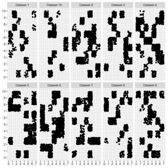
Figure 2. Simulated datasets for the first experiment.

In the second experiment we wanted to evaluate how the estimation of the optimum binning ${\mathit{v}}_{\mathrm{opt}}$ affects the estimation of the Gaussian mixture-model parameters with the REBMIX&EM methodology. For testing purposes we used four different datasets, all having different difficulties in the estimation of the Gaussian mixture-model parameters. For the comparison we used the exhaustive REBMIX&EM strategy with $v_{min}=2$ and $v_{max}=100$, the best REBMIX&EM strategy with $v_{min}=2$ and $v_{max}=100$ and the two single REBMIX&EM strategies with the Knuth rule estimated using an equal marginal number of bins $v_1=\dots =v_d=v$ and an unequal marginal number of bins estimated using the proposed algorithm. The estimated optimum binning ${\mathit{v}}_{opt}$ with the proposal used to start the single REBMIX&EM strategy to estimate the parameters of the Gaussian mixture model is referred to as the single REBMIX&EM with NK. The Knuth rule used in [4] with an equal marginal number of bins $v_1=\dots =v_d=v$ is referred to as the single REBMIX&EM with EK. For the estimation of the optimum binning for both scenarios we used the same setting; i.e., $v_{min}=2$ and $v_{max}=100$. Additionally, for a sanity check we added the optimum Gaussian mixture-model parameters estimated with the mclust R package [21]. To ensure fair comparisons, we used only the most general VVV model from the mclust package. For the information criterion, for model-selection purposes, the Bayesian information criterion (BIC) was used [33]. The minimum number of components $c_{min}$ was kept to 1 and the maximum number of components was set to $c_{max}=15$.

5. Results

5.1. First Experiment

The results for the first experiment are summarized in Table 1 and Table 2 and Figure 3. If we recall this experiment’s setting, described in Section 4, there were 100 different datasets for the dimensions $d=2$, $d=3$ and $d=4$. For each dimension d, the datasets were simulated from the known binning $\mathit{v}$ and replicated 100 times with different random settings. Hence, for the first useful insight, we evaluated on how many datasets for each dimension d, each algorithm used was capable of finding the true binning $\mathit{v}$ from which the dataset was simulated. The results were given in Table 1. It is clear that the EXHOPTBINS and OPTBINS algorithms had true solutions on most of the datasets—65. For the EXHOPTBINS algorithm this was expected; however, it seems that the OPTBINS algorithm was clearly capable of selecting the same solution as EXHOPTBINS. Moving forward, the GA and SA algorithms had a true solution on a slightly smaller number of datasets than the EXHOPTBINS/OPTBINS algorithms. For the datasets with $d=3$ and $d=4$ m we could not evaluate the EXHOPTBINS algorithm, as the time spent on only one dataset was a couple of hours, which would ultimately make EXHOPTBINS run in a couple of days, which was not acceptable. However, other algorithms were successful and even better than on $d=2$ datasets. The OPTBINS and GA algorithms had true solutions on more datasets than they had on $d=2$, while the SA algorithm had a small deterioration for $d=3$ and a larger deterioration for $d=4$.

Table 1. Number of datasets with true binning $\mathit{v}$ selected for each dimension of the dataset d.

Dimension d of Dataset	OPTBINS	EXHOPTBINS	GA	SA
$d=2$	65/100	65/100	62/100	64/100
$d=3$	95/100	*	90/100	61/100
$d=4$	91/100	*	71/100	29/100

Table 2. Number of datasets for the $d=2$ with equal binning $\mathit{v}$ selected as the EXHOPTBINS algorithm.

Algorithm	Number of Datasets
OPTBINS	100/100
GA	95/100
SA	98/100

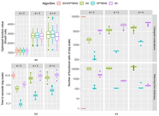
Figure 3. Results obtained from the first experiment: (a) Optimization-function value—the Knuth rule defined in Equation (22), for each algorithm and dimension of the dataset d. (b) Time spent for each algorithm to obtain optimum binning ${\mathit{v}}_{\mathrm{opt}}$ for each dimension of the dataset d. (c) Number of true function evaluation calls; i.e., histogram evaluations vs. the number of silent function evaluation calls; i.e., retrieving the stored value from memoization dictionary for each algorithm and dimension of the dataset d.

The true solution was not selected for almost one-third of the datasets in $d=2$. However, as we saw, even the exhaustive search EXHOPTBINS algorithm was also unable to find the true solution, so it can only be said that the Knuth rule optimization function preferred some other binning scenario as the optimum for the mentioned datasets. Nonetheless, as the solution given by EXHOPTBINS can be seen as ultimately the best solution possible for the given range of $v_{min}=2$ and $v_{max}=100$, Table 2 gives the number of datasets on which the algorithms OPTBINS, GA and SA gave the same solution as EXHOPTBINS. As expected, the results were relatively good, making the Knuth rule an obviously simple function for each of the three chosen optimization procedures.

Finally, the box-plots given in Figure 3 provide some overview of the computational costs needed for each of the optimization algorithms employed. First, to confirm the results presented in Table 1 and Table 2 we have given the box-plots of the optimum function values, i.e., the values of the Knuth rule from Equation (22), in plot a of Figure 3. As can be seen, the optimization-function values for each dimension d of the dataset are equal, confirming the results presented before, i.e., most of the time all the algorithms selected the same optimum binning $v_{\mathrm{opt}}$. Next, we gave both the computational times (plot b) of Figure 3 and the number of optimization-function evaluations (plot c) of Figure 3 for each algorithm and each dimension d of the simulated dataset. We added both plots to ensure fairer comparisons, as the computational times can be affected by the algorithm implementations and the programming language used. It is clear from plot b of the Figure 3 that the OPTBINS algorithm had many the shortest computational times. On other hand, the GA and SA algorithms had almost the same computational times. On plot c of Figure 3 we added two graphs, the upper giving the optimization-function evaluations, including the histogram estimations, which are the most wasteful, and the lower graph, giving only the number of calls to the shared dictionary from which the optimization-function value was retrieved in the case of the already-visited solutions. For the OPTBINS algorithm we can see that most of the calls were made on newly visited solutions; however, the number of optimization-function evaluations was the smallest. On other hand, both the GA and SA had many more optimization-function evaluations. In the end, as we can see, the number of times the GA algorithm revisited already visited solutions was exceptionally high; hence, the application of the memoization trick to the GA was definitely beneficial, whereas in the case of the SA the number of revisits was reducing with the dimension d, thereby implying the reduced benefit of the memoization trick.

5.2. Second Experiment

For the purposes of a comparison, in the second experiment we used the value of the model goodness-of-fit estimator; i.e., the information criterion value (BIC). Additionally, the simulated datasets and real-world datasets used can be seen as a clustering problem. All the observations from the datasets have their cluster membership known. On other hand, in the Gaussian mixture-model ecosystem, the components are usually receipted as clusters [14]. In other words, by using the posterior probabilities we can label the observations from the dataset in the maximum a-posterior fashion. Each observation corresponds to a component/cluster of a Gaussian mixture model for which it yielded the maximum posterior probability. Hence, the clustering performance of each estimated Gaussian mixture-model parameter can be evaluated. To evaluate the clustering performance, the adjusted Rand index (ARI) was used [34]. Additionally, to evaluate the computational intensity, the elapsed time for each method was used together with the number of EM iterations needed to complete the estimation process. As the mclust implementation does not offer the number of EM iterations as an output parameter, we reported only the computation time.

5.2.1. Simulated Dataset with a Small Level of Overlap between the Clusters

In this example we used the MixSim R package [35] to simulate the parameters of the Gaussian mixture model in ${\mathbb{R}}^2$, where the overlap between the Gaussian mixture-model components is relatively small. The number of components c was set to five. The parameters are used to simulate the dataset from the obtained parameters of the Gaussian mixture model. The simulated dataset is shown in Figure 4. The number of observations n in the dataset was set to 1000.

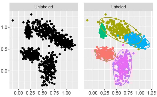
Figure 4. Simulated dataset with low overlapping clusters.

The results are presented in Table 3 and Figure 5. Table 3 gives some numerical results, while Figure 5 gives a graphical representation of the estimated Gaussian mixture-model parameters and clustering solutions. From Table 3 it is clear that all the strategies used estimated almost identical parameters for the Gaussian mixture model (the value of BIC is almost identical and the number of components c is the same along with the clustering performance). This can also be confirmed by observing Figure 5. However, for the last two columns of Table 3 it is clear that some strategies did take a longer time to estimate the parameters and more of the expensive EM algorithm iterations, while the other was shorter and with a smaller number of EM algorithm iterations. First, the exhaustive REBMIX&EM strategy needed a very large number of EM iterations, and therefore, an unjustifiable amount of computational time. On other hand, the best REBMIX&EM strategy needed more time for the REBMIX algorithm (0.138 s) than estimating the optimum binning ${\mathit{v}}_{\mathrm{opt}}$ for both the single REBMIX&EM strategies (for the OPTBINS algorithm the required time was 0.017 s and for the Knuth rule with an equal marginal number of bins, 0.004 s). However, the initial estimates with the best REBMIX&EM of the Gaussian mixture-model parameters needed a smaller number of more expensive EM iterations with the best REBMIX&EM strategy than the single REBMIX&EM strategy with EK. Ultimately, this led to a faster estimation of the Gaussian mixture-model parameters with the best REBMIX&EM strategy than with the single REBMIX&EM strategy with EK. On other hand, as we already stated, the estimation of the optimum binning ${\mathit{v}}_{\mathrm{opt}}$ with the proposed OPTBINS algorithm was faster than estimating the REBMIX algorithm for different binning $\mathit{v}$, and additionally led to the smaller number of EM iterations needed for the convergence criteria. Finally, the mclust strategy gave a solution in a reasonable and comparable amount of time.

Table 3. Results on the dataset with a low level of overlap between the clusters.

Strategy	c	BIC	ARI	Number of EM it Erations	Time [s]
Single REBMIX&EM with EK	5	−1145.142	0.896	2347	1.209
Single REBMIX&EM with NK	5	−1145.143	0.896	1874	1.044
Best REBMIX&EM	5	−1145.141	0.896	1970	1.081
Exhaustive REBMIX&EM	5	−1145.148	0.896	37,798	15.838
mclust	5	−1145.088	0.885	/	1.983

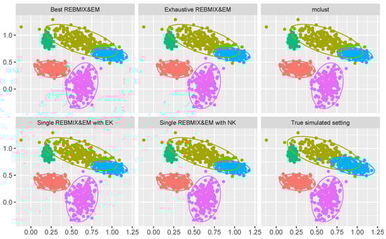
Figure 5. Solutions obtained from different methods used and the true clustering solution on the low overlapping clustering dataset.

5.2.2. Simulated Dataset with High Level of Overlap between the Clusters

For the second example we increased the difficulty of the problem. Again, we simulated the parameters of the Gaussian mixture model in ${\mathbb{R}}^2$ with the MixSim R package, except we increased the overlap level between the Gaussian mixture-model components. Again, the number of components was set to $c=5$ and the number of observations in the sampled dataset was $n=1000$. This example is shown in Figure 6.

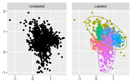
Figure 6. Simulated dataset with high overlapping clusters.

The results are given in Table 4 and Figure 7. Judging only by the BIC values and the estimated number of components c, the single REBMIX&EM strategy with EK had significantly poorer results than the other strategies concerning the quality of the Gaussian mixture parameter estimation. The single REBMIX&EM strategy with EK estimated the Gaussian mixture model with six components, which decreased the quality of the estimation. However, by inspecting Figure 7 it can be seen that only the exhaustive REBMIX&EM, single REBMIX&EM with EK and single REBMIX&EM with NK strategy had the best estimation of the mostly overlapping component in the Gaussian mixture model (the component that was colored yellow in Figure 7). The best REBMIX&EM strategy and mclust favored a smaller overlap between components. Additionally, only the single REBMIX&EM with the NK strategy had the best estimation of the blue component parameters. Thus, the value of ARI was higher than for the other strategies; however, not to any great extent. The value of ARI was not so convincingly high as in the previous case because of the large amount of overlap between the clusters in the simulated setting. As for the computational performance, the single REBMIX&EM with NK strategy had the smallest number of EM iterations and the shortest computational time. Again, the number of iterations and the estimation time for the exhaustive REBMIX&EM strategy was unadjustable, even though it had the second-best results and the best result obtained if compared to the BIC value (lower is better). The best REBMIX&EM strategy and mclust had good solutions with reasonable computation times. To conclude, even though the single REBMIX&EM strategy with EK estimated the Gaussian mixture model with six components, this solution is not poorer in terms of quality than the other solutions, as the estimation problem was hard.

Table 4. Results on the dataset with high level of overlap between clusters.

Strategy	c	BIC	ARI	Number of EM Iterations	Time [s]
Single REBMIX&EM with EK	6	1781.344	0.464	4860	2.285
Single REBMIX&EM with NK	5	1752.988	0.493	2460	1.122
Best REBMIX&EM	5	1759.069	0.460	3396	1.588
Exhaustive REBMIX&EM	5	1751.605	0.467	58,906	15.838
mclust	5	1759.246	0.461	/	2.970

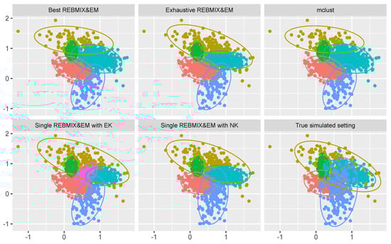
Figure 7. Solutions obtained from different methods used and the true clustering solution on a high overlapping clustering dataset.

5.2.3. Cross Dataset

This example was used from the study in [36]. The dataset was simulated in ${\mathbb{R}}^3$ and it gives two clusters of data, both of which belong to an object with a geometrical shape, cross and rectangular bar; see Figure 8. As the geometrical shape of a cross is impossible to recover within the Gaussian mixture-model clustering framework, the two-cluster solution would be inappropriate to use (the study in [36] was aiming to combine the mixture-model components in order to obtain such complicated clustering solutions). Hence, we adopted the three-cluster solution as ideal, which was also reported in [36] as one of the optimum Gaussian mixture models selected by the model-selection procedure with the BIC criterion in their study. For convenience, we added a top-down view of the dataset in Figure 9. This dataset increases the difficulty, as it has a substantial overlap between clusters, and additionally the dimension of the problem is higher. Furthermore, there were fewer observations in this dataset; i.e., $n=300$.

Figure 8. Cross dataset from [36]. The first plot gives the unlabeled observations; the second plot gives the true two-cluster clustering; and the third plot gives the ideal three-cluster clustering.

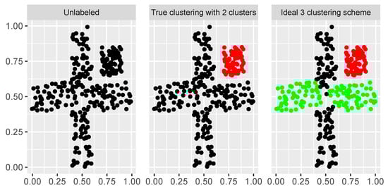
Figure 9. Top-down view of cross dataset from [36]. The first plot gives the unlabeled observations; the second plot gives the true two-cluster clustering; and the third plot gives the ideal three-cluster clustering.

The results can be found in Table 5 and Figure 10. The results in Figure 10 are shown for the top down view only, as they reveal the most information. As we can see, the single REBMIX&EM with NK and the best REBMIX&EM selected our preferable solution, and thus for their clustering partitioning the estimated ARI value was highest. Nonetheless, the parameters of the Gaussian mixture model estimated with the exhaustive REBMIX&EM strategy were good, as this solution was also reported in [36] as appropriate with BIC as the model-selection criterion. The solution obtained with the single REBMIX&EM with EK had five components/clusters, and the solution from the mclust had six components/clusters. We find this two-cluster solution to have a slightly poorer quality than the other solution; however, it was acceptable due to the obvious hardness of the problem. Comparing the computational expenses of using each of the selected strategies, it is clear that the single REBMIX&EM strategy with NK is the fastest, although it had more EM iterations than the single REBMIX&EM with EK. On other hand, again, the increase in the computational time for the exhaustive REBMIX&EM strategy was unjustified. The best REBMIX&EM strategy and the mclust had similar computational times.

Table 5. Results on the cross dataset from [36].

Method	c	BIC	ARI	Number of EM Iterations	Time [s]
Single REBMIX&EM with EK	5	−825.576	0.653	605	0.124
Single REBMIX&EM with NK	3	−855.274	0.967	906	0.098
Best REBMIX&EM	3	−855.274	0.967	1273	0.293
Exhaustive REBMIX&EM	4	−855.755	0.741	7217	1.091
mclust	6	−801.828	0.506	/	0.340

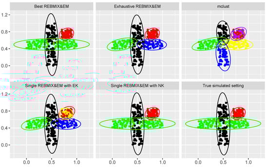
Figure 10. Solutions obtained with different methods used and the true clustering solution on a high overlapping clustering dataset.

5.2.4. Iris Dataset

As our final dataset we chose the real-world Iris dataset [37]. This is relatively famous and commonly used as a dataset for benchmarking classification algorithms and also in a mixture-model clustering framework. It consist of 150 measurements (observations) of four characteristics of Iris flowers. Three species of Iris flowers are measured: virginica, versicolor and setosa. The characteristics measured on each iris flower are sepal length, sepal width, petal length and petal width. In the classification framework, i.e., as a supervised learning task, this dataset is mostly taken as simple; however, in unsupervised learning, i.e., clustering, it can be quite hard to estimate the right number of clusters due to the overlap of the measurements between the virginica and versicolor species of iris flowers, Figure 11.

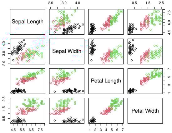
Figure 11. Iris dataset [37]. Black circles represent the setosa species of iris flower. The red circles are versicolor and the green circles are virginica.

The results are presented in Table 6. As we can see, only the single REBMIX&EM with NK estimated parameters of the Gaussian mixture model with three components enables distinction between the virginica and versicolor species. However, judging by the ARI value, the obtained partitioning was not perfect, due to the overlap between the measurements. On other hand, the most favorable model or parameters of the Gaussian mixture model, judging by the BIC value, had the parameters of the Gaussian mixture model with two components that were estimated with the best, exhaustive REBMIX&EM and mclust strategies. These parameters favor one component for both the virginica and versicolor species. The estimated parameters of the Gaussian mixture model with the poorest quality were obtained by the single REBMIX&EM strategy with EK. They contained five components and had a significantly lower value of the BIC than the other estimated parameters, and additionally, the estimated ARI value for the clustering with those parameters was poor. Judging by the computational time, the single REBMIX&EM strategy with NK was the most demanding. It needed a lot of EM iterations, and the REBMIX algorithm needed the most time for the estimation. The smallest computational time needed for the estimation was for the single REBMIX&EM with EK strategy, the best REBMIX&EM strategy and the mclust.

Table 6. Results from the Iris dataset [37].

Method	c	BIC	ARI	Number of EM Iterations	Time [s]
Single REBMIX&EM with EK	5	670.954	0.386	474	0.060
Single REBMIX&EM with NK	3	593.607	0.718	1006	0.289
Best REBMIX&EM	2	574.018	0.568	489	0.084
Exhaustive REBMIX&EM	2	574.018	0.568	2228	0.163
mclust	2	574.018	0.568	/	0.077

6. Discussion

We will start by discussing the results from the first experiment as some interesting points arose. The first was definitely the question: why did the Knuth rule not estimate the true binning v as optimum for each dataset, for each dimension d? Additionally, and more confusingly, why did the number of true binning estimates increase with the increase of dimension d, since with the increase in the dimension d the problem becomes harder? To answer this question, let us recall the simulated datasets in Figure 2, specifically Dataset 10 (second plot in the first row). Due to the fact that we intentionally left some bins empty, it happened that all the bins on the borders of the simulated space were left empty; therefore, finding the true binning was impossible because the number of partitions in one of the dimensions became smaller, specifically for one bin. Although we tried to have almost equal numbers of non-empty bins for each used dimension d by increasing the probability of empty bins, we did not make any restrictions as to where in the simulated space should the empty bin be placed. Since there was the smallest number of empty bins in $d=2$ (i.e., the number of empty bins was 53 in $d=2$ and 162 and 399 for $d=3$ and $d=4$, respectively), when simulating the 100 differently, randomly perturbed datasets, this happened more frequently in the case of $d=2$ than for the higher dimensions. As for the optimum binning, judging by the results, it is clear that this optimization function was often correctly answered, either via the GA or OPTBINS algorithm; however, the SA algorithm had some difficulties with the $d=3$ and $d=4$ datasets. Judging by the number of function calls, it is clear that the GA algorithm had a lot of inexpensive calls to retrieve value from the stored dictionary. This can be definitely linked to our formulation of the optimization function for the GA algorithm. To clarify, for both the SA and GA algorithms, although this was an integer optimization problem, we removed the integer constraint and the GA and SA algorithms supplied the real-valued parameter values, which we then decoded into integers. This ultimately led to such an enormous number of calls on already-visited solutions. Additionally, it points out the effectiveness of the GA algorithm to effectively explore the space, which also reflects why it is a widely used metaheuristic algorithm for optimization. On other hand, the SA algorithm explored mostly sub-optimum parameter spaces and eventually became trapped in them, making this algorithm not so applicable in our scenario. Finally, our proposal, OPTBINS, had the smallest number of evaluation calls, which can be linked to the underlying main driver of our proposed algorithm, the coordinate-descent algorithm, which is a local search hill-climbing algorithm. However, although it is a hill-climbing local optimization algorithm, due to the effective convergence criteria used, it mostly found the best optimum solution.

In the second experiment we used four different datasets, three of them being simulated and one a real-world example. The estimation of the optimum binning $\mathit{v}$ with the OPTBINS algorithm had a certain benefit on each of the datasets. First, on a simple example in ${\mathbb{R}}^2$ it needed the smallest amount of time while estimating the optimum Gaussian mixture model. On a harder example (more overlap) in ${\mathbb{R}}^2$ it yielded the best Gaussian mixture-model parameters, while retaining the shortest amount of computational time needed. On the cross dataset, it was again the most efficient method, having the smallest computational footprint, and also it had, along with the best REBMIX&EM strategy, the most favorable estimation of the Gaussian mixture-model parameters. Finally, on the iris dataset it was the only strategy that estimated the Gaussian mixture-model parameters with three components, although it needed the most time for its estimation. We should also point out that for the mclust R package we only used the general VVV model to ensure a fair comparison. The strengths of the mclust package lie in the so-called model-based clustering, where each covariance matrix of every Gaussian component in the Gaussian mixture model is parametrized, and hence the parsimony is achieved. It essentially contains 14 different models, described in [21]. When fully utilized, it estimates for the cross dataset problem the appropriate three component Gaussian mixture model with the EVI model. For the Iris dataset with the model EVV, it can estimate a three-component Gaussian mixture model; however, it is not so satisfying as the single REBMIX&EM with NK strategy. With the model VEE it estimates a four-component Gaussian mixture model that resulted in a higher ARI value (0.824) than with the three-component Gaussian mixture model estimated with the single REBMIX&EM strategy (0.718). It should be also pointed out that this estimation needed more time: specifically, 1.786 s for the cross dataset and 0.991 s for the Iris dataset.

Let us present some of the negative aspects of the OPTBINS algorithm. First, as can be seen, the number of dimensions was kept rather low in our comparisons. The datasets having more than four variables (dimensions) are nowadays relatively common [25]. This can also be seen in one of the famous repositories for machine-learning datasets, the UCI Machine learning repository [38]. However, it is quite well known that (i) Gaussian mixture models over-fit in high-dimensional settings [13] and (ii) histograms are poor density estimators in high dimensions [29]. Both are highly correlated with what is known, as the curse of dimensionality. However, that being said, there is a lot of research on variable-selection and dimensionality-reduction techniques that altogether eases the above-mentioned problems. Additionally, the application of an exhaustive search on, e.g., $d=10$, on only four values of a marginal number of bins $v_i$ led to more than one million combinations. Thus, a question arises of whether this increase in computation is justified. Additionally, the use of the Knuth rule is questionable, especially on some real-world datasets. Here, it was used for convenience; however, it seems that the Knuth rule has problems in the presence of highly truncated datasets, which is, to the best of our knowledge, most of the real-world datasets (due to the resolution of the measurement equipment). However, the use of a restriction in the form of the maximum number of non-empty bins (Equation (24)) reduced the problem. Additionally, the same simplifications were used here as in [22]. Observations from the dataset do not have associated uncertainties. Endpoints were assessed via the extreme values from the dataset, and finally equal bin widths. All these simplifications do yield certain weaknesses; however, when thinking about the usefulness in a slightly broader sense, e.g., how much of an increase in one performance measure vs. how much of a decrease in another will remove some of the simplicity, one should probably ask themselves what the main goal is, and whether, for example, the certain excess in computations is justified for what it brings in terms of other performance improvements. As for the authors’ opinion, finding a good solution in a reasonable time is always preferred, even though the particular solution is not necessarily a true or the best solution.

The use of Knuth rule for the function $H\left(\mathit{v}\right)$ was certainly beneficial; however, the Knuth rule was not the only candidate. There are additional estimators for optimum histogram bin widths—some of them were pointed out in [22] and many of them in [29]. The use of the Algorithm 8 could be utilized on any of them and they can possibly give better binning ${\mathit{v}}_{\mathrm{opt}}$ than the Knuth rule, be it for a stand-alone histogram or with the REBMIX&EM strategy. In some sense, since the estimated histogram does impact on the REBMIX or REBMIX&EM estimation, the function $H\left(\mathit{v}\right)$ can even be calibrated for some other purpose, for example, to improve the clustering performance under certain frameworks and assumptions. However, in this paper we were mostly concerned with the algorithm rather than with the estimator.

The last point we reserved for some notes on the computational implementations of Algorithm 8. After an internal examination of how many times the use of additional exhaustive search in Algorithm 8 was beneficial, we were impressed that only the Iris dataset coordinate-descent algorithm was not able the find the optimum solution and needed an additional exhaustive search. That can be linked to either (a) the small number of observations in the Iris dataset or (b) the dataset being a real-world example that consists of truncated observations that made a lot of local optima. Additionally, as we already mentioned before, for a higher-dimensional setting, even if there are only a couple of possible different values for the marginal number of bins $v_i$ there can be quite a number of possible combinations and the algorithm can become intensive in terms of computational resources. Thus, we decided to limit the number of iterations in the exhaustive search to only 100,000. Basically, instead of searching for a full range of combinations from $v_{min}$ to $v_{max}$, we decreased iteratively the value of $v_{max}$ for one until the number of combinations ${(v_{max}-v_{min}+1)}^d\le \mathrm{100,000}$. If a better solution lies in between these two values then we use it instead of the solution acquired by the coordinate-descent algorithml otherwise we use the solution obtained by the coordinate-descent algorithm. This setting led to always choosing the coordinate-descent solution for each $d\ge 17$; however, in such a high-dimensional setting the use of histogram binning is also questionable and needs to be additionally researched.

7. Conclusions

To end this rather long paper, we will be rather brief. Here we dealt with an estimation of the optimum binning $\mathit{v}$ for the histogram grid as applied to an estimation of the multivariate mixture-model parameters with the REBMIX&EM strategies. For an estimation of the optimum binning ${\mathit{v}}_{\mathrm{opt}}$ we chose the coordinate-descent algorithm and reworked it for our integer-optimization problem. For the optimization function we chose the Knuth rule. Our findings point out that our proposal is efficient and accurate and additionally brings benefits when used with the REBMIX&EM strategy for estimating the multivariate Gaussian mixture-model parameters. Nonetheless, we used only the lower-dimensional settings to demonstrate the usefulness of our proposals due to the fact that both the histogram and Gaussian mixture-model parameters are not suitable for a higher-dimensional setting without any special care. For that reason we left the question open to be researched in the future, and because said parameters can be used for high dimensional classification datasets; e.g., for image classification or condition monitoring [11]. Although we have only used the Gaussian mixture model as our reference mixture-model parameter estimation problem, the proposal can be extended to various non-Gaussian models; e.g., copula-based models [39]. Additionally, we used the Knuth rule for optimum binning for the histogram grid, although there are other optimum rules [22,29]. After all, histograms can also be used for other purposes, one of them being data compression [22,40]. Since “big data” is now a frequently spoken of topic, it is important to research how our proposal scales for the purposes of data compression and reduction. Finally, all the improvements are available in the rebmix R package.

References

- McLachlan, G.; Peel, D. Finite Mixture Models, 1st ed.; John Wiley & Sons: Hoboken, NJ, USA, 2000. [Google Scholar]
- Dempster, A.P.; Laird, N.M.; Rubin, D.B. Maximum likelihood from Incomplete Data via the EM Algorithm. J. R. Stat. Soc. 1977, 39, 1–38. [Google Scholar]
- Baudry, J.P.; Celeux, G. EM for mixtures. Stat. Comput. 2015, 25, 713–726. [Google Scholar] [CrossRef]
- Panić, B.; Klemenc, J.; Nagode, M. Improved Initialization of the EM Algorithm for Mixture Model Parameter Estimation. Mathematics 2020, 8, 373. [Google Scholar] [CrossRef]
- Melnykov, V.; Melnykov, I. Initializing the EM algorithm in Gaussian mixture models with an unknown number of components. Comput. Stat. Data Anal. 2012, 56, 1381–1395. [Google Scholar] [CrossRef]
- Scrucca, L.; Raftery, A.E. Improved initialisation of model-based clustering using Gaussian hierarchical partitions. Adv. Data. Anal. Classif. 2015, 9, 447–460. [Google Scholar] [CrossRef] [PubMed]
- Nagode, M.; Fajdiga, M. The REBMIX Algorithm for the Univariate Finite Mixture Estimation. Commun. Stat.-Theory Methods 2011, 40, 876–892. [Google Scholar] [CrossRef]
- Nagode, M.; Fajdiga, M. The REBMIX Algorithm for the Multivariate Finite Mixture Estimation. Commun. Stat.-Theory Methods 2011, 40, 2022–2034. [Google Scholar] [CrossRef]
- Nagode, M. Finite Mixture Modeling via REBMIX. J. Algorithms Optim. 2015, 3, 14–28. [Google Scholar] [CrossRef]
- Ye, X.; Xi, P.; Nagode, M. Extension of REBMIX algorithm to von Mises parametric family for modeling joint distribution of wind speed and direction. Eng. Struct. 2019, 183, 1134–1145. [Google Scholar] [CrossRef]
- Panić, B.; Klemenc, J.; Nagode, M. Gaussian Mixture Model Based Classification Revisited: Application to the Bearing Fault Classification. Stroj. Vestn.-J. Mech. E. 2020, 66, 215–226. [Google Scholar] [CrossRef]
- Fraley, C.; Raftery, A.E. Bayesian Regularization for Normal Mixture Estimation and Model-Based Clustering. J. Classif. 2007, 24, 155–181. [Google Scholar] [CrossRef]
- Celeux, G.; Govaert, G. Gaussian parsimonious clustering models. Pattern Recognit. 1995, 28, 781–793. [Google Scholar] [CrossRef]
- Banfield, J.D.; Raftery, A.E. Model-Based Gaussian and Non-Gaussian Clustering. Biometrics 1993, 49, 803–821. [Google Scholar] [CrossRef]
- Ari, Ç.; Aksoy, S.; Arıkan, O. Maximum likelihood estimation of Gaussian mixture models using stochastic search. Pattern Recognit. 2012, 45, 2804–2816. [Google Scholar] [CrossRef]
- Fraley, C.; Raftery, A.E. How Many Clusters? Which Clustering Method? Answers Via Model-Based Cluster Analysis. Comput. J. 1998, 41, 578–588. [Google Scholar] [CrossRef]
- Punzo, A.; Blostein, M.; McNicholas, P.D. High-dimensional unsupervised classification via parsimonious contaminated mixtures. Pattern Recognit. 2020, 98, 107031. [Google Scholar] [CrossRef]
- Nagode, M. Multivariate normal mixture modeling, clustering and classification with the rebmix package. arXiv 2018, arXiv:1801.08788. [Google Scholar]
- Inaba, M.; Katoh, N.; Imai, H. Applications of Weighted Voronoi Diagrams and Randomization to Variance-Based k-Clustering. In Proceedings of the Tenth Annual Symposium on Computational Geometry, Stony Brook, New York, NY, USA, 6–8 June 1994; pp. 332–339. [Google Scholar]
- Fränti, P.; Sieranoja, S. How much can k-means be improved by using better initialization and repeats? Pattern Recognit. 2019, 93, 95–112. [Google Scholar] [CrossRef]
- Scrucca, L.; Fop, M.; Murphy, T.B.; Raftery, A.E. mclust 5: Clustering, classification and density estimation using Gaussian finite mixture models. R. J. 2016, 8, 289–317. [Google Scholar] [CrossRef]
- Knuth, K.H. Optimal Data-based Binning for Histograms and Histogram-based Probability Density Models. Digit. Signal Process. 2019, 95, 102581. [Google Scholar] [CrossRef]
- Bäcklin, C.L.; Andersson, C.; Gustafsson, M.G. Self-tuning density estimation based on Bayesian averaging of adaptive kernel density estimations yields state-of-the-art performance. Pattern Recognit. 2018, 78, 133–143. [Google Scholar] [CrossRef]
- Zhou, X.; Gao, D.Y.; Yang, C.; Gui, W. Discrete state transition algorithm for unconstrained integer optimization problems. Neurocomputing 2016, 173, 864–874. [Google Scholar] [CrossRef]
- Bergé, L.; Bouveyron, C.; Girard, S. HDclassif: An R Package for Model-Based Clustering and Discriminant Analysis of High-Dimensional Data. J. Stat. Softw. 2012, 46, 1–29. [Google Scholar] [CrossRef]
- Wright, S.J. Coordinate descent algorithms. Math. Program. 2015, 151, 3–34. [Google Scholar] [CrossRef]
- Michie, D. “Memo” Functions and Machine Learning. Nature 1968, 218, 19–22. [Google Scholar] [CrossRef]
- Črepinšek, M.; Liu, S.H.; Mernik, M.; Ravber, M. Long Term Memory Assistance for Evolutionary Algorithms. Mathematics 2019, 7, 1129. [Google Scholar] [CrossRef]
- Scott, D.W.; Sain, S.R. 9-Multidimensional Density Estimation. In Data Mining and Data Visualization; Rao, C., Wegman, E., Solka, J., Eds.; Elsevier: Amsterdam, The Netherlands, 2005; Volume 24, pp. 229–261. [Google Scholar]
- Scrucca, L. GA: A Package for Genetic Algorithms in R. J. Stat. Softw. 2013, 53, 1–37. [Google Scholar] [CrossRef]
- Scrucca, L. On some extensions to GA package: Hybrid optimisation, parallelisation and islands evolution. R. J. 2017, 9, 187–206. [Google Scholar] [CrossRef]
- Husmann, K.; Lange, A.; Spiegel, E. The R Package optimization: Flexible Global Optimization with Simulated-Annealing. Available online: https://mran.microsoft.com/snapshot/2018-04-24/web/packages/optimization/vignettes/vignette_master.pdf (accessed on 1 June 2020).
- Schwarz, G. Estimating the dimension of a model. Ann. Stat. 1978, 6, 461–464. [Google Scholar] [CrossRef]
- Hubert, L.; Arabie, P. Comparing partitions. J. Classif. 1985, 2, 193–218. [Google Scholar] [CrossRef]
- Melnykov, V.; Chen, W.C.; Maitra, R. MixSim: An R Package for Simulating Data to Study Performance of Clustering Algorithms. J. Stat. Softw. 2012, 51, 1–25. [Google Scholar] [CrossRef]
- Baudry, J.P.; Raftery, A.E.; Celeux, G.; Lo, K.; Gottardo, R. Combining Mixture Components for Clustering. J. Comput. Graph. Stat. 2010, 19, 332–353. [Google Scholar] [CrossRef] [PubMed]
- Fisher, R.A. The use of multiple measurements in taxonomic problems. Ann. Eugen. 1936, 7, 179–188. [Google Scholar] [CrossRef]
- Dua, D.; Graff, C. UCI Machine Learning Repository. Available online: https://archive.ics.uci.edu/ (accessed on 1 June 2020).
- Kim, D.; Kim, J.M. Analysis of directional dependence using asymmetric copula-based regression models. J. Stat. Comput. Simul. 2014, 84, 1990–2010. [Google Scholar] [CrossRef]
- Yu, B.; Speed, T. Data compression and histograms. Probab. Theory Relat. Fields 1992, 92, 195–229. [Google Scholar] [CrossRef]
© 2020 by the authors. Licensee MDPI, Basel, Switzerland. This article is an open access article distributed under the terms and conditions of the Creative Commons Attribution (CC BY) license (http://creativecommons.org/licenses/by/4.0/).