Article

Estimating the Strain-Rate-Dependent Parameters of the Johnson-Cook Material Model Using Optimisation Algorithms Combined with a Response Surface

Faculty of Mechanical Engineering, University of Ljubljana, Aškerčeva 6, SI-1000 Ljubljana, Slovenia
*
Author to whom correspondence should be addressed.
Mathematics 2020, 8(7), 1105; https://doi.org/10.3390/math8071105
Submission received: 26 May 2020 / Revised: 15 June 2020 / Accepted: 17 June 2020 / Published: 5 July 2020
(This article belongs to the Special Issue Evolutionary Computation and Mathematical Programming 2020)

Abstract

:
Under conditions where a product is subjected to extreme mechanical loading over a very short time period, the strain rate has considerable influence on the behaviour of the product’s material. To simulate the behaviour of the material accurately under these loading conditions, the appropriate strain-rate parameters for the selected material model should be used. The aim of this paper is to present a quick method for easily determining the appropriate strain-rate-dependent parameter values of the selected material model. The optimisation procedure described in the article combines the design-of-experiment (DoE) technique, finite-element simulations, modelling a response surface and an evolutionary algorithm. First, a non-standard dynamic experiment was designed to study the behaviour of thin, flat, metal sheets during an impact. The experimental data from this dynamic and the conventional tensile experiments for mild steel were the basis for the determination of the Johnson-Cook material model parameters. The paper provides a comparison of two optimisation processes with different DoE techniques and with three different optimisation algorithms (one traditional and two metaheuristic). The performances of the presented method are compared, and the engineering applicability of the results is discussed. The identified parameter values, which were estimated with the presented procedure, are very similar to those from the literature. The paper shows how the application of a properly designed plan of simulations can significantly reduce the simulation time, with only a minor influence on the estimated parameters. Furthermore, it can be concluded that in some cases the traditional optimisation method is as good as the two metaheuristic methods. Finally, it was proven that experiments with different strain rates must be carried out when estimating the corresponding material parameters.

1. Introduction

The implementation of complex numerical simulations together with design-of-experiment (DoE) methods can have many positive effects on the R&D process. It can reduce costs, partially optimise the design of the product or its effectiveness and reliability even before the prototype is built and tested. Finite-element simulations play an important role in these situations, as they can be used to reproduce the behaviour of the product under various operating conditions. Nowadays, they are mostly used to analyse the load-bearing capacity or the resistance of a structure under extreme loading conditions in the early stages of the R&D process. The DoE technique is a systematic procedure generally used to understand how the process and the various product parameters affect response variables such as the physical properties. In other words, it is used to find the cause-effect relationships necessary to control the process inputs in order to optimise the output. It uses a statistical methodology to analyse the data under all possible conditions within the selected limits and can generate the required information with the minimum number of experiments [1,2,3].
To correctly simulate and predict the behaviour of the product under extreme loading conditions, the material properties of the product under consideration as well as the influences of the various physical quantities on the behaviour of the material should be known. Some material properties can be easily obtained from basic experiments, e.g., the elastic modulus or the yield stress from a static tensile test, while some influences can be more difficult to obtain, e.g., the strain rate or the effect of temperature on the behaviour of the material. To include these kinds of influences in simulations, empirical relationships have been developed over decades by observing different materials under various conditions and many approaches, e.g., Johnson-Cook [4], Zerilli-Armstrong [5,6], or Cowper-Symonds [7], have been implemented as material models in commercial simulation software [8] or used in researches as a reference to validate or compare other constitutive approaches [9,10,11]. The empirical parameters of the material models are usually acquired through experiments (standard or non-standard), which must be carried out under different operating conditions so as to include all possible effects. The experimental results are then analysed using a suitable method to identify the optimum parameter values that take into account all the results, usually with a linear or a non-linear curve-fitting least-squares method [12,13,14] or with the help of numerical simulations used in the optimisation method [15,16,17], repeating the actual experiment under exactly applied conditions.
One of these empirical relationships is the Johnson-Cook (J-C) material model [4]. This has already been extensively investigated in many studies for different metallic materials: for mild steel in [11,13,18], for various dual-phase steels in [10,11,12] and also for stainless steel and TRIP steel in [11,14]. Temperature and strain-rate effects, which influence the material behaviour at high-rate loads similar as at low-rate loads [19], are considered in this material model through empirical parameters in the J-C equation [4]. Their appropriate values can be applied in numerical simulations to obtain more accurate physical reactions for a product under different loading conditions during its R&D process. One problem is that the appropriate values of these parameters vary from one group of materials to another and should therefore be determined individually for each group of similar materials in order to accurately simulate and predict their response. In addition, limited information about the parameter values is available in the literature, or there are different reported values for basically similar materials. This could be due to a misinterpretation of the reference strain rate (Equation (3)), which was not reported or assumed to be 1 s−1 in former studies [15,16,17,20,21], and disproved in more recent studies [14,18,22], or the lack of experimental results over a wider range of strain rates (quasi-static, low, intermediate and high values).
To obtain the optimum values of the parameters for the J-C material model, researchers usually analysed the results of high-speed loading experiments, e.g., the Taylor test in [4], or the split Hopkinson tensile [12,13,21] or pressure bar test in [17], which are quite popular experimental procedure. In these cases, numerous experiments were conducted at various loading rates (for strain rates from 102 to 2 × 10³ s−1 or even higher), but reports like [12,13,18] that include strain rates across the full strain-rate interval are rare. The problem with physical limits occurs in these experiments, especially in the Taylor test at low strain rates, so conditions at intermediate strain rates or below (strain rates of 10–103 s−1) cannot be covered. When the observed product is subjected to the loading conditions at intermediate strain rates (e.g., the impact during a burst or a crash test on a structure), the J-C material parameters obtained only from high-rate loading experiments will provide an inadequate simulation response compared to the real behaviour. Therefore, the optimum results are best acquired with an experiment covering the whole range of loading speeds as in [10,11,23] or with a combination of different experiments at different loading speeds [12,13,18]. In order to determine the optimum parameter values, which can vary over a wide interval, as many experiments as possible are required for a single material. Therefore, the same procedure should be repeated when using a new material, which would mean a time-consuming process.
The time necessary to determine the optimum parameter values can be shortened if the DoE method is used in a way that minimises the amount of data to be analysed. With an appropriate DoE technique from [1,2,3,24,25], the number of possible parameter values can be drastically reduced, but the values would still be approximately evenly distributed for a given design space, without missing important information about them. If an approximation function modelled over the analysed data is also included in the procedure, it could even provide some information in areas where the parameter values have not been selected for analysis. Using an optimisation algorithm (e.g., an evolutionary algorithm) for this approximation function or response surface would speed up the entire identification process.
A method combining all the above aspects was presented in our previous research [26]. In the present research, this approach is applied to identify the optimum parameter values for the empirical relationships of the simplified J-C material model. In this empirical relationship, the B, n, C parameters describe the plastic flow stress with the strain-rate effect and the intention of the paper is to determine their values, which could be valid for static and dynamic conditions. This is achieved with two types of experiments, the first at static reference strain rate and the second at higher strain rates. The applied method combines a DoE technique, material experiments at different loading speeds, explicit finite-element simulations, numerical modelling of an approximated response surface based on the simulation results and an evolutionary optimisation algorithm.
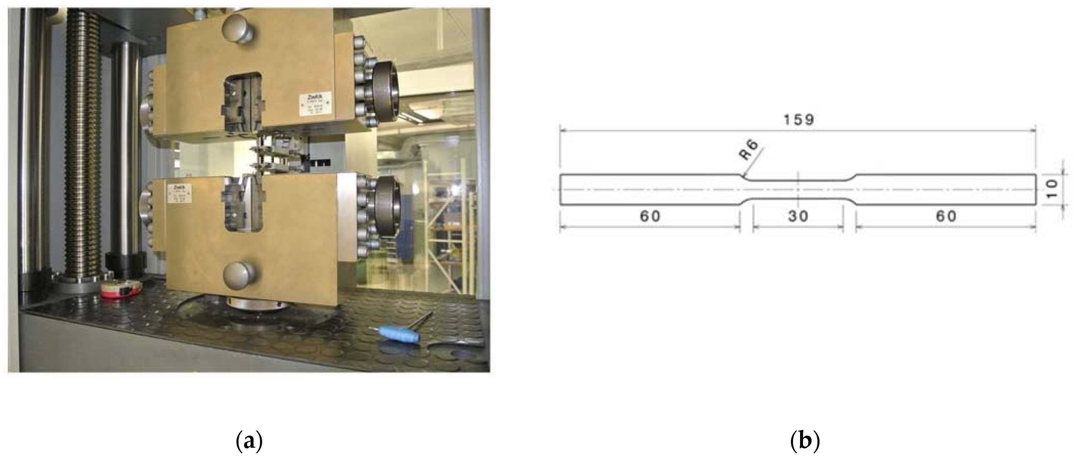
Contrary to the referenced literature, the dynamic experiment used in the study was designed replicating conditions in which real products operate. Actually, the experiment and the material (structural steel E185, formerly Fe310-0 according to standard ISO 630:1995 A1:2003) were used in a pilot project of the plastic turbocharger frame design. In this project, sheets of this material were intended to be used as a shield to contain moving particles inside the frame in case of a turbocharger burst. Due to its abilities in terms of plastic deformation and the low cost-efficiency, this material was adequate for our application.
There are many known evolutionary algorithms to solve multi-dimensional optimisation problems, e.g., particle swarm optimisation (PSO) [27], diferential evolution (DE) [28], biogeography-based optimisation (BBO) [29] social network optimisation (SNO) [30]. The applied evolutionary optimisation algorithm in this research was mainly selected based on our previous experiences. For different past studies [31] in our research group, a few evolutionary algorithms were analysed, in particular PSO, some versions of genetic algorithms [32,33], and differential ant stigmergy algorithm (DASA) [34]. It is known that optimisation results can be quite affected by the algorithm’s parameter settings and in our past studies the most consistent behaviour with the same parameter settings for different applications showed the real valued genetic algorithm (RVGA) [33] and the DASA [34]. The problem with the PSO was that different settings had to be set practically for each study to get optimum results, while the settings for the DASA or the RVGA were tuned through the first few studies and since then these parameter settings have not been changed and they have given us the optimum results in different researches.
The key contributions of this study are:
  • The main objective is to obtain the optimum values for characterising the material behaviour of the structural steel E185 at low, medium and high strain rates, which are difficult to find in the literature. In most cases they can only be found for high-strain-rate applications.
  • It is shown that the optimum material parameters can be estimated on the basis of non-standardised experimental results using a reverse-engineering approach.
  • A first comparison among the modelled response surfaces based on different DoE techniques and different modelling settings is performed and presented.
  • The second comparison among three optimisation algorithms, i.e., the traditional gradient descent (GD), the real-valued genetic algorithm (RVGA) and the differential ant-stigmergy algorithm (DASA), is presented to evaluate their effectiveness on the given response surfaces.
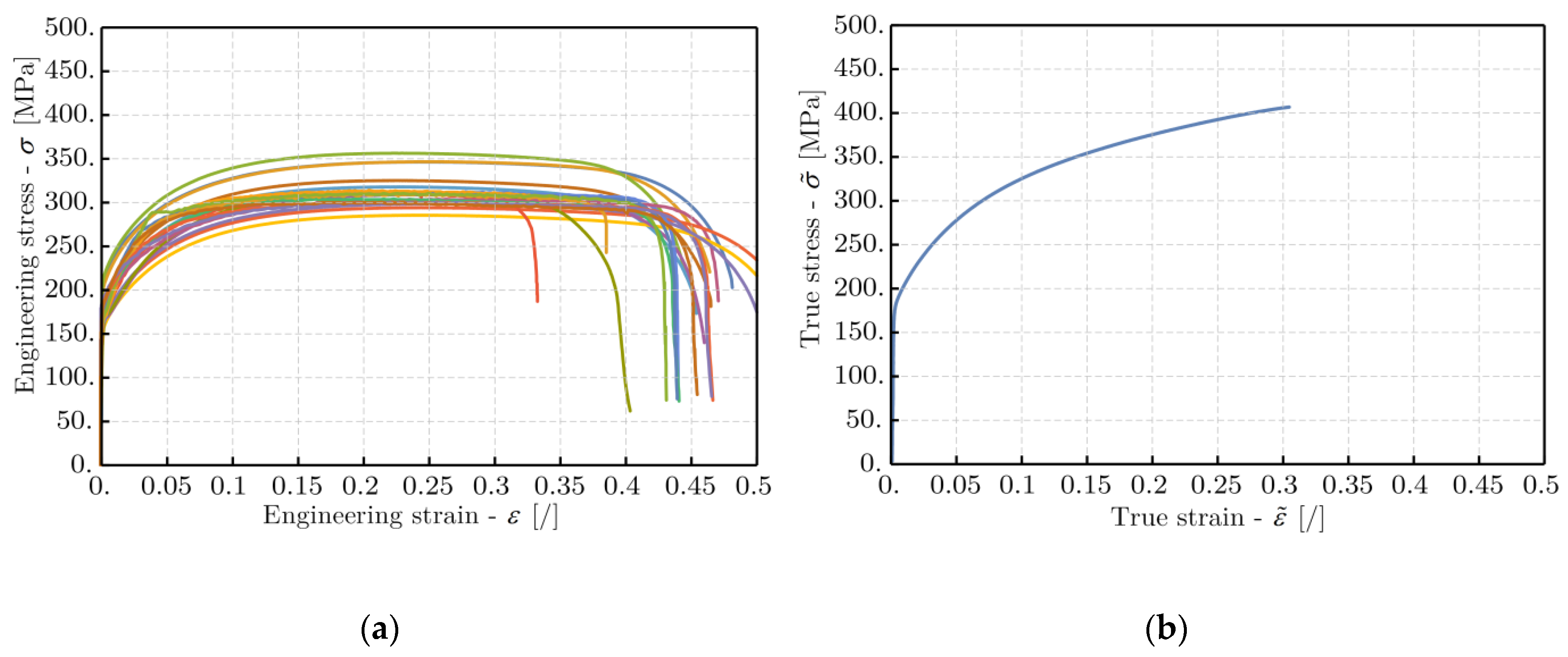
The article consists of five sections, and is structured as follows. After the introduction, an experimental setup within low and medium strain rates, static curve results and dynamic test results are presented. The article continues with 
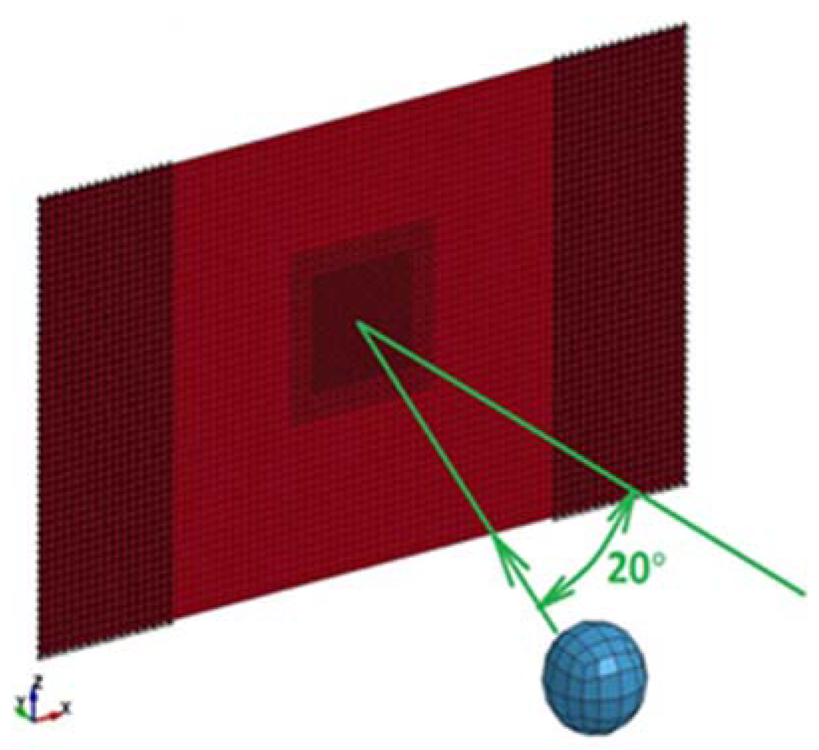
Section 3, where the applied methodology is briefly presented. First, the explicit finite-element model and the required parameters for the J-C material model are described. Then, a cost function is given, which includes the results from both experiments and simulations, and a selection approach using the Taguchi orthogonal array to model the response surface is shown. In Section 4, the results are presented and discussed, together with comparisons with other optimisation methods and values from the literature. Finally, the conclusions and suggestions for future work are given.

2. Experimental Arrangement

The experimental arrangements for the static and dynamic conditions were carried out to obtain the results that formed the basis of our approach. The static material properties (modulus of elasticity, yield stress, ultimate tensile stress) were measured on a Zwick/Roell Z050 test rig according to the ASTM E8/E8M standard [35]. To study the dynamic behaviour, a similar experimental setup to that described in the ASTM D5420 standard [36] was designed, i.e., a standard on a test method to measure the impact resistance of a flat plastic specimen subjected to a drop weight.

2.1. Measuring a Static Stress-Strain Curve

The specimen geometry together with the Zwick/Roell test stand is shown in Figure 1. To obtain the reference stress-strain curve of the observed material, 21 tensile tests with a controlled loading speed of 100 mm/min were performed. The average yield stress and the ultimate tensile stress from the tensile tests were about 185 MPa and 350 MPa, respectively. The resulting true-stress vs. true-strain curve from the measured engineering stress-strain curves is presented in Figure 2. This true-stress vs. true-strain curve was calculated according to Equations (1) and (2) and fitted to all the measured curves using the least-squares method. The chemical composition of the observed material is listed in Table 1.
ε ˜ = ln ( 1 + ε )
σ ˜ = σ ( 1 + ε )
ε and σ were the corresponding average engineering strain and stress, respectively.
The material properties acquired from the presented tests (Young’s modulus, Poisson’s ratio and yield stress) were used in the J-C material model, while the average true-stress vs. true-strain curve was used as the quasi-static reference conditions ( ε ˙ 0 = 0.056 s−1). With the correct parameter values for the J-C material model, a curve calculated with Equation (3) should be fitted to the reference quasi-static curve.

2.2. Experimental Determination of the Material Behaviour at Higher Strain Rates

In our experimental setup, a steel ball with a diameter of 14 mm and a weight of 11 g was shot at a flat specimen at an angle of 20° with different velocities depending on the specimen thickness. Due to the limitations of the air gun used as part of the experimental setup, the lowest striking velocity was 100 m/s and the maximum velocity was chosen so that the impact of the ball did not cause cracks in the specimen, which happened at about 165 m/s. The specimens were sheet-metal plates measuring 98 mm × 60 mm and two different thicknesses (1 mm and 1.5 mm).
The specimens were fixed along the shorter side of the sample; therefore, the free area of the specimen was 60 × 60 mm2. At least three impact tests were performed for each written combination of sheet thickness and impact velocity (except for one combination of sheet thickness and impact velocity). The average experimental results for 16 measurements, together with the standard deviation for the indentation depth and the position of the indentation centre (Figure 3), are presented in Table 2.
The results in Table 2 show that the scatter of the experimental results is relatively small, which means that the experimental design was appropriate for the study. Furthermore, it is clear that the indentation depth increases with an increasing velocity. With a thickness of 1.5 mm, the indentation depth is smaller than with the 1-millimetre-thick steel plate. Another clearly observed feature of the different thicknesses is the point with the deepest indentation depth. For the samples with a thickness of 1.5 mm, this point lies approximately in the centre of the impact. On the 1-mm-thick samples, however, the point with the largest indentation depth is about 5 mm from the centre of the impact (Table 2). This implies different impact dynamics for the specimens of different thicknesses, and this should be replicated by the numerical simulations if the strain-rate parameters of the J-C material model are properly identified.

3. Identification of the Optimum Parameter Values for the Johnson-Cook Material Model

3.1. FE Model for the Identification of the Material Parameters

To identify the material parameters of the J-C material model [4,8,37], the LS-DYNA explicit, dynamic, finite-element code was used, whereby the investigated material model is implemented in its original and simplified forms. The original J-C model considers temperature effects, but in our case, these were neglected, and the parameter m was set to 0.
σ flow = [ σ 0 + B ( ε eff p ) n ] [ 1 + C ln ( ε ˙ p ε ˙ 0 ) ] ( T T room T melt T room ) m ,
Therefore, the simplified J-C (MAT98) material model from the LS-Dyna package software [37] (p. 1697) was applied. It is defined by the following parameters: material density, modulus of elasticity, Poisson’s ratio, yield stress σ 0 , and the three parameters B, n and C, which describe the plastic flow stress and the strain-rate effect. The values of the first four parameters were determined from the static tensile test shown in Section 2.1: the material density was 7850 kg/m3, the modulus of elasticity 2.1·105 N/mm2, the yield stress σ 0 = 180 MPa at a reference strain rate ε ˙ 0 = 0.056 s−1 (see Figure 2) and the Poisson’s ratio ν = 0.3. The last three parameters (B, n, C) cannot be easily estimated from a tensile test like the elastic modulus or the yield stress and are determined differently. One possibility is to perform the tensile or compressive tests at different loading rates and estimate the parameter values using statistical methods [13,14,18], but tensile-test rigs usually have loading-rate limits that prevent very high strain rates. The other possibility is to apply a reverse-engineering approach using numerical simulations that reproduce the actual experiment [15,16,17,26,27], where the loading-speed conditions could have the same values as in real applications where exact strain rates cannot to be estimated. The latter approach is also more convenient when the stress-strain results from tensile or compressive tests at higher loading speeds are not available, as in our case.
The finite-element model used to simulate the ball-impact experiment from Section 2.2 is shown in Figure 4. The steel-sheet model has 5436 four- and three-node-shell finite elements. The mesh density around the impact area is greater than in the wider region of the specimen model in order to accurately simulate the indentation. The rigid ball is modelled with 448 solid finite elements. In the finite-element model, there are fixed nodes for all the degrees of freedom on both sides of the thin plate (Figure 4).
A rigid ball is shot into the centre of the plate at an angle of 20° with different velocities, which are listed in Table 2. There is an automatic surface-to-surface contact between the steel plate and the rigid ball with a coefficient of friction μ = 0.2. The strain on the left-hand side of the plate and the gross geometric dimensions of the specimen were recorded during the simulation for further processing, as in the experiment (Figure 3). For the investigated material model, the strain rate influences the flow stress σ f l o w across its entire range and its non-linearity depends on the exponent n. The higher the strain rate, the higher the flow-stress curve. This means that under quasi-static conditions ( ε ˙ 0 = 0.056 s−1) the true-stress vs. true-strain curve, calculated from [37] (p. 1697) with the correctly determined parameters B, n and C, should be very similar or the same as the experimental curve from the static tensile test.
In order to estimate the optimum values of the observed material parameters for a wide range of strain rates (from quasi-static to high strain rates) the optimisation process must be carried out in such a way that the results from the static and the dynamic experiments can be included. This is the main reason why the two experimental arrangement results from Section 2 (the data from the impact test and the static true-stress vs. true-strain curve) are essential for the proposed procedure.

3.2. Determination of the Cost Function

In order to identify the optimum combination of the applied material model parameters, we carried out a procedure in which we combined an explicit, dynamic finite-element method, a method for DoEs, the modelling of a response surface and an optimisation algorithm.
To estimate the parameter values of the J-C material model (B, n, C) a series of numerical simulations should be performed with different combinations of material parameters to obtain the combination that best fits the experimental results. The main problem is the range of possible parameter values, which can span many orders of magnitude, so that numerous parameter combinations and thus numerical simulations can occur. To reduce the number of numerical simulations, modelling the response surface in a design space of parameters can be particularly useful. In this way, the response surface can be used to search for the optimum combination of parameters. First, a cost function should be properly determined and its values together with combinations of parameter values represent the exact points of the response surface.
For this reason, we designed a four-dimensional design space, where three independent parameters of the J-C material model (i.e., B, n, C) represent the search domain, and the cost function is a dependent variable. To find the optimum material parameter values for the observed material model, it is necessary to define a cost function in which the experimental results for the quasi-static and dynamic conditions from Section 2 can be used. Thus, the optimum combination of parameter values might be suitable for high and intermediate strain rates (for which the J-C model was primarily intended) and also for low strain rates (to obtain the same stress-strain curve under quasi-static conditions). Consequently, the cost function for the optimisation procedure was a weighted sum of the squared differences between the experimentally determined and simulated dynamic load data and a weighted sum of the area differences between the experimentally determined and the calculated static curves:
f ( B , n , C ) = w stat f ( B , n , C ) stat + w dyn f ( B , n , C ) dyn .
For a dynamic load, two post-impact geometrical deformation parameters of the specimen were inspected: the indentation depth and the position of the indentation centre. The cost function is defined as follows:
f ( B , n , C ) dyn = 1 n ( w i = 1 n ( H exp H sim ) 2 + ( 1 w ) i = 1 n ( Z exp Z sim ) 2 )
where n is the number of experimental results with different boundary conditions and w is the weighting factor. Hexp, Zexp, Hsim, and Zsim are the indentation depth and its z-coordinate of the specimen for the average measurements and simulations, respectively. In our case, n and w were equal to 6 and 0.5, respectively.
The trapezoidal integration rule was used to calculate the area differences between the experimentally determined and the calculated curve:
f ( B , n , C ) stat = i = 1 n 1 Δ x ( | Y calc , i Y exp , i | + | Y calc , ( i + 1 ) Y exp , ( i + 1 ) | ) 2 ,
where n is the number of points for each stress-strain curve (experimental and calculated), Yexp is the y component of the experimental stress-strain curve’s points and Ycalc is the y component of the calculated stress-strain curve’s points. In addition, the results for the static case had to be divided by a factor of 10 to achieve a similar size range compared to the dynamic case.
The combinations of the input parameter values and the corresponding cost-functions were defined as points in a four-dimensional design space. Using these points, we created a response surface using the global-local modelling method. Consequently, we obtained a mathematical function that passed through each point in the observed design space defined by the parameter values and the corresponding cost function. The global trend of the response surface f(x1, x2, x3) was modelled with a full multivariate polynomial of the third degree [26], Equations (3) and (7). The local deviations of the cost functions from the global trend ri were modelled with a mixture of multivariate elliptical Gaussian functions [26], Equations (3) and (9) with diagonal covariance matrices (see [26] for details). The diagonal elements of the individual covariance matrices were calculated on the basis of the distance to the nearest neighbour along the corresponding coordinate axis. Before calculating the variance, the nearest-neighbour distance was modified with a scaling factor. Two scaling factors were studied in this research, i.e., the scaling factors of 0.40 and 0.45. Values smaller than that are inappropriate, because they result in poor smoothing of the local response-surface geometry. Larger values cause an over-smoothing effect, which is not good for our purpose. This mathematical function was subsequently used in the optimisation process to identify the optimum parameter values.
f ( x 1 , x 2 , x 3 ) = a 0 + r = 1 3 i = 1 3 a r , i x i r + a 2 , 4 x 1 x 2 + a 2 , 5 x 1 x 3 + a 2 , 6 x 2 x 3 + a 3 , 4 x 1 2 x 2 + a 3 , 5 x 1 x 2 2 + + a 3 , 6 x 1 2 x 3 + a 3 , 7 x 1 x 3 2 + a 3 , 8 x 2 2 x 3 + a 3 , 9 x 2 x 3 2 + a 3 , 10 x 1 x 2 x 3
r i = j = 1 n b j w j ( x i x j , Σ j ) = j = 1 n b j 1 ( 2 π ) 3 | Σ j | e ( 1 2 ( x i x j ) T Σ j 1 ( x i x j ) ) , i = 1 , , n

3.3. Selection of the DoE Technicque

The approximation accuracy of the modelled response surface depends on the number of determined parameter combinations and the dimensions of the design space. Each parameter has its own number of levels and since the range of each parameter spans more than one order of magnitude, the logarithms of these values were used. To have a very accurate response surface, as many parameter combinations as possible should be considered, but this leads to a problem in terms of processing time. When a large number of simulations needs to be carried out, and if the simulation’s calculation time, as in our case, is about two hours, this can be a very time-consuming process, even if the simulation calculations are run in parallel. Therefore, a suitable number of simulations should be chosen, depending on the parameter levels.
For example, if a full-factorial experiment (FFE) with an appropriate number of parameter levels is used to select these points, it could represent the search space relatively accurately. However, as the level of each parameter increases, the space points multiply exponentially. According to the FFE [1], 125 combination points for five-level parameters in the three-dimensional search space would be required. With six different boundary conditions (for different thicknesses and velocities), this would result in 750 simulation calculations in our case. If only one additional level was used for each parameter, 1296 simulations would result. For this reason, a method to reduce the number of parameter combinations is needed, but at the same time the information in the design space should not be reduced significantly. With a suitable DoE method, the combination points can be distributed approximately equally across the entire search-space domain, with the same parameter levels as in the FFE, but with a lower density of combination points in the search-space domain.
As before [38], we decided to use Taguchi orthogonal arrays (TAs). We applied the L81(340) orthogonal array and transformed it into the L81(910) orthogonal array using a linear graph [24,25]. This was done because many levels per parameter were needed, and the L81(910) was best suited for this requirement. Using the L81(910) orthogonal array, the three material parameters (B, n and C for the J-C material model) are assigned to the first three columns of the L81(910) array. The levels were selected from a narrowed area from the previous study [38], where we found a domain with the best solutions for the J-C material model. In that research, we used an assumed reference static strain rate ( ε ˙ 0 = 1 s−1), which was corrected for this study ( ε ˙ 0 = 0.056 s−1). The same procedure was applied in this article to define the parameter combination points used to model the response surface. For each parameter we used the nearest equidistant logarithmic values in the TA (see Table 3).
In this way, 81 parameter combinations were defined for nine levels of each parameter to cover the entire search domain on which the modelled response surface would be built. Consequently, 486 simulations need to be performed with six different boundary conditions to obtain the values of the cost function, which are almost ten times lower compared to the FFE for the same nine-level parameters.
In addition, a second modelling procedure was carried out using the FFE in the similar search domain with wider ranges of the parameters B and C instead of the orthogonal TA domain (Table 4). This was to verify the accuracy of the response surface modelled using the points defined by TA with the surface modelled using the points defined by the FFE. Since we can define the search-space domain for the modelling of the response surface relatively accurately (depending on the number of parameter levels) in the FFE, we compared it with the TA to find out whether the whole identification process could be shortened without too much impact on the results. The search space boundaries of parameters B and C in the FFE were selected wider from the TA to ensure the optimum point of the response surface was located inside the domain and not at its boundaries and that no better optimum points were missed with the TA procedure.

3.4. Applied Optimisation Algorithms

In the final part of the identification approach we applied a variation of the real-valued genetic algorithm (RVGA) [32,33] as a reference optimisation scheme. Besides that, we also applied two other optimisation methods (traditional and metaheuristic) to compare their performance on the modelled response surface. The traditional one was a gradient-descent method (GD) and the evolutionary one was a differential ant-stigmergy algorithm (DASA) [34]. To obtain properly comparable results, we had to set the same general parameters for the applied algorithms. The evolutionary algorithms had a population of 20 (genomes or ants, depending on the algorithm). Therefore, the GD had 20 randomly selected starting points on a given response surface within the parameter’s limits. The maximum number of iterations or generations was set to 10,000 in order to stop the algorithm. Each algorithm was then repeated 30 times, which was similar in the literature [39], where also comparisons between different algorithm’s performances were carried out. Other settings for the applied algorithms were equal as in the previous studies [31] and are listed in Table 5.

4. Results and Discussion

The finite-element simulations of the experimental setup were performed on a numerical server with two Intel Xeon X5670 processors operating at 2.93 GHz, with 48 GB of RAM and a Linux operating system. The average time required for a numerical simulation on a processor core was about one hour and the maximum calculation time was set to two hours. The time limit was triggered if the calculation time step during the simulation was reduced below reasonable values and the simulation termination time could not be reached. To also be able to include in the optimisation process the results from the calculations with error termination, we set their values to the maximum.

4.1. Comparison of the Results Based on the DoE Techniques

Table 6 and Table 7 show five minimum cost-function values from the modelled surface and the optimum solved by the RVGA, GD and DASA together with their parameter combinations. It turned out that more consistent optimisation results were obtained if the nearest-neighbour distance was scaled with a factor of 0.45 to obtain diagonal covariance matrices for the local modelling of the cost function. All the results in the continuation are, therefore, presented using this scaling factor. Both DoE approaches gave similar results, especially for the values of the parameters B and n, although in the TA the DoE had 10 times fewer combinations for modelling the response surface. The values of the parameters n and C from the response-surface points are different for the two DoE approaches, but of the same order of magnitude. We can see that, in the FFE DoE approach, only the values of the parameter C vary between five points with minimum values of the cost function, while in the TA DoE approach, the value of the parameter B also varies between these points.
The following figures (Figure 5 and Figure 6) show the points of the calculated cost function from the Taguchi array (TA) and the full-factorial experiment (FFE) with the corresponding response surfaces in the four-dimensional design space. The parameter’s logarithmic values from Table 3 and Table 4 are the coordinates of a single combination point and its colour represents the corresponding logarithmic value of the cost function. In the two figures on the right we see two modelled response surfaces (the FFE and TA modelled response surface), which have similar shapes for the two cases. Although the FFE modelled response surface has wider ranges of the parameters B and C (see Table 4), it is limited to the similar domain as the TA modelled response surface in the Figure 6. This is only to clearly present similarities between both modelled surfaces with quite different set of modelling points in the observed search space.
The domain of points with minimum values of the cost function (purple region) extends almost vertically through the design space as a kind of 3D curve surrounded by areas of points with higher values (the blue and green regions). A red region (the points with the highest values of the cost function) is located on the outside (FFE modelled) or at the edges of the design space under consideration (TA modelled). The optimum combination of the FFE-modelled response surface (a single grey point on the left-hand-side graphs) is located around very similar values in both response surfaces, although the value of the parameter n is slightly different. On the TA-modelled response surface, the purple region is wider and extends almost to the highest limit of the parameter n. The main reason for this extension is the lack of points in its vicinity defined by the Taguchi array. By selecting the Taguchi array differently, we would be able to define more points in this zone and obtain a more accurate response surface. Regardless of this, we obtained very similar optimum parameter values with the Taguchi array, although we had very few defined points around the actual optimum.

4.2. Comparison of the Results from the Optimisation Algorithms

Table 8 and Table 9 show the results for a comparison of all three optimisation algorithms. For each algorithm the average values and the standard deviations of the final cost function from the 30 repeated runs are presented. For each repetition, the initial values of the parameters were set randomly from different search-space points. Given these results, we can see that all the methods received similar parameter values for the J-C material model, although there were some differences. Furthermore, there were also time calculations to evaluate which algorithm would perform best.
For the TA-modelled response surface (Table 8), the best average value of the cost functions was achieved using the GD and the standard deviations of the best values obtained in each repetition were relatively small, indicating a very small dispersion of the resulting cost-function values. Thus, the most consistent results were given by the GD, which also achieved the minimum cost function in this procedure (Table 6). The other two algorithms achieved practically the same average values, which were about 10% higher than in the GD, but the scatter of the resulting cost-function values was higher. This shows the standard deviation, which is approximately twice as high in the RVGA as in the DASA and ten times higher than in the GD.
This was not the case in the FFE-modelled response surface (Table 9), where the best average value of the cost function was obtained from the DASA with the smallest scatter of the best cost-function values. The RVGA had 6% higher average values, but with a much greater dispersion, showing that the DASA was able to provide us with more consistent results in the FFE. The performance of the GD was much worse in this case, as the average value obtained was three times higher than the average value obtained with the DASA and also the standard deviation of the cost-function values was more than ten times higher. The reason for this is the much larger search space in the FFE process, and it happened that the GD was trapped in a local optimum, from which it could not escape. If the search space had been narrowed, like with the TA-modelled surface, the GD would probably also have been more competitive with the FFE surface.
In terms of calculation time, the best performance was obtained with the RVGA; the DASA was 10% slower and the GD was three to ten times slower compared to the other two. Even though the RVGA was 10% faster than the DASA, both algorithms achieved practically the same results, especially regarding the minimum values of the cost function. In conclusion, all three algorithms showed similar results, thus, all of them could be competitive for our presented procedure. If we take into account the well-known disadvantages of the GD method (which sometimes cannot escape from a local minimum) and the calculation time, the best performance in our procedure was achieved with the DASA algorithm.

4.3. Comparison of the Results with the Data in the Literature

In the final comparison we used the parameter values from Table 6 and Table 7 for each algorithm in both modelled response surfaces. With these parameter values we simulated the dynamic experiment from Section 2.2 to obtain the real cost-function values for the modelled optimum parameter values. These results gave us the final information about the accuracy of the modelled response surface. We can see (Table 10) that with the TA procedure the most accurate cost-function value was obtained with the GD, while with the FFE procedure the most accurate was defined by the other two algorithms. Although the cost-function values calculated from the simulations are different, we have to take into account how much information about the cost function was known in the vicinity of the optimum values.
In the last table (Table 11) we compared the obtained parameters in our TA procedure with some from the literature. It is clear that our values are comparable to those in literature, although those were achieved with a completely different dynamic experiment (mostly the SHB test or the Taylor test). Furthermore, with a correctly defined reference strain rate under quasi-static conditions, the values of the parameter C are also similar or the range of those in the literature data.

5. Conclusions

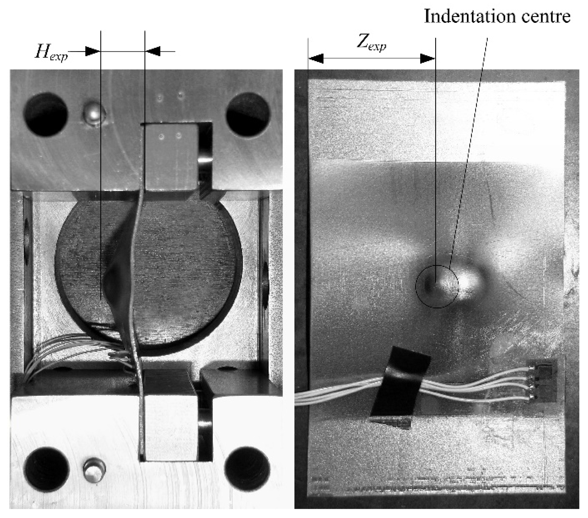
This article presents a general approach to estimate the parameters that determine the behaviour of a material subjected to high strain rates. In our approach, the Taguchi experimental design was combined with the finite-element code LS-DYNA, the modelled response surface and three optimisation algorithms to estimate the material parameters based on the results of a standard static tensile test and a non-standard impact test between a ball and a thin sheet. With a reverse-engineering procedure and a completely different experiment, when compared to the literature data, the presented approach was applied to the realistic case of a material parameter estimation for the Johnson-Cook material model at low and intermediate values of the strain rates. Additionally, the second approach was performed using a full-factorial DoE technique to compare the accuracy of the presented approach.
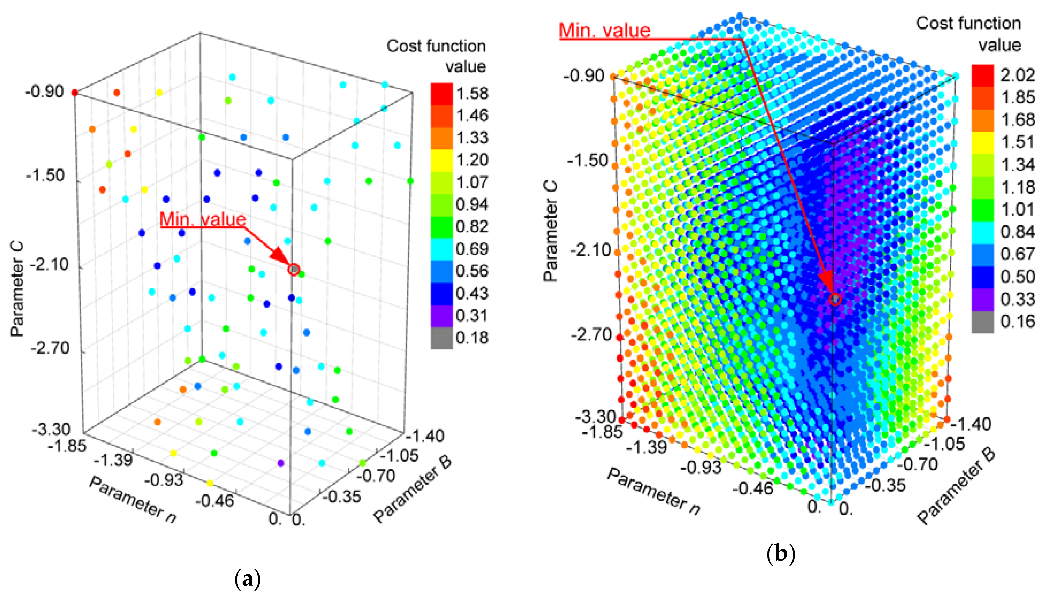
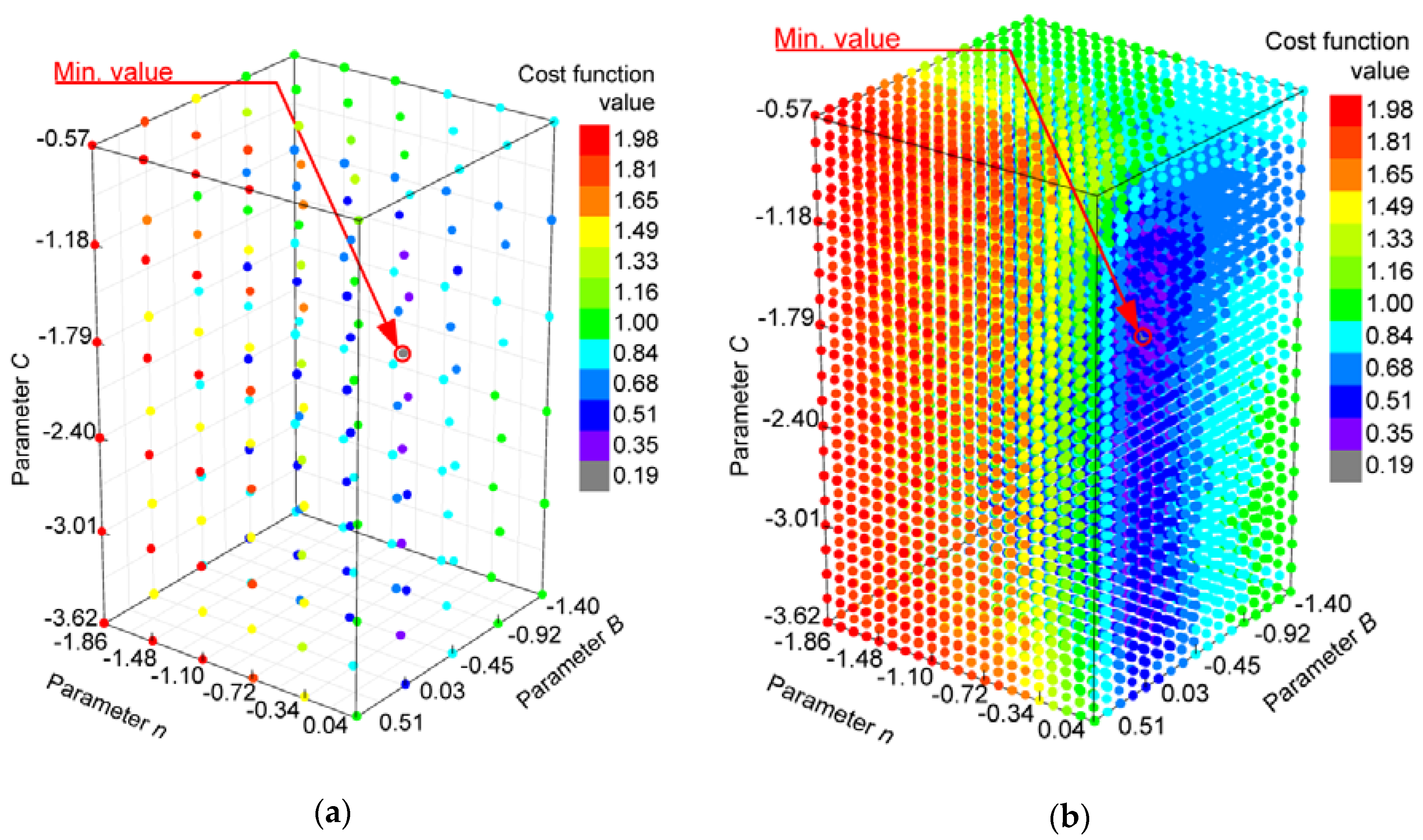
It turned out that it is possible to obtain reliable estimates of the Johnson-Cook parameters (B, n, C) with a suitable design-of-simulation approach using only two iteration runs, i.e., first with the wide-domain approach from which the narrower domain of the design space was isolated. Nevertheless, even with two iteration runs using the Taguchi-array approach, the total number of simulations was significantly lower than with the full-factorial arrangement of the design-space combinations in the narrower domain. The optimisation process based on TA points had 2.5 times less simulations for the similar range of parameters, but with higher number of parameter levels as the optimisation process based on the FFE points. If the calculation time for the whole TA procedure is accounted, this is approximately more than two times faster than for the FFE procedure. Further, it was shown that the GD algorithm found a better optimum with a smaller dispersion in 30 repetitions on the TA modelled response surface as the other two algorithms, even though it was much slower. On the FFE modelled response surface the two metaheuristic algorithms were evidently better. The most consistent results were given by DASA, but with slightly slower calculation time than RVGA. Moreover, the estimated material parameters for the observed material model are consistent and comparable with the results from the literature. The results from our study are practically in the same order of magnitude. The optimum value of parameter B is about 30% higher in comparison with [17,21] but two times smaller than [18], while the optimum value of the parameter n is in the middle of the range found in the literature and the optimum value of the parameter C is in fact the lowest in comparison with those from the literature, but only 10% lower than the smallest value reported in [17].

Author Contributions

All authors contributed equally in this research paper. All authors have read and agreed to the published version of the manuscript.

Funding

This research was funded by the Slovenian Research Agency (ARRS), grant research programme P2-0182 (R&D evaluations—Razvojna vrednotenja).

Conflicts of Interest

The authors declare no conflict of interest

Nomenclature and Abbreviations

nJohnson-Cook material parameterRVGAreal valued genetic algorithm
tspecimen thicknessTATaguchi array
vball velocityZexpz-coord. of ind. centre from experiment
wcost function weightZsimz-coord. of ind. centre from simulation
BJohnson-Cook material parameter ε engineering strain
CJohnson-Cook material parameter ε ˜ true strain
DASAdifferential ant stigmergy algorithm ε ˙ strain rate
DoEdesign of experiment ν Poisson’s number
FFEfull factorial experiment μ coefficient of friction
GDgradient descent σ engineering stress
Hexpheight of indentation from experiment σ ˜ true stress
Hsimheight of indentation from simulation σ flow plastic flow stress
J-CJohnson-Cook σ 0 yield stress

References

  1. Ryan, T.P. Modern Experimental Design, 3rd ed.; John Wiley & Sons Inc.: Hoboken, NJ, USA, 2007; 624p. [Google Scholar]
  2. Wagner, J.R.; Mount, E.M.; Giles, F.H. 25-Design of experiments. In Extrusion, 2nd ed.; Wagner, J.R., Mount, E.M., Giles, F.H., Eds.; William Andrew Publishing: Oxford, UK, 2014; pp. 291–308. [Google Scholar] [CrossRef]
  3. Giunta, A.; Wojtkiewicz, S.; Eldred, M. Overview of modern design of experiments methods for computational simulations. AIAA 2003, 0649. [Google Scholar] [CrossRef]
  4. Johnson, G.R.; Cook, W.H. A constitutive model and data for metals subjected to large strains, high strain rates and high temperatures. In Proceedings of the 7th International Symposium on Ballistics, The Hague, The Netherlands, 19–21 April 1983. [Google Scholar]
  5. Zerilli, F.J.; Armstrong, R.W. Dislocation-mechanics-based constitutive relations for material dynamics calculations. J. Appl. Phys. 1987, 61, 1816–1825. [Google Scholar] [CrossRef] [Green Version]
  6. Armstrong, R.W.; Walley, S.M. High strain rate properties of metals and alloys. Int. Mater. Rev. 2008, 53, 105–128. [Google Scholar] [CrossRef]
  7. El-Magd, E. Mechanical properties at high strain rates. J. Phys. IV Fr. 1994, 4, 149–170. [Google Scholar] [CrossRef]
  8. Hallquist, J.O. LS-DYNA Theoretical Manual; Livermore Software Technology Corporation: Livermore, CA, USA, 1998. [Google Scholar]
  9. Paul, S.K.; Raj, A.; Biswas, P.; Manikandan, G.; Verma, R.K. Tensile flow behavior of ultra low carbon, low carbon and micro alloyed steel sheets for auto application under low to intermediate strain rate. Mater. Des. 2014, 57, 211–217. [Google Scholar] [CrossRef]
  10. Yu, H.; Guo, Y.; Zhang, K.; Lai, X. Constitutive model on the description of plastic behavior of DP600 steel at strain rate from 10−4 to 103 s−1. Comput. Mater. Sci. 2009, 46, 36–41. [Google Scholar] [CrossRef]
  11. Paul, S.K. Predicting the flow behavior of metals under different strain rate and temperature through phenomenological modeling. Comput. Mater. Sci. 2012, 65, 91–99. [Google Scholar] [CrossRef]
  12. Song, R.; Dai, Q. Dynamic deformation behavior of dual phase ferritic-martensitic steel at strain rates from 10−4 to 2000 s−1. J. Iron Steel Res. Int. 2013, 20, 48–53. [Google Scholar] [CrossRef]
  13. Iqbal, M.A.; Senthil, K.; Bhargava, P.; Gupta, N.K. The characterization and ballistic evaluation of mild steel. Int. J. Impact Eng. 2015, 78, 98–113. [Google Scholar] [CrossRef]
  14. Verleysen, P.; Peirs, J.; Van Slycken, J.; Faes, K.; Duchene, L. Effect of strain rate on the forming behaviour of sheet metals. J. Mater. Process. Technol. 2011, 211, 1457–1464. [Google Scholar] [CrossRef]
  15. Grazka, M.; Janiszewski, J. Identification of Johnson-Cook Equation constants using finite element method. Eng. Trans. 2014, 60, 215–223. [Google Scholar]
  16. Kurtaran, H.; Buyuk, M.; Eskandarian, A. Ballistic impact simulation of GT model vehicle door using finite element method. Theor. Appl. Fract. Mech. 2003, 40, 113–121. [Google Scholar] [CrossRef]
  17. Marais, S.T.; Tait, R.B.; Cloete, T.J.; Nurick, G.N. Material testing at high strain rate using the split Hopkinson pressure bar. Lat. Am. J. Solids Struct. 2004, 1, 319–337. [Google Scholar]
  18. Singh, N.K.; Cadoni, E.; Singha, M.K.; Gupta, N.K. Dynamic tensile and compressive behaviors of mild steel at wide range of strain rates. J. Eng. Mech. 2013, 139, 1197–1206. [Google Scholar] [CrossRef]
  19. Soliman, M.S.; El Rayes, M.M.; Abbas, A.T.; Pimenov, D.Y.; Erdakov, I.N.; Junaedi, H. Effect of tensile strain rate on high-temperature deformation and fracture of rolled Al-15 vol% B4C composite. Mater. Sci. Eng. A 2019, 749, 129–136. [Google Scholar] [CrossRef]
  20. Liang, R.; Khan, A.S. A critical review of experimental results and constitutive models for BCC and FCC metals over a wide range of strain rates and temperatures. Int. J. Plast. 1999, 15, 963–980. [Google Scholar] [CrossRef]
  21. Vedantam, K.; Bajaj, D.; Brar, N.S.; Hill, S. Johnson-Cook strength models for mild and DP 590 steels. AIP Conf. Proc. 2006, 845, 775–778. [Google Scholar] [CrossRef]
  22. Schwer, L. Optional strain-rate forms for the Johnson-Cook constitutive model and the role of the parameter Epsilon_0. In Proceedings of the 6th European LS-DYNA Users’ Conference, Gothenburg, Sweden, 29–30 May 2007. [Google Scholar]
  23. Tanimura, S.; Tsuda, T.; Abe, A.; Hayashi, H.; Jones, N. Comparison of rate-dependent constitutive models with experimental data. Int. J. Impact Eng. 2014, 69, 104–113. [Google Scholar] [CrossRef]
  24. Taguchi, G. System of Experimental Design: Engineering Methods to Optimize Quality and Minimize Costs; American Supplier Institute: Dearborn, MI, USA, 1987; Volume 1. [Google Scholar]
  25. Taguchi, G. System of Experimental Design: Engineering Methods to Optimize Quality and Minimize Costs; American Supplier Institute: Dearborn, MI, USA, 1987; Volume 2. [Google Scholar]
  26. Škrlec, A.; Klemenc, J. Parameter identification for a Cowper-Symonds material model using a genetic algorithm combined with a response surface. Eng. Comput. 2017, 34, 1–29. [Google Scholar] [CrossRef]
  27. Poli, R.; Kennedy, J.; Blackwell, T. Particle swarm optimization. Swarm Intell. 2007, 1, 33–57. [Google Scholar] [CrossRef]
  28. Price, K.V. Differential evolution. In Handbook of Optimization: From Classical to Modern Approach; Zelinka, I., Snášel, V., Abraham, A., Eds.; Springer: Berlin/Heidelberg, Germany, 2013; pp. 187–214. [Google Scholar] [CrossRef]
  29. Simon, D. Biogeography-based optimization. IEEE Trans. Evol. Comput. 2008, 12, 702–713. [Google Scholar] [CrossRef] [Green Version]
  30. Niccolai, A.; Grimaccia, F.; Mussetta, M.; Gandelli, A.; Zich, R. Social network optimization for WSN routing: Analysis on problem codification techniques. Mathematics 2020, 8, 583. [Google Scholar] [CrossRef] [Green Version]
  31. Klemenc, J. Optimization of a modified Locati method using evolutionary algorithms. Exp. Tech. 2016, 40, 947–958. [Google Scholar] [CrossRef]
  32. Temby, L.; Vamplew, P.; Berry, A. Accelerating Real-Valued Genetic Algorithms Using Mutation-with-Momentum. In AI 2005: Advances in Artificial Intelligence; Zhang, S., Jarvis, R., Eds.; Springer: Berlin/Heidelberg, Germany, 2005; Volume 3809, pp. 1108–1111. [Google Scholar] [CrossRef] [Green Version]
  33. Wright, A.H. Genetic algorithms for real parameter optimization. In Foundations of Genetic Algorithms; Rawlins, G.J.E., Ed.; Elsevier: Amsterdam, The Netherlands, 1991; Volume 1, pp. 205–218. [Google Scholar] [CrossRef]
  34. Korošec, P.; Šilc, J.; Filipič, B. The differential ant-stigmergy algorithm. Inf. Sci. 2012, 192, 82–97. [Google Scholar] [CrossRef]
  35. ASTM Standard E8/E8M–09, 2010: Standard Test Methods for Tension Testing of Metallic Materials; ASTM International: West Conshohocken, PA, USA, 2010. [CrossRef]
  36. ASTM Standard D5420-10: Standard Test Method for Impact Resistance of Flat, Rigid Plastic Specimen by Means of a Striker Impacted by a Falling Weight (Gardner Impact); ASTM International: West Conshohocken, PA, USA, 2010. [CrossRef]
  37. Hallquist, J.O. LS-DYNA Keyword User’s Manual-Version 971; Livermore Software Technology Corporation: Livermore, CA, USA, 2007. [Google Scholar]
  38. Škrlec, A.; Klemenc, J. Estimating the strain-rate-dependent parameters of the Cowper-Symonds and Johnson-Cook material models using Taguchi arrays. Stroj. Vestn. J. Mech. Eng. 2016, 62, 220–230. [Google Scholar] [CrossRef] [Green Version]
  39. Jesenik, M.; Mernik, M.; Trlep, M. Determination of a hysteresis model parameters with the use of different evolutionary methods for an innovative hysteresis model. Mathematics 2020, 8, 201. [Google Scholar] [CrossRef] [Green Version]
Figure 1. (a) Zwick/Roell testing device; (b) the sheet specimen for the tensile test.
Mathematics 08 01105 g001
Figure 2. (a) Measured engineering stress-strain curves with a controlled loading speed of 100 mm/min at an ambient temperature 20 °C and for different loading directions in terms of sheet rolling direction (left); (b) True-stress vs. true-strain curve from the average measurement results.
Mathematics 08 01105 g002
Figure 3. Two views of the experimental specimen.
Mathematics 08 01105 g003
Figure 4. 3D model of the experiment.
Mathematics 08 01105 g004
Figure 5. (a) Points defined by Taguchi array (TA); (b) The corresponding response surface (logarithmic values).
Mathematics 08 01105 g005
Figure 6. (a) Points defined by full factorial experiment (FFE); (b) The corresponding response surface (logarithmic values).
Mathematics 08 01105 g006
Table 1. Chemical composition of carbon steel E185 (weight, %).
CMnSiSP
≤0.12≤0.50≤0.30≤0.40≤0.035
Table 2. Combinations of boundary conditions and the results of the experiment.
Experimental Condition NumberSpecimen Thickness
t [mm]
Ball Velocity
v [m/s]
Measured Max. Indentation Depth
Hexp [mm]
Position of the Max. Indentation Depth
Zexp [mm]
AverageSt. deviationAverageSt. deviation
1110311.370.09234.830.648
2110912.120.48134.890.002
3112113.070.07435.110.300
41.512110.380.11630.190.229
5 11.513111.53/29.6/
61.513912.651.60030.490.223
1 For this combination, only one measurement was performed.
Table 3. Parameters levels for the Taguchi array (TA).
Values of Parameter B [GPa]
0.0398110.0595660.0891250.133350.19953
0.298540.446680.668341.000
Values of Parameter n [/]
0.0141250.0240570.0409730.0697830.11885
0.202420.344750.587151.000
Values of Parameter C [/]
0.0005010.0010000.0019950.0039810.007943
0.0158490.0316230.0630960.12589
Table 4. Parameter levels for the full-factorial experiment (FFE).
Values of Parameter B [GPa]
0.040170.12000.35901.0713.200
Values of Parameter n [/]
0.013940.033390.08000.19170.459
1.100
Values of Parameter C [/]
0.0002410.0009820.0040000.016290.0663
0.27011.1004.480018.2400
Table 5. Parameter settings for the RVGA and DASA optimisation algorithms.
Settings for GD Algorithm
Initial step size—h0 0.001
Final error size—e0 0.001
Settings for RVGA
Population size—m20
Probability of crossover—pcr0.5
Fraction of linear crossover—flin0.6
Probability of mutation—pmut0.05
Moment weight—wm1.0
Moment threshold—thm1.0
Settings for DASA
Number of ants—m20
Logarithmic base—10
DASA factor—s+0.02
DASA factor—s0.01
Pheromone evaporation factor—r0.2
Table 6. Taguchi response surface.
Parameter BParameter nParameter CCost Function Value
Point 10.4466870.5871360.0079431.44854
Point 20.4466870.5871360.0112201.47317
Point 30.3651770.5871360.0112201.47763
Point 40.3651770.5871360.0079431.48633
Point 50.3651770.5871360.0158901.50279
RVGA0.3854010.6166930.0171481.43668
DASA0.3854230.6166640.0171481.43668
GD0.4129500.5877330.0089471.42023
Table 7. Full-factorial experiment response surface.
Parameter BParameter nParameter CCost Function Value
Point 10.3584750.4590200.0162851.54070
Point 20.3584750.4590200.0039991.62438
Point 30.3584750.4590200.0080701.64237
Point 40.3584750.4590200.0004871.67314
Point 50.3584750.4590200.0009821.69466
RVGA0.3392250.4496300.0146701.52192
DASA0.3392110.4496300.0146701.52192
GD0.3377600.4466820.0149041.52231
Table 8. Results of the comparison among the applied algorithms for the TA.
RVGADASAGD
Cost-function average values1.56291.56791.4324
Standard deviation2.4925 × 10−19.4369 × 10−21.6443 × 10−2
Calculation time for 30 repetition [s]4045395
Table 9. Results of the comparison among the applied algorithms for the FFE.
RVGADASAGD
Cost-function average values1.66471.56334.4973
Standard deviation3.5692 × 10−13.4237 × 10−29.5355 × 10−1
Calculation time for 30 repetition [s]901001917
Table 10. Comparison of the cost-function values between the modelled and the calculated.
TA—ProcedureFFE—Procedure
Calculated SimulationsResponse SurfaceCalculated SimulationsResponse Surface
RVGA CF—value2.061021.436681.57671.52192
DASA CF—value2.063311.436681.57691.52192
GD CF—value1.875181.420231.66331.52231
Table 11. Comparison with other parameter values in the literature.
Parameter B [GPa]Parameter n [/]Parameter C [/]
Average value from Table 6
(TA—procedure)
0.3950.60.013
Marais et al. [17]0.2920.3100.025
Singh et al. [18]0.779–2.6920.743–0.9280.0144–0.021
Johnson et al. [4], Tanimura et al. [23]0.3800.320.06
Vedantam et al. [21]0.234 0.64280.0756
Paul et al. [9] 1//0.085–0.1
1 In the referenced literature B and n parameters were not reported, only parameter C beside yield stresses in range 0.165−0.190 MPa.

