Abstract
Metaheuristics are smart problem solvers devoted to tackling particularly large optimization problems. During the last 20 years, they have largely been used to solve different problems from the academic as well as from the real-world. However, most of them have originally been designed for operating over real domain variables, being necessary to tailor its internal core, for instance, to be effective in a binary space of solutions. Various works have demonstrated that this internal modification, known as binarization, is not a simple task, since the several existing binarization ways may lead to very different results. This of course forces the user to implement and analyze a large list of binarization schemas for reaching good results. In this paper, we explore two efficient clustering methods, namely KMeans and DBscan to alter a metaheuristic in order to improve it, and thus do not require on the knowledge of an expert user for identifying which binarization strategy works better during the run. Both techniques have widely been applied to solve clustering problems, allowing us to exploit useful information gathered during the search to efficiently control and improve the binarization process. We integrate those techniques to a recent metaheuristic called Crow Search, and we conduct experiments where KMeans and DBscan are contrasted to 32 different binarization methods. The results show that the proposed approaches outperform most of the binarization strategies for a large list of well-known optimization instances.
1. Introduction
Optimization problems can be seen in different areas of the modern world, such as bridge reinforcement [1], load dispatch [2], location of emergency facilities [3], marketing [4], and social networks [5], among others. To solve them, we must identify and understand to which model the problem belongs. There are three types of models, the first has discrete variables, the second has continuous variables, and the third has both types of variables. Discrete optimization has widely been used to define a large number of problems belonging to the NP-hard class [6]. It is necessary to emphasize that the time to solve this type of problem increases exponentially according to its size. For this reason, we consider it totally prudent to solve these problems through metaheuristics [7,8], which deliver acceptable results in a limited period of time.
There are many metaheuristics and we can see a complete collection of all nature-inspired algorithms in [9] but most work on continuous space. Some researchers have been working in depth on developing binary versions that make these metaheuristics operate in binary spaces. A study of putting continuous metaheuristics to work in binary search spaces [10] clearly describes the two-step technique. These techniques require a large number of combinations and tuning of parameters to binarize and thus be able to obtain the best of all, which is a great waste of time.
Despite successful published work, binary techniques require offline analysis and an expert user in the field to adjust the metaheuristic to the problem domain in addition to working with the various available combinations of the two-step technique. Using gained expertise, our work is focused on two binarization clustering methods to smartly modify a set of real solutions to binary solutions by grouping decision variables, without the need for combinations as in the two-step technique, saving time and algorithm manipulation. The first one proposes to use KMeans [11,12] clustering algorithm, the most common unsupervised machine learning algorithm, to assign each variable in defined groups by the user. It is necessary to assign values of transition to each cluster in order to binarize each variable. The second one integrates DBscan [13,14] as a powerful clustering method for arraying values in a nonapriori determined number of clusters. Unlike KMeans, this technique creates the clusters by itself just knowing the number of variables required to be included in a cluster and the distance between each point in the data set. Furthermore, the transition value to binarize is calculated online and depends on each cluster. To test our approaches, we include these clustering methods in the Crow Search Algorithm (CSA) [15] which is a population-based metaheuristic inspired by the behavior of crows (easy implementation, it works very fast, and there are few parameter settings). In this method, each individual follows others trying to discover the places where they hide the food in order to steal it.
Based on [16,17], both works were used as gold standards, and we perform an experimental design led by quantitative methodology. We implement different criteria such as quality of solutions, robustness in terms of the instances, solving large-scale of well known binary optimization problems: Set Covering Problem (SCP) [18] and 0/1 Knapsack Problem (KP) [19]. These two problems are very popular benchmarks to address and try new strategies with because they have known results with which to compare.
The remainder of this manuscript is organized as follows: Section 2 presents the related work. Section 3 exposes binarization strategies. CSA is described in Section 4. Section 5 explains how to integrate binarizations on CSA. Next, experimental results including a research methodology are explained in Section 6. Discussions are shown in Section 7. At the end of the manuscript, conclusions are presented in Section 8.
2. Related Work
As previously mentioned, binarization is mandatory for continuous metaheuristics when the problem ranges in a binary domain. This task is not simple since experimentation with different binarization schemes is needed to reach good results. The transfer function is the most used binarization method and it was introduced in [20]. The transfer function is a very cheap operator, his range provides probabilities values and tries to model the transition of the particle positions. This function is responsible for the first step of the binarization method which corresponds to map the solutions in solutions. Two types of functions have been used in the literature, the S-shaped [21] and V-shaped [22]. The second step is to apply a binarization rule to the result of the transfer function. Examples of binarization rules are a complement, roulette, static probability, and elitist [22]. “Two-step” binarization is employed to refer to the use of transfer functions and binarization rule together. A detailed description of binarization techniques can be seen in [10].
Our goal here is to alleviate the user involvement in binarization testing and to provide a unique alternative that works better on average when contrasted to a large set of “Two-step” binarization techniques. In this context, the use of machine learning techniques appears as a good candidate to support the binarization process and as a consequence to obtain better search processes. Machine learning has already been used to improve search in metaheuristics [23]. For instance, the first trend is to employ machine learning for parameter tuning, as in [24] the authors use machine learning to parameter control in metaheuristics. The techniques reported in this context can be organized in four groups: Parameter control strategies [25], parameter tuning strategies [26], instance-specific parameter tuning strategies [27], and reactive search [28]. The general idea is to exploit search information in order to find good parameter configurations; this may lead to better quality solutions. An example of this is in [29], where the author uses a metaheuristic to determine the optimal number of hidden nodes and their proper initial locations on neural networks. Machine learning has also been used to build approximation models when objective function and constraints are expensive computationally [30]. Population management can also be improved via machine learning algorithms, obtaining information from already visited solutions, and using it to build new ones [31].
Machine learning has also been used to reduce the search space, for instance by using clustering [32] and neural networks [33]. In these works, two main areas of machine learning were used: forecasting and classify. It is important to mention the uses of machine learning with metaheuristics in these areas. It has been used to forecast different kinds of problems, like optimizing the low-carbon flexible job Shop Scheduling problem [34], electric load [35,36] use to forecast economic recessions in Italy, and other industrial problems as in [37]. As we mentioned, machine learning also can be used to classify some different groups of data sets; in this scenario, this technique has also been used in different problems as the image classification [38], electronic noise classification of bacterial foodbones pathogens [39], urban management [40], to mention some recent studies.
Although the participation of machine learning in the metaheuristic field is large, the specific use in binarization is indeed very limited. To the best of our knowledge, only a few experiments with the clustering techniques DBscan and KMeans have been reported [13,41]. In this way, we believe that binarization has a lot of room for exploration beyond the improvement of metaheuristics, the use of just one machine learning technique to binarization, compared to the 32 combinations of two-step technique that let the user gain simplicity, speediness, and less effort to use the binarization on metaheuristics, which is the aim pursued in this work.
3. Binarization
A study of putting continuous metaheuristics to work in binary search spaces [10] exposes two main groups of binarization techniques. The first group called two-step binarization allows one to put in work the continuous metaheuristics without operator modifications and the second group called continuous-binary operator transformation redefines the algebra of the search space, thereby reformulating the operators.
In this work, we used the first group to test our experiments. These two steps refer to transfer functions, which are responsible for mapping solutions in the real domain to a binary domain. Then we are going to use a machine learning strategy of clustering called KMeans in order to cluster the column of solutions and another strategy called DBscan that will cluster all the solutions (matrix). Both strategies will be used to map solutions between 0 and 1.
3.1. Two Step Binarization
Two-step binarization consists of applying, as its name says, two stages in order to bring the variables of the real search space to the world of binary variables. The first step uses eight transfer functions and the second step uses four discretization functions, therefore generating 32 possible strategies to apply.
3.1.1. First Step—Transfer Functions
These operators are very cheap to implement in the algorithm and their range provides probability values and attempts to model the transition of the particle positions; in other words, these functions transform a real solution that belongs to a real domain, to another real solution but restricted to a domain between 0 and 1. For that, there exist two classic types in the literature [42,43] called S-Shape and V-Shape, which are used.
3.1.2. Second Step—Binarization
A set of rules can be applied to transform a solution in the real domain to a solution in the binary domain. We use Standard, Complement, Static probability, and Elitist. In particle swarm optimization, this approach was first used in [20].
3.2. KMeans
KMeans is one of the simplest and most popular unsupervised machine learning algorithms for clustering. The main goal of KMeans [44,45] is to group similar data points given certain similarities. To achieve this objective, a number of clusters in a data set must be set. Then, every data point is allocated to each of the clusters, the arithmetic representation is as follows, see Equation (1):
where k represents the number of clusters, n depicts the number of cases, defines jth case of ith solution, and exposes the lth centroid (see pseudo-code in Algorithm 1).
| Algorithm 1: KMeans pseudo-code |
 |
The mechanism initially requires the k value as the number of the clusters and the best solution vector of dimension d composed by the decision variables . This vector is passed as input data for being grouped (see the left side of Figure 1). Iteratively, KMeans assigns each decision variable to one group based on the similarity of their features and these are allocated to the closest centroid, minimizing Euclidean distances. After, KMeans recalculates centroids by taking the average of all decision variables allocated to the cluster of that centroid, thus decreasing the complete intracluster variance over the past phase.
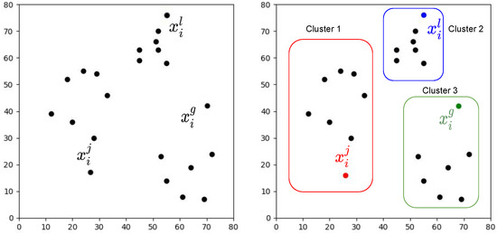
Figure 1.
Clustering process of the KMeans algorithm applied to the decision variables.
The right side of Figure 1 illustrates the computed groups. Positions are adjusted in each iteration of the process until the algorithm converges.
3.3. DBscan
Density-Based Spatial Clustering of Applications with Noise (DBscan) [46] is a well-known data clustering algorithm which is commonly used in data mining and machine learning. It can be used to identify clusters of any shape in a data set containing noise and outliers. Clusters are thick data space areas separated by areas with reduced points density.
The goal is to define thick areas that can be measured by the amount of near-point objects. It is indispensable to know that DBscan has two important parameters that are required for work.
- Epsilon (): Sets how close points should be regarded as part of a cluster to each other.
- Minimum points (MinPts): The minimum number of points to form a dense region.
The main idea is that there must be at least a minimum number of points for each group in the neighborhood of a given radius. The parameter defines the neighborhood radius around a point x, any point x in the data set with a neighbor above or equal to MinPts is marked as a center point, and x is a limit point whether the number of its neighbors is less than MinPts. Finally, if a point is not a core or a point of the edge, then it is called a point of noise or an outer point.
As a summary, this technique helps when you do not know much information about data, see pseudo-code in Algorithm 2.
The right side of Figure 2 illustrates the computed groups. Positions are adjusted in each iteration of the process until the algorithm converges.
| Algorithm 2: DBscan pseudo-code |
 |
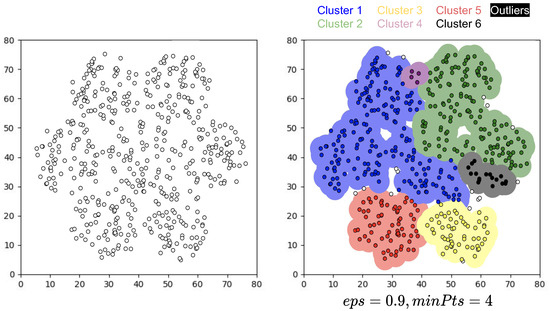
Figure 2.
Clustering process of the DBscan algorithm applied to the best solution.
4. Crow Search Algorithm
Crows (crow family or corvids) are considered the most intelligent birds. They contain the largest brain relative to their body size. Based on a brain-to-body ratio, their brain is slightly lower than a human brain. Evidence of the cleverness of crows is plentiful. They can remember faces and warn each other when an unfriendly one approaches. Moreover, they can use tools, communicate in sophisticated ways, and recall their food hiding place up to several months later.
CSA tries to simulate the intelligent behavior of the crows to find the solution of optimization problems [15]. Optimization point of view: the crows are searchers, the environment is the search space, each position of the crow corresponds to a feasible solution, the quality of food source is the objective function, and the best food source of the environment is the global solution of the problem. Below, parameters for CSA are shown.
- N: Population.
- AP: Awareness probability.
- : Flight length.
- : Maximum number of iterations.
When CSA is working, two things can happen. For this, let Crow 1 and Crow 2 be different possible solutions belonging to the search space. Firstly, Crow 1 does not know that Crow 2 is following it. As a result, Crow 2 will approach the hiding place of Crow 1. This action is called State 1. On the other hand, Crow 1 knows that Crow 2 is following it. Finally, to protect its hidden place from being stolen, Crow 1 will fool Crow 2 by going to another position of the search space. This action is called state 2. The representation of these states is represented for Equation (2).
where:
- and are random numbers with uniform distribution between 0 and 1.
- denotes the flight length of crows.
- denotes the awareness probability of crows (intensification and diversification).
Below, pseudo-code of CSA is shown in Algorithm 3.
| Algorithm 3: CSA pseudo-code |
 |
5. Integration: Binarizations on CSA
As we shown in Section 3, to work in a binary search space CSA [15], one must apply the binarization techniques. Firstly, we will solve the problem using Two-steps technique, then we will apply KMeans technique.
To have a high level explanation, the steps are described below:
When CSA evaluate a , a real value is generated, then:
- Two-steps: in t + 1 is binarized column by column applying the first step getting a continuous solution that enters as an input to the second step making the binarization evaluate the solution in the Objective function.
- KMeans: In this case, in t + 1 is clustered. Then each cluster is assigned to a cluster transition value already defined as a parameter. Small centroids get the small cluster transition value and a high centroid value gets a high value of transition. It is necessary to evaluate every point in the clusters, asking if random values between 0 an 1 are equal or greater than a cluster transition value. If we get the position and apply the complement to the in t, then the objective function is evaluated.
For theses two techniques we take the same strategy that is illustrated in Algorithm 4.
| Algorithm 4: CSA + Two-steps and Kmeans binarization techniques pseudo-code |
 |
A graphic representation can be seen in Figure 3. A continuous solution from the metaheuristic is transformed into a solution that belongs to real domain to a solution in a real domain but restricted to a domain between 0 and 1, applying the first step. Then, the solution again is transformed into a solution in a binary domain using step 2. Figure 4 shows how the real solution is clusterized and then transformed to a binary solution applying cluster transition value using KMeans.
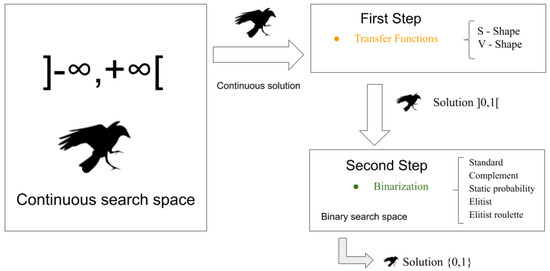
Figure 3.
Continuous to Binary Two-steps.
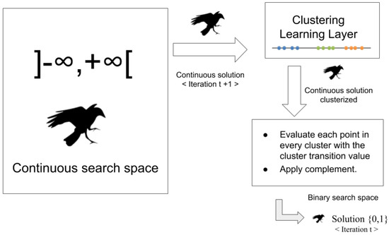
Figure 4.
Continuous to Binary KMeans.
Figure 4 shows how the real solution is clusterized and then is transformed to a binary solution applying cluster transition value using KMeans.
The third technique used is DBscan. This strategy is slightly different from previous ones because what we do is binarize the complete matrix instead of binarizing the solution vector. For that, we will create a matrix replica in its initial state (), then the metaheuristic will normally work by performing its movements in the real search space. Once each iteration is complete, the entire matrix will be clustered. As we have seen before, DBscan receives a distance () and a minimum of points (minPts) as input parameter, with this data the algorithm will only deliver a number of clusters depending on the data behavior. The following steps are performed after the clustering has been completed:
- Calculate the mean of the points to every cluster.
- Sort the clusters from least to greatest taking into account the average value of each cluster.
- Evaluate each point in the clusters by checking if a random value between 0 and 1 is equal to or greater than the average of each cluster; if it is, then we get the position and we apply the complement to the replica of the matrix (). Then the objective function is evaluated.
For this technique, we take the strategy that is illustrated in Algorithm 5. Finally, Figure 5 shows how the matrix x is clusterized and then, it is transformed to a binary matrix applying Dbscan.
| Algorithm 5: CSA + DBscan binarization technique pseudo-code |
 |
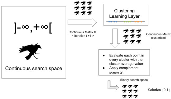
Figure 5.
Continuous to Binary DBscan.
6. Experimental Results
We propose to test our approach by solving the instances of the SCP [47] and the 0/1 Knapsack Problem [48].
6.1. Methodology
A performance analysis is totally necessary to properly evaluate the performance of metaheuristics [49]. In this study, we use the well known benchmark taken from OR-Library [50] in order to compare the given best solution of the CSA against the best known result of the benchmark. Figure 6 illustrates the steps for making an exhaustive analysis of the improved metaheuristic. For experimental design, we design aims and guidelines to demonstrate the proposed approach is a real alternative to binarization systems. Next, we establish the best value as the critical metric for evaluating future results. In this context, we apply an ordinal analysis and we employ statistical tests to determine which approach is significantly better. Finally, we describe the used hardware and software features to reproduce computational experiments, and then we report all results in tables and distribution charts.
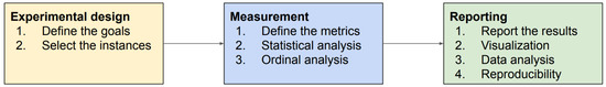
Figure 6.
Steps in performance analysis of a metaheuristic.
Moreover, it is very important to show how significant of a difference the three strategies have in this type of problem. For this reason we perform a contrast statistical test for each instance through the Kolmogorov-Smirnov-Lilliefors test to determine the independence of samples [51] and the Mann–Whitney–Wilcoxon test [52] to compare the results statistically (see Figure 7).
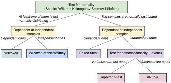
Figure 7.
Statistical significance test.
Kolmogorov-Smirnov-Lilliefors test allows us to analyze the independence of the samples by determining the or (depending if the problem is minimization or maximization) obtained from the 31 executions of each instance.
The results are evaluated using the relative percentage deviation (RPD). The RPD value quantifies the deviation of the objective value from , which is the minimal best-known value for each instance in our experiment, and it is calculated as follows:
6.2. Set Covering Problem (SCP)
The Set Covering Problem [47] is a classic combinatorial optimization problem, belonging to the NP-hard class [53], that has been applied in several real-world problems like the location of emergency facilities [3], airline and bus crew scheduling [54], vehicle scheduling [55], steel production [56], among others.
Formally, the SCP is defined as follows: let be a binary matrix with M-rows () and N-columns (), and let be a vector representing the cost of each column j, assuming that . Then, it observes that a column j covers a row i if . Therefore, it has:
The SCP consists of finding a set of elements that cover a range of needs at the lowest cost. In its matrix form, a feasible solution corresponds to a subset of columns and the needs are associated with the rows and treated as constraints. The problem aims at selecting the columns that optimally cover all the rows.
The Set Covering Problem finds a minimum cost subset S of columns such that each row is covered by at least one column of S. An integer programming formulation of the SCP is as follows:
Instances: In order to evaluate the algorithm performance when solving the SCP, we use 65 instances taken from the Beasley’s OR-library [50], which are organized in 11 sets.
Table 1 describes instance group, number of rows M, number of columns N, range of costs, density (percentage of nonzeroes in the matrix).

Table 1.
Instances taken from the Beasley’s OR-Library.
Reducing the instance size of SCP: In [57] different preprocessing methods have particularly been proposed to reduce the size of the SCP, two of them have been taken as the most effective ones, which are Column Domination and Column Inclusion; these methods are used to accelerate the processing of the algorithm.
Column Domination: It consists of eliminating the redundant columns of the problem in such a way that it does not affect the final solution.
Steps:
- All the columns are ordered according to their cost in ascending order.
- If there are equal cost columns, these are sorted in descending order by the number of rows that the column j covers.
- Verify if the column j whose rows can be covered by a set of other columns with a cost less than (cost of the column j).
- It is said that column j is dominated and can be eliminated from the problem.
Column Inclusion: If a row is covered only by one column after the domination process, it means that there is no better column to cover those rows; consequently, this column must be included in the optimal solution.
This reduction will be used as input data of instances.
6.3. Knapsack (KP)
0–1 Knapsack Problem is still an actual issue [58] which is a typical NP-hard problem in operations research. There are many studies that use this problem to prove their algorithm, such as in [59,60]. The problem may be defined as follows: given a set of objects from N, each o object has a certain weight and value. Furthermore, the number of items to be included in the collection must be determined to ensure that the full weight is less than or equal to the limit and that the full value is as large as possible.
The problem is to optimize the objective function:
Subject to:
Binary decision variables are used to indicate if item j is included in the knapsack or not. It can be assumed that all benefits and weights are positive and that all weights are smaller than capacity b.
Instances: In order to evaluate the algorithm performance of solving the KP, we used 10 instances [61].
Table 2 describes instance, dimension, and parameters: weight w, profit p, and capacity of the bag b.
Table 2.
0/1 Knapsack Problem instances.
As we can see in the instance Table 2, distinct sorts of problems are solved, each with specific sizes and values to get a wide concept of the algorithm’s behavior.
Software and Hardware: CSA was implemented in Java 1.8. The characteristics of the Personal Computer (PC) were: Windows 10 with an Intel Core i7-6700 CPU (3.4Ghz), 16 GB of RAM.
Parameter settings: Below, Table 3 shows the setup for Two-steps strategy, Table 4 shows the setup for KMeans strategy, and finally Table 5 shows setup for DBscan strategy.
Table 3.
Crow Search Algorithm (CSA) Parameters for Set Covering Problem (SCP) and Knapsack Problem (KP)—Two-steps.
Table 4.
CSA Parameters for SCP and KP—KMeans.
Table 5.
CSA Parameters for SCP and KP—DBscan.
Sixty-five instances of the SCP and ten instances of the 0/1 Knapsack Problem have been considered, which were executed 31 times each.
6.4. Comparison Results and Strategies
In [62] and in Appendix section (Appendix A.1 and Appendix A.2), we can see the results obtained; the information is detailed, also indicating each of the transfer functions and the binarization methods that were used. The data is grouped as follows: instance: name of the instance, MIN: the minimum reached value, MAX: the maximum value reached, AVG: the average value, BKS: the best known solution, RPD it is defined by the Equation (3) and finally TIME: time of execution in seconds.
As we mentioned, the first strategy implemented was Two-steps, the second strategy implemented was KMeans, and the last strategy implemented was DBscan.
Set Covering Problem Results
Comparison strategy: Table 6 shows a summary of the instances grouped by their complexity; we define three groups: G1 (easy), G2 (medium), and G3 (hard). The first group includes instances 4.1 to 6.5, the second group includes instances a.1 to d.5, and the third group includes instances nre.1 to nrh.5.
Table 6.
CSA/SCP—Two-steps vs. KMeans vs. DBscan resume summary (t.o = time out).
To get more information of the comparison between strategies, see [62]. It will easily realize how complex it is to develop all the combinations of two steps in order to get good results vs. clustering techniques.
Summary: Next, we rank the strategies in order of BKS obtained. In addition, the instances that obtained BKS in the 3 strategies are shown.
- Score
- Two-steps got 51/65 BKS.
- DBscan got 25/65 BKS.
- KMeans got 16/65 BKS.
- The three strategies got BKS in the same instances: 4.1-4.3-4.6-4.7-5.1-5.4-5.5-5.6-5.7-5.8-5.9-6.2-6.4-a.5
Instance distribution: Now that we have all the results of all the strategies that solved SCP, we compare the distribution of the samples of each instance through a box plot that shows the full distribution of the data. In order to make a summary of all the instances below, we present and describe the hardest instances of each group (4.10, 5.10, 6.5, a.5, b.5, c.5, d.5, nre.5, nrf.5, nrg.5 and nrh.5):
We can see that Figure 8 and Figure 9 are alike. The Two-steps and DBscan strategies obtained BKS but KMeans did not. However, the distribution is quite homogeneous. If we see the instance 4.10 illustrated in Figure 8, DBscan’s behavior is remarkable.
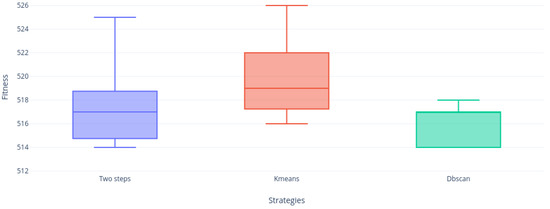
Figure 8.
Instance 4.10 distribution.
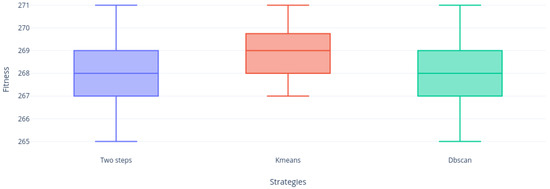
Figure 9.
Instance 5.10 distribution.
Figure 10 shows again that the Two-steps and DBscan strategies obtained BKS and the KMeans strategy did not. However, it can be appreciated again that DBscan is far more compact than Two-steps, which indicates that clustering processing is accurate in this instance. Then, Figure 11 shows us for the first time a very nice and solidly compact distribution. It is necessary to emphasize that the three strategies obtained BKS. Finally, Figure 12 shows how the Two-steps and KMeans strategies obtained BKS while DBscan did not. However, if it was very close, despite this the most compact strategies in its distribution were KMeans and DBscan.
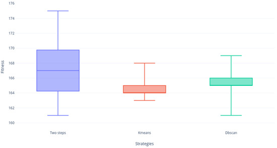
Figure 10.
Instance 6.5 distribution.
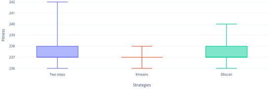
Figure 11.
Instance a.5 distribution.
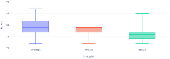
Figure 12.
Instance b.5 distribution.
If we continue analyzing the samples, we can realize that Figure 13, Figure 14, Figure 15, Figure 16 and Figure 17 are very similar, the two-step strategies and KMeans far exceeded DBscan. This gives us an indication that DBscan works better by solving small instances with this metaheuristic, perhaps due to a large number of calculations made by grouping the complete set of solutions versus KMeans that groups the solution and Two-steps that perform binarization instantly on each vector column solution.
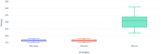
Figure 13.
Instance c.5 distribution.
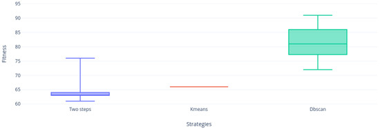
Figure 14.
Instance d.5 distribution.

Figure 15.
Instance nre.5 distribution.
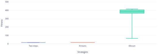
Figure 16.
Instance nrf.5 distribution.
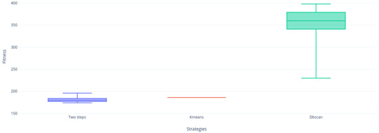
Figure 17.
Instance nrg.5 distribution.
Finally, Figure 18 show us a null contribution of DBscan, who could not complete the executions due to the excessive delay of the strategy when clustering the most difficult instances; later we can observe KMeans absolutely trapped in an optimal local. However, the Two-steps approach continues to show good results, being the most robust at the BKS level as mentioned earlier in the strategy comparison.
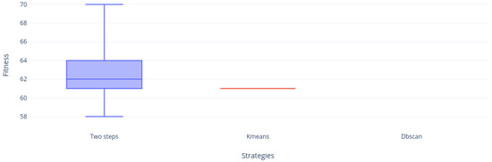
Figure 18.
Instance nrh.5 distribution.
6.5. Knapsack Problem Results
Unlike the previous problem (SCP), the Knapsack problem has fewer instances, so it was not necessary to group by complexity.
Comparison strategy: Table 7 shows a summary of the instances.
Table 7.
CSA/KP—Two-steps vs. KMeans vs. DBscan resume summary.
To get more information of the comparison between strategies, see [62].
Summary: Next, we rank the strategies in order of BKS obtained. In addition, the instances that obtained BKS in the three strategies are shown.
- Score
- -
- Two-steps got 6/10 BKS.
- -
- DBscan got 5/10 BKS.
- -
- KMeans got 4/10 BKS.
- The three strategies got BKS in the same instances: f3-f4-f7-f9
Instance distribution: Now that we have all the results of all the strategies that KP solved, we compare the distribution of the samples of each instance through a box diagram that shows the complete distribution of the data. To summarize all the instances below, we present and describe instances where the optimum was not reached because instances f3, f4, f7, and f9 always obtain BKS in each execution with the three strategies, so it is not necessary to graph these instances.
Figure 19, Figure 20, Figure 21, Figure 22, Figure 23 and Figure 24 shows us that the Two-steps strategy achieved better results but DBscan strategy is far more compact than KMeans strategy. Figure 24 shows the only instance where DBscan did not win to KMeans.
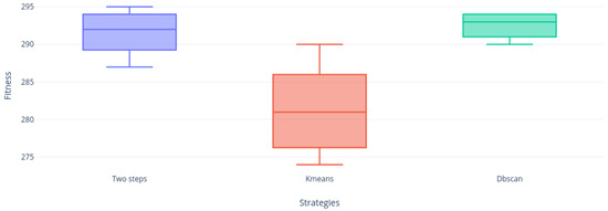
Figure 19.
Instance f1 distribution.
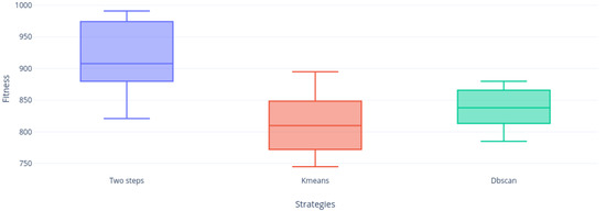
Figure 20.
Instance f2 distribution.
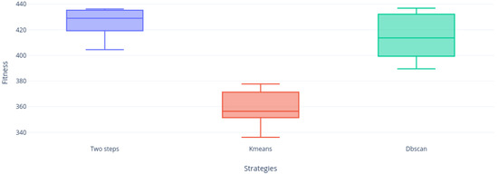
Figure 21.
Instance f5 distribution.
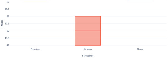
Figure 22.
Instance f6 distribution.
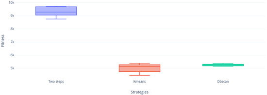
Figure 23.
Instance f8 distribution.
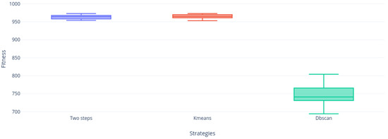
Figure 24.
Instance f10 distribution.
7. Statistical Test
As we mentioned, in order to determine independence, we propose the following hypotheses:
- -
- : states that / follows a normal distribution.
- -
- : states the opposite.
The test performed has yielded lower than ; therefore, cannot be assumed. Now that we know that the samples are independent and it cannot be assumed that they follow a normal distribution, it is not feasible to use the central limit theorem. Therefore, for evaluating the heterogeneity of samples we use a nonparametric evaluation called Mann–Whitney–Wilcoxon test. To compare all the results of the hardest instances, we propose the following hypotheses:
- -
- : Two-steps is better than KMeans
- -
- : states the opposite.
- -
- : Two-steps is better than DBscan
- -
- : states the opposite.
- -
- : KMeans is better than DBscan
- -
- : states the opposite.
Finally, the contrast statistical test demonstrates which technique is significantly better.
Table 8, Table 9, Table 10, Table 11, Table 12, Table 13, Table 14, Table 15, Table 16, Table 17, Table 18, Table 19, Table 20, Table 21, Table 22, Table 23 and Table 24 compare SCP and 0/1 KP binariztion strategies for the hardest instances tested via the Wilcoxon’s signed rank test. As the significance level is also established to , smaller values than defines that , , and cannot be assumed.
Table 8.
p-values for instance 4.10.
Table 9.
p-values for instance 5.10.
Table 10.
p-values for instance 6.5.
Table 11.
p-values for instance a.5.
Table 12.
p-values for instance b.5.
Table 13.
p-values for instance c.5.
Table 14.
p-values for instance d.5.
Table 15.
p-values for instance nre.5.
Table 16.
p-values for instance nrf.5.
Table 17.
p-values for instance nrg.5.
Table 18.
p-values for instance nrh.5.
Table 19.
p-values for instance f.1.
Table 20.
p-values for instance f.2.
Table 21.
p-values for instance f.5.
Table 22.
p-values for instance f.6.
Table 23.
p-values for instance f.8.
Table 24.
p-values for instance f.10.
We have a method belonging to the PISA system to conduct the test run that supports the study. To this method, we indicate all data distributions (each in a file and each data in a line) and the algorithm will give us a p-value for the hypotheses.
The following tables show the result of the Mann-Whitney-Wilcoxon test. To understand them, it is necessary to have knowledge of the following acronyms:
- SWS = Statistically without significance.
- D/A = Does not apply.
SCP—p-value
KP—p-value
All reported p-values are less than 0.05; as indicated above, SWS indicates that it has no statistical significance, and D/A indicates that the comparison cannot be done because one of the strategies does not contain any data. So, with this information, we can clearly see which strategy was better than the three in each instance reported. As a resume for results for the SCP p-values lower than 0.05 were 10 for Two-steps, 10 for KMeans, and 5 for DBscan. On the other hand, results for the 0/1 KP p-values lower than 0.05 were 0 for Two steps, 10 for KMeans, and 5 for DBscan.
8. Conclusions
After implementing and analyzing binarization strategies through clusters, we can realize that DBscan achieved better results than KMeans at the BKS level. However, the execution times of DBscan were longer than KMeans; we believe that this has a clear explanation. The way in which the experiment was developed with clustering is crucial; KMeans cluster a vector while the BDscan clusters the complete matrix, which makes this technique take longer. Moreover, we do not report the solving time results due to the fact that it is known that this measure basically depends of the characteristics of the used machine (computer). Finally, our work is focused on enhancing the binariazation process for metahuerisics in order to find better results. In this way, we certainly have sacrificed the solving time but we think that DBscan is very promising because with these experiments we can realize that although we cluster the complete matrix with this technique, which took more time to execute, it still obtained good results.
When solving SCP, we have tested 65 nonunique instances of the Beasley OR Library and 10 well-known instances to solve KP, where classical technique obtained better results than clustering techniques in both problems. We believe that due to the number of combinations made (992 experiments for Two-steps), it allows a better performance on this metahuristic and also that it is necessary to make adjustments, perhaps of autonomous search on the clustering techniques to obtain a better performance.
The best results were obtained with the S-Shape transfer functions (S-Shape 4 predominates over the others) and Elitist binarization method. The worst results were the combination of the V-Shape transfer function with the binarization complement. It is very relevant to say that KMeans did not got better results than Two-steps strategy. On the other hand, it is relevant that DBscan obtained good results, better than KMeans and worse than Two-steps but the quantity of Two-step combinations is a very influential factor since with 32 different different ways of binarization it is far from being an easy way to implement; this requires time and knowledge of an expert user. Which means we reduce to one single experiment (31 executions) with DBscan over the combinatorial strategies of two-step getting good results. Statistically DBscan got better performance.
As future work, we plan to reverse the strategies of KMeans and DBscan by solving the grouping problem as a matrix with KMeans and as a unique solution with DBscan. In addition, we will implement a self-adaptive approach to get better results. Finally, we will apply the online control parameters in the Two-steps strategy to reach BKS in instances that did not reach optimal values.
Author Contributions
Formal analysis, S.V.; investigation, R.S., B.C., S.V., N.C. and R.O.; methodology, R.S. and B.C.; resources, R.S. and B.C.; software, R.O., S.V. and N.C.; validation, R.O., S.V., F.P., C.C. and N.C.; writing—original draft, S.V.; writing—review and editing, R.S., R.O. and S.V. All the authors of this paper hold responsibility for every part of this manuscript. All authors have read and agreed to the published version of the manuscript.
Funding
Ricardo Soto is supported by Grant CONICYT/FONDECYT/REGULAR/1190129. B.C. is supported by Grant CONICYT/FONDECYT/REGULAR/1171243. Nicolás Caselli is supported by PUCV-INF 2019.
Conflicts of Interest
The authors declare no conflict of interest. The founding sponsors had no role in the design of the study; in the collection, analyses, or interpretation of data; in the writing of the manuscript, and in the decision to publish the results.
Appendix A
Appendix A.1. Set Covering Problem Results
Appendix A.1.1. SCP—Crow Search Algorithm
Table A1.
CSA/SCP—SShape 1—Two-steps vs. KMeans vs. DBscan (t.o = time out).
Table A1.
CSA/SCP—SShape 1—Two-steps vs. KMeans vs. DBscan (t.o = time out).
| Instance | BKS | S1+Stand. | S1+Comp. | S1+Static | S1+Elitist | KMeans | DBscan | ||||||
|---|---|---|---|---|---|---|---|---|---|---|---|---|---|
| MIN | AVG | MIN | AVG | MIN | AVG | MIN | AVG | MIN | AVG | MIN | AVG | ||
| 4.1 | 429 | 438 | 444.81 | 459 | 463.32 | 465 | 494.87 | 432 | 443.74 | 429 | 430 | 429 | 430.38 |
| 4.2 | 512 | 522 | 550.35 | 579 | 586.39 | 612 | 698.06 | 528 | 551.10 | 513 | 515.84 | 512 | 514.77 |
| 4.3 | 516 | 520 | 532.58 | 552 | 564.19 | 587 | 620.47 | 564 | 578.36 | 516 | 520.61 | 516 | 518.87 |
| 4.4 | 494 | 513 | 524.58 | 544 | 555.26 | 566 | 620.13 | 496 | 515.84 | 495 | 498.87 | 494 | 496.10 |
| 4.5 | 512 | 518 | 529.23 | 554 | 570.45 | 601 | 680.39 | 518 | 529.55 | 514 | 514.90 | 512 | 513.23 |
| 4.6 | 560 | 577 | 590.23 | 614 | 626.23 | 661 | 798.55 | 566 | 590 | 560 | 562.35 | 560 | 560.19 |
| 4.7 | 430 | 436 | 445.90 | 485 | 492.81 | 498 | 558.90 | 438 | 451.68 | 430 | 432.26 | 430 | 430.81 |
| 4.8 | 492 | 501 | 513.74 | 532 | 540.29 | 585 | 680.61 | 499 | 508.52 | 493 | 496.13 | 492 | 494.10 |
| 4.9 | 641 | 675 | 690.42 | 722 | 745.06 | 807 | 911.65 | 657 | 687.94 | 645 | 657.90 | 641 | 647.50 |
| 4.10 | 514 | 534 | 554.74 | 569 | 578.90 | 595 | 678.27 | 528 | 550.23 | 516 | 519.9 | 514 | 515.81 |
| 5.1 | 253 | 265 | 275.29 | 291 | 296.26 | 309 | 352.61 | 258 | 271.32 | 253 | 255.74 | 253 | 255.52 |
| 5.2 | 302 | 310 | 327.55 | 352 | 363.68 | 421 | 471.19 | 317 | 326.74 | 308 | 309.81 | 302 | 306.68 |
| 5.3 | 226 | 230 | 240.19 | 249 | 252.65 | 278 | 310.35 | 229 | 239.74 | 228 | 228.68 | 226 | 227.32 |
| 5.4 | 242 | 242 | 249.43 | 263 | 264.90 | 301 | 354.12 | 254 | 269.84 | 242 | 242.23 | 242 | 243.29 |
| 5.5 | 211 | 211 | 223.13 | 242 | 245.97 | 247 | 301.87 | 245 | 268.21 | 211 | 212.03 | 211 | 213.90 |
| 5.6 | 213 | 222 | 235.71 | 251 | 254.39 | 267 | 309.87 | 226 | 237.87 | 213 | 215.10 | 213 | 213.04 |
| 5.7 | 293 | 305 | 314.61 | 327 | 335.29 | 360 | 408.94 | 305 | 315.10 | 293 | 297.68 | 293 | 295.35 |
| 5.8 | 288 | 302 | 310.06 | 342 | 348.48 | 370 | 424.65 | 299 | 310.84 | 288 | 290.35 | 288 | 290.39 |
| 5.9 | 279 | 283 | 303.23 | 321 | 331.29 | 357 | 381.28 | 287 | 305.68 | 279 | 280.52 | 279 | 279.90 |
| 5.10 | 265 | 271 | 277.45 | 294 | 298.45 | 335 | 376.16 | 273 | 277.10 | 267 | 268.77 | 265 | 267.97 |
| 6.1 | 138 | 146 | 152.03 | 159 | 166 | 210 | 287.13 | 145 | 151.71 | 140 | 142.90 | 140 | 143.42 |
| 6.2 | 146 | 152 | 157.29 | 163 | 169 | 308 | 401.10 | 150 | 156.10 | 146 | 148.87 | 146 | 149.71 |
| 6.3 | 154 | 148 | 156.52 | 162 | 167.23 | 268 | 379.39 | 148 | 156.65 | 147 | 148.16 | 145 | 149.65 |
| 6.4 | 131 | 131 | 138.26 | 137 | 141.94 | 247 | 359.87 | 138 | 147.64 | 131 | 131.68 | 131 | 133.03 |
| 6.5 | 161 | 171 | 181.35 | 186 | 194.50 | 267 | 419.94 | 173 | 181.42 | 163 | 164.68 | 162 | 165.39 |
| AVG | 336.08 | 344.92 | 356.75 | 373.96 | 382.11 | 420.88 | 491.21 | 346.92 | 360.91 | 336.80 | 339.43 | 335.84 | 346.80 |
| a.1 | 253 | 257 | 263.74 | 269 | 272.48 | 474 | 584.81 | 256 | 261.81 | 254 | 255.55 | 254 | 256 |
| a.2 | 252 | 262 | 274.42 | 300 | 305.23 | 439 | 565.55 | 267 | 274.74 | 257 | 259.48 | 256 | 260.65 |
| a.3 | 232 | 242 | 251 | 256 | 258.16 | 410 | 525.81 | 242 | 250.35 | 235 | 237.10 | 233 | 237.35 |
| a.4 | 234 | 239 | 250.71 | 264 | 268.35 | 409 | 523.32 | 236 | 250.97 | 235 | 237.39 | 236 | 239.97 |
| a.5 | 236 | 239 | 243.32 | 258 | 263.03 | 421 | 540.65 | 238 | 241.84 | 236 | 237.06 | 236 | 237.52 |
| b.1 | 69 | 75 | 81.61 | 82 | 86.10 | 347 | 518.13 | 72 | 81.58 | 74 | 79.61 | 69 | 76.48 |
| b.2 | 76 | 84 | 90.26 | 92 | 94.19 | 411 | 549.61 | 81 | 88.35 | 83 | 90.03 | 81 | 86.81 |
| b.3 | 80 | 80 | 85.94 | 91 | 91.90 | 507 | 535.9 | 85 | 87.65 | 84 | 88.55 | 82 | 88.81 |
| b.4 | 79 | 83 | 89.10 | 96 | 100.26 | 517 | 660.52 | 84 | 88.55 | 84 | 87.90 | 83 | 88.16 |
| b.5 | 72 | 72 | 78.92 | 82 | 84.55 | 498 | 587.58 | 76 | 80.35 | 72 | 77.68 | 78 | 76.03 |
| c.1 | 227 | 232 | 237.65 | 263 | 264.65 | 512 | 718.52 | 233 | 236.71 | 228 | 230.29 | 233 | 238.77 |
| c.2 | 219 | 228 | 236.61 | 259 | 263.13 | 617 | 782.81 | 226 | 235.58 | 226 | 222.71 | 226 | 232.74 |
| c.3 | 243 | 257 | 270.55 | 297 | 302.32 | 738 | 939.94 | 261 | 271 | 254 | 256.68 | 253 | 264 |
| c.4 | 219 | 231 | 243.45 | 256 | 260.17 | 618 | 783.23 | 233 | 243.58 | 225 | 227.97 | 224 | 233.10 |
| c.5 | 215 | 219 | 226.81 | 245 | 250.29 | 529 | 713.77 | 218 | 226.06 | 215 | 216.35 | 222 | 230.42 |
| d.1 | 60 | 61 | 68.29 | 70 | 70.87 | 600 | 889.42 | 63 | 67.23 | 66 | 66 | 68 | 79.65 |
| d.2 | 66 | 70 | 73.52 | 77 | 78.68 | 686 | 1001.55 | 68 | 74.19 | 71 | 71 | 73 | 89.71 |
| d.3 | 72 | 77 | 81.68 | 83 | 86.74 | 881 | 1114.29 | 78 | 82.13 | 82 | 82 | 82 | 100.84 |
| d.4 | 66 | 65 | 68.29 | 71 | 71.81 | 644 | 945 | 65 | 68.23 | 67 | 67 | 70 | 81.74 |
| d.5 | 61 | 64 | 67.74 | 69 | 69.97 | 631 | 909.13 | 63 | 67.39 | 66 | 66 | 72 | 81.29 |
| AVG | 151.55 | 156.85 | 164.18 | 174 | 177.14 | 544.45 | 719.47 | 157.25 | 163.91 | 155.70 | 157.81 | 156.55 | 164 |
| nre.1 | 29 | 30 | 33.23 | 32 | 33 | 1354 | 1643.54 | 30 | 32.68 | 30 | 30 | 70 | 80.03 |
| nre.2 | 30 | 33 | 37.45 | 36 | 37.61 | 1405 | 1732.55 | 33 | 36.19 | 34 | 34 | 83 | 128.32 |
| nre.3 | 27 | 28 | 33.61 | 32 | 34.61 | 1137 | 1416.77 | 30 | 33.61 | 34 | 34 | 74 | 112.35 |
| nre.4 | 28 | 31 | 34 | 34 | 34 | 1210 | 1712.48 | 30 | 33.90 | 33 | 34 | 83 | 177.45 |
| nre.5 | 28 | 30 | 32.94 | 33 | 33.87 | 1292 | 1860.23 | 30 | 32.77 | 30 | 30 | 92 | 150.52 |
| nrf.1 | 14 | 17 | 19 | 17 | 17.03 | 667 | 903.48 | 15 | 18.42 | 17 | 17 | 372 | 444.19 |
| nrf.2 | 15 | 16 | 18.71 | 18 | 18 | 607 | 836.29 | 16 | 18.61 | 18 | 18 | 74 | 404.58 |
| nrf.3 | 14 | 17 | 19.39 | 19 | 19.90 | 858 | 1034.90 | 17 | 19.29 | 19 | 19 | 335 | 487.25 |
| nrf.4 | 14 | 15 | 18.45 | 17 | 18.61 | 667 | 902.97 | 16 | 18.29 | 18 | 18 | 52 | 420.52 |
| nrf.5 | 13 | 15 | 18.29 | 16 | 16.32 | 653 | 844.23 | 15 | 17.61 | 16 | 16 | 65 | 371.03 |
| nrg.1 | 176 | 201 | 208.26 | 230 | 233.48 | 4473 | 5588.65 | 192 | 203.39 | 197 | 197 | 287 | 385.13 |
| nrg.2 | 154 | 172 | 181.06 | 187 | 190.48 | 3848 | 4648.48 | 166 | 174.16 | 168 | 168 | 208 | 284.29 |
| nrg.3 | 166 | 180 | 190.55 | 196 | 197.84 | 4319 | 5026.55 | 180 | 185.19 | 183 | 183 | 211 | 347.23 |
| nrg.4 | 168 | 187 | 200.03 | 216 | 219.26 | 4142 | 4935.29 | 180 | 192.10 | 186 | 186 | 250 | 345.77 |
| nrg.5 | 168 | 191 | 201.10 | 213 | 217.32 | 4198 | 5155 | 181 | 193.84 | 186 | 186 | 230 | 353.97 |
| nrh.1 | 63 | 102 | 124.68 | 82 | 83.65 | 9080 | 10,028.42 | 72 | 77.42 | 77 | 77 | t.o. | t.o. |
| nrh.2 | 63 | 92 | 120.10 | 81 | 81.81 | 9085 | 10,332.71 | 71 | 76.48 | 71 | 71 | t.o. | t.o. |
| nrh.3 | 59 | 89 | 120.23 | 74 | 75 | 8101 | 9886.68 | 67 | 73.61 | 69 | 69 | t.o. | t.o. |
| nrh.4 | 58 | 91 | 116.52 | 73 | 74.97 | 8592 | 9899.26 | 67 | 70.94 | 68 | 68 | t.o. | t.o. |
| nrh.5 | 55 | 88 | 105.13 | 68 | 68.74 | 7786 | 9318.55 | 62 | 67.16 | 61 | 61 | t.o. | t.o. |
| AVG | 67.10 | 81.25 | 91.63 | 83.70 | 85.27 | 3673.70 | 4385.35 | 73.50 | 78.78 | 75.75 | 75.80 | t.o. | t.o. |
Table A2.
CSA/SCP—SShape 2—Two-steps vs. KMeans vs. DBscan (t.o = time out).
Table A2.
CSA/SCP—SShape 2—Two-steps vs. KMeans vs. DBscan (t.o = time out).
| Instance | BKS | S2+Stand. | S2+Comp. | S2+Static | S2+Elitist | KMeans | DBscan | ||||||
|---|---|---|---|---|---|---|---|---|---|---|---|---|---|
| MIN | AVG | MIN | AVG | MIN | AVG | MIN | AVG | MIN | AVG | MIN | AVG | ||
| 4.1 | 429 | 432 | 443.48 | 457 | 462.81 | 622 | 686.58 | 431 | 439.73 | 429 | 430 | 429 | 430.38 |
| 4.2 | 512 | 517 | 549.26 | 578 | 587.26 | 929 | 1084.16 | 522 | 549.50 | 513 | 515.84 | 512 | 514.77 |
| 4.3 | 516 | 519 | 532 | 555 | 564.23 | 789 | 987.25 | 578 | 687.47 | 516 | 520.61 | 516 | 518.87 |
| 4.4 | 494 | 500 | 520.55 | 542 | 555.81 | 861 | 963.39 | 501 | 517.03 | 495 | 498.87 | 494 | 496.10 |
| 4.5 | 512 | 518 | 531.84 | 557 | 573.48 | 901 | 1101.97 | 514 | 529.40 | 514 | 514.90 | 512 | 513.23 |
| 4.6 | 560 | 566 | 588.48 | 610 | 624.81 | 1194 | 1320.35 | 568 | 588.70 | 560 | 562.35 | 560 | 560.19 |
| 4.7 | 430 | 436 | 447.13 | 479 | 491.35 | 821 | 892.06 | 437 | 448.60 | 430 | 432.26 | 430 | 430.81 |
| 4.8 | 492 | 499 | 514.74 | 525 | 539.52 | 946 | 1095.10 | 493 | 506.97 | 493 | 496.13 | 492 | 494.10 |
| 4.9 | 641 | 641 | 652.16 | 722 | 743.39 | 1368 | 1499.48 | 662 | 682.20 | 645 | 657.90 | 641 | 647.50 |
| 4.10 | 514 | 523 | 550.52 | 560 | 575.35 | 873 | 1064.16 | 518 | 546.53 | 516 | 519.9 | 514 | 515.81 |
| 5.1 | 253 | 257 | 273.52 | 287 | 295.26 | 490 | 556.81 | 260 | 270.27 | 253 | 255.74 | 253 | 255.52 |
| 5.2 | 302 | 312 | 325.23 | 352 | 361.77 | 717 | 800.55 | 308 | 321.53 | 308 | 309.81 | 302 | 306.68 |
| 5.3 | 226 | 231 | 240.77 | 250 | 253.23 | 466 | 522.19 | 229 | 237.13 | 228 | 228.68 | 226 | 227.32 |
| 5.4 | 242 | 244 | 249.13 | 261 | 264.68 | 357 | 487.25 | 247 | 278.64 | 242 | 242.23 | 242 | 243.29 |
| 5.5 | 211 | 215 | 223.77 | 242 | 245.87 | 287 | 359.25 | 287 | 301.07 | 211 | 212.03 | 211 | 213.90 |
| 5.6 | 213 | 217 | 235.61 | 245 | 253.68 | 422 | 498.10 | 224 | 234 | 213 | 215.10 | 213 | 213.04 |
| 5.7 | 293 | 307 | 312.90 | 331 | 334.16 | 563 | 650.16 | 299 | 311.40 | 293 | 297.68 | 293 | 295.35 |
| 5.8 | 288 | 291 | 310.71 | 339 | 346.74 | 575 | 654.52 | 298 | 308.57 | 288 | 290.35 | 288 | 290.39 |
| 5.9 | 279 | 288 | 306.16 | 320 | 331.23 | 487 | 587.37 | 297 | 357.26 | 279 | 280.52 | 279 | 279.90 |
| 5.10 | 265 | 269 | 276.58 | 290 | 297.55 | 553 | 609.87 | 272 | 278 | 267 | 268.77 | 265 | 267.97 |
| 6.1 | 138 | 148 | 151.67 | 161 | 165.26 | 569 | 732.77 | 143 | 150.77 | 140 | 142.90 | 140 | 143.42 |
| 6.2 | 146 | 150 | 158.58 | 166 | 169 | 774 | 995.52 | 151 | 157.90 | 146 | 148.87 | 146 | 149.71 |
| 6.3 | 154 | 150 | 157.65 | 162 | 167.77 | 766 | 949.35 | 150 | 155.27 | 147 | 148.16 | 145 | 149.65 |
| 6.4 | 131 | 134 | 138.65 | 139 | 142.06 | 778 | 954.21 | 147 | 157.28 | 131 | 131.68 | 131 | 133.03 |
| 6.5 | 161 | 175 | 181.94 | 186 | 192.58 | 792 | 1000.87 | 170 | 179.47 | 163 | 164.68 | 162 | 165.39 |
| AVG | 336.08 | 341.56 | 354.92 | 372.64 | 381.55 | 716 | 842.13 | 348.24 | 367.78 | 336.80 | 339.43 | 335.84 | 338.25 |
| a.1 | 253 | 258 | 264.39 | 270 | 273.16 | 981 | 1126.26 | 257 | 262.60 | 254 | 255.55 | 254 | 256 |
| a.2 | 252 | 263 | 275.06 | 301 | 305.32 | 943 | 1066.48 | 266 | 274.33 | 257 | 259.48 | 256 | 260.65 |
| a.3 | 232 | 247 | 250.35 | 256 | 257.87 | 812 | 998.84 | 241 | 250.03 | 235 | 237.10 | 233 | 237.35 |
| a.4 | 234 | 234 | 240.06 | 265 | 268.90 | 848 | 977.29 | 241 | 251.03 | 235 | 237.39 | 236 | 239.97 |
| a.5 | 236 | 238 | 244.26 | 259 | 264.29 | 834 | 971.19 | 239 | 242.90 | 236 | 237.06 | 236 | 237.52 |
| b.1 | 69 | 72 | 80.58 | 82 | 85.26 | 1068 | 1196.61 | 76 | 80.83 | 74 | 79.61 | 69 | 76.48 |
| b.2 | 76 | 76 | 81.45 | 93 | 94 | 1039 | 1179.84 | 80 | 88.30 | 83 | 90.03 | 81 | 86.81 |
| b.3 | 80 | 82 | 86.55 | 91 | 91.84 | 1054 | 1178.89 | 86 | 91.04 | 84 | 88.55 | 82 | 88.81 |
| b.4 | 79 | 84 | 88.68 | 95 | 100.23 | 1153 | 1353.97 | 83 | 87.57 | 84 | 87.90 | 83 | 88.16 |
| b.5 | 72 | 73 | 79.55 | 82 | 84.52 | 1127 | 1201.31 | 78 | 84.89 | 72 | 77.68 | 78 | 76.03 |
| c.1 | 227 | 233 | 240.23 | 262 | 264.68 | 1128 | 1308.87 | 230 | 236.47 | 228 | 230.29 | 233 | 238.77 |
| c.2 | 219 | 219 | 2225.10 | 254 | 262.68 | 1359 | 1470.74 | 230 | 237.47 | 226 | 222.71 | 226 | 232.74 |
| c.3 | 243 | 260 | 272.03 | 295 | 301.52 | 1447 | 1734.35 | 259 | 269.80 | 254 | 256.68 | 253 | 264 |
| c.4 | 219 | 235 | 243.74 | 254 | 259.42 | 1365 | 1463.19 | 233 | 243.40 | 225 | 227.97 | 224 | 233.10 |
| c.5 | 215 | 219 | 225.65 | 246 | 249.77 | 1253 | 1364.74 | 219 | 225.50 | 215 | 216.35 | 222 | 230.42 |
| d.1 | 60 | 63 | 68.77 | 70 | 70.87 | 1483 | 1682.68 | 62 | 67.67 | 66 | 66 | 68 | 79.65 |
| d.2 | 66 | 69 | 74.45 | 77 | 78.23 | 1608 | 1893.90 | 69 | 73.57 | 71 | 71 | 73 | 89.71 |
| d.3 | 72 | 78 | 82.06 | 83 | 86.68 | 1900 | 2102.94 | 77 | 80.40 | 82 | 82 | 82 | 100.84 |
| d.4 | 66 | 64 | 68.65 | 70 | 71.81 | 1531 | 1698.81 | 64 | 68.27 | 67 | 67 | 70 | 81.74 |
| d.5 | 61 | 62 | 67.94 | 69 | 69.90 | 1521 | 1699.13 | 64 | 66.87 | 66 | 66 | 72 | 81.29 |
| AVG | 151.55 | 156.45 | 262.97 | 173.70 | 177.05 | 1222.70 | 1383.50 | 157.70 | 164.15 | 155.70 | 157.81 | 156.55 | 164 |
| nre.1 | 29 | 29 | 33.14 | 32 | 33 | 2147 | 2147.65 | 30 | 33.85 | 30 | 30 | 70 | 80.03 |
| nre.2 | 30 | 32 | 37.29 | 36 | 37.61 | 2652 | 2897.61 | 33 | 37 | 34 | 34 | 83 | 128.32 |
| nre.3 | 27 | 31 | 34.23 | 33 | 34.52 | 2242 | 2510.84 | 30 | 33.20 | 34 | 34 | 74 | 112.35 |
| nre.4 | 28 | 29 | 34.32 | 33 | 33.97 | 2519 | 2804.13 | 31 | 33.97 | 33 | 34 | 83 | 177.45 |
| nre.5 | 28 | 30 | 33.58 | 33 | 33.94 | 2697 | 2965.90 | 29 | 32.67 | 30 | 30 | 92 | 150.52 |
| nrf.1 | 14 | 16 | 18.16 | 17 | 17 | 1438 | 1688.13 | 16 | 18.53 | 17 | 17 | 372 | 444.19 |
| nrf.2 | 15 | 16 | 19.23 | 17 | 17.97 | 1335 | 1516.13 | 17 | 18.47 | 18 | 18 | 74 | 404.58 |
| nrf.3 | 14 | 17 | 19.77 | 19 | 19.87 | 1540 | 1825.87 | 17 | 19.50 | 19 | 19 | 335 | 487.25 |
| nrf.4 | 14 | 16 | 18.68 | 17 | 18.71 | 1524 | 1664.94 | 16 | 18.37 | 18 | 18 | 52 | 420.52 |
| nrf.5 | 13 | 16 | 18.10 | 16 | 16.32 | 1313 | 1445.74 | 15 | 17.83 | 16 | 16 | 65 | 371.03 |
| nrg.1 | 176 | 327 | 371.45 | 230 | 233.13 | 7127 | 7506.23 | 192 | 203.50 | 197 | 197 | 287 | 385.13 |
| nrg.2 | 154 | 233 | 279.13 | 185 | 189.77 | 5994 | 6340.61 | 167 | 175.87 | 168 | 168 | 208 | 284.29 |
| nrg.3 | 166 | 281 | 315.81 | 195 | 197.71 | 6580 | 6997.29 | 178 | 186.17 | 183 | 183 | 211 | 347.23 |
| nrg.4 | 168 | 272 | 303.65 | 215 | 218.90 | 6601 | 7007.48 | 183 | 192.27 | 186 | 186 | 250 | 345.77 |
| nrg.5 | 168 | 276 | 329 | 216 | 217.55 | 6778 | 7198.52 | 184 | 194.33 | 186 | 186 | 230 | 353.97 |
| nrh.1 | 63 | 1165 | 1405.97 | 83 | 83.77 | 12,353 | 12,926.58 | 72 | 77.97 | 71 | 71 | t.o. | t.o. |
| nrh.2 | 63 | 1153 | 1326.81 | 79 | 81.77 | 11,778 | 12,818.74 | 73 | 78.57 | 71 | 71 | t.o. | t.o. |
| nrh.3 | 59 | 1199 | 1361.74 | 74 | 74.87 | 11,992 | 12,604.52 | 69 | 73.53 | 69 | 69 | t.o. | t.o. |
| nrh.4 | 58 | 1187 | 1334.77 | 73 | 74.84 | 12,295 | 12,797.39 | 66 | 71.03 | 68 | 68 | t.o. | t.o. |
| nrh.5 | 55 | 1011 | 1181.94 | 67 | 68.71 | 11,477 | 12,064.84 | 63 | 68.87 | 61 | 61 | t.o. | t.o. |
| AVG | 67.10 | 366.80 | 423.83 | 83.50 | 85.19 | 5619.10 | 5986.45 | 74.05 | 79.27 | 75.45 | 75.50 | t.o. | t.o. |
Table A3.
CSA/SCP—SShape 3—Two-steps vs. KMeans vs. DBscan (t.o = time out).
Table A3.
CSA/SCP—SShape 3—Two-steps vs. KMeans vs. DBscan (t.o = time out).
| Instance | BKS | S3+Stand. | S3+Comp. | S3+Static | S3+Elitist | KMeans | DBscan | ||||||
|---|---|---|---|---|---|---|---|---|---|---|---|---|---|
| MIN | AVG | MIN | AVG | MIN | AVG | MIN | AVG | MIN | AVG | MIN | AVG | ||
| 4.1 | 429 | 431 | 442.52 | 452 | 461.10 | 587 | 667.32 | 432 | 439.45 | 429 | 430 | 429 | 430.38 |
| 4.2 | 512 | 515 | 542.26 | 576 | 585.35 | 906 | 1028.52 | 515 | 545.26 | 513 | 515.84 | 512 | 514.77 |
| 4.3 | 516 | 516 | 529.13 | 554 | 564.97 | 798 | 869.54 | 579 | 602.32 | 516 | 520.61 | 516 | 518.87 |
| 4.4 | 494 | 495 | 518.71 | 544 | 553.81 | 828 | 914.39 | 501 | 513.42 | 495 | 498.87 | 494 | 496.10 |
| 4.5 | 512 | 517 | 527.61 | 559 | 568.74 | 863 | 1036 | 514 | 525.35 | 514 | 514.90 | 512 | 513.23 |
| 4.6 | 560 | 565 | 585.53 | 618 | 624.13 | 1082 | 1239.10 | 566 | 587.68 | 560 | 562.35 | 560 | 560.19 |
| 4.7 | 430 | 434 | 445.52 | 484 | 491.16 | 728 | 830.16 | 438 | 447 | 430 | 432.26 | 430 | 430.81 |
| 4.8 | 492 | 498 | 508.68 | 529 | 539.26 | 942 | 1075.97 | 497 | 506.26 | 493 | 496.13 | 492 | 494.10 |
| 4.9 | 641 | 654 | 684.03 | 726 | 741.90 | 1145 | 1399.77 | 656 | 677.03 | 645 | 657.90 | 641 | 647.50 |
| 4.10 | 514 | 518 | 540.97 | 568 | 578.26 | 852 | 1017.61 | 517 | 537.58 | 516 | 519.9 | 514 | 515.81 |
| 5.1 | 253 | 260 | 270.84 | 289 | 294.16 | 471 | 519.52 | 257 | 268.13 | 253 | 255.74 | 253 | 255.52 |
| 5.2 | 302 | 313 | 325.77 | 349 | 360.81 | 694 | 761.77 | 314 | 323.06 | 308 | 309.81 | 302 | 306.68 |
| 5.3 | 226 | 229 | 237 | 249 | 252.81 | 419 | 476.16 | 228 | 234.52 | 228 | 228.68 | 226 | 227.32 |
| 5.4 | 242 | 243 | 248.53 | 261 | 264.45 | 368 | 589.12 | 302 | 317.22 | 242 | 242.23 | 242 | 243.29 |
| 5.5 | 211 | 214 | 221.10 | 241 | 244.97 | 358 | 475.74 | 235 | 247.54 | 211 | 212.03 | 211 | 213.90 |
| 5.6 | 213 | 221 | 233.32 | 250 | 253.84 | 383 | 469.61 | 222 | 234 | 213 | 215.10 | 213 | 213.04 |
| 5.7 | 293 | 301 | 311.84 | 327 | 332.84 | 558 | 622.35 | 302 | 311.52 | 293 | 297.68 | 293 | 295.35 |
| 5.8 | 288 | 298 | 307.87 | 338 | 345.74 | 545 | 631.48 | 294 | 307.29 | 288 | 290.35 | 288 | 290.39 |
| 5.9 | 279 | 281 | 303.13 | 315 | 329.26 | 4412 | 506.06 | 301 | 387.31 | 279 | 280.52 | 279 | 279.90 |
| 5.10 | 265 | 271 | 276.39 | 294 | 297.97 | 497 | 573.84 | 268 | 275.19 | 267 | 268.77 | 265 | 267.97 |
| 6.1 | 138 | 145 | 151.55 | 159 | 164.97 | 701 | 874.98 | 144 | 148.90 | 140 | 142.90 | 140 | 143.42 |
| 6.2 | 146 | 151 | 157.61 | 166 | 169.19 | 803 | 941.94 | 148 | 156.29 | 146 | 148.87 | 146 | 149.71 |
| 6.3 | 154 | 148 | 155.68 | 160 | 166.71 | 788 | 892.10 | 148 | 152.84 | 147 | 148.16 | 145 | 149.65 |
| 6.4 | 131 | 132 | 137 | 139 | 141.81 | 814 | 912.32 | 139 | 150.01 | 131 | 131.68 | 131 | 133.03 |
| 6.5 | 161 | 170 | 180.42 | 183 | 192 | 816 | 916.68 | 165 | 177.97 | 163 | 164.68 | 162 | 165.39 |
| AVG | 336.08 | 340.80 | 353.72 | 373.20 | 380.81 | 854.32 | 809.68 | 347.28 | 362.93 | 336.80 | 339.44 | 335.84 | 338.25 |
| a.1 | 253 | 257 | 262.13 | 270 | 273.10 | 903 | 1039.42 | 256 | 262.06 | 254 | 255.55 | 254 | 256 |
| a.2 | 252 | 261 | 274.94 | 301 | 305.19 | 861 | 980.68 | 264 | 271.61 | 257 | 259.48 | 256 | 260.65 |
| a.3 | 232 | 241 | 249.94 | 255 | 257.55 | 812 | 924.23 | 242 | 249.35 | 235 | 237.10 | 233 | 237.35 |
| a.4 | 234 | 243 | 251.97 | 246 | 268.48 | 828 | 921.84 | 240 | 249.87 | 235 | 237.39 | 236 | 239.97 |
| a.5 | 236 | 238 | 242.10 | 260 | 264.74 | 846 | 926.26 | 237 | 241.97 | 236 | 237.06 | 236 | 237.52 |
| b.1 | 69 | 74 | 80.68 | 82 | 84.90 | 962 | 1110.10 | 73 | 80.58 | 74 | 79.61 | 69 | 76.48 |
| b.2 | 76 | 83 | 88.68 | 90 | 93.71 | 961 | 1083.71 | 81 | 88.68 | 83 | 90.03 | 81 | 86.81 |
| b.3 | 80 | 84 | 87.13 | 90 | 91.71 | 987 | 1087.36 | 86 | 89.78 | 84 | 88.55 | 82 | 88.81 |
| b.4 | 79 | 84 | 89.32 | 95 | 99 | 1105 | 1265.16 | 81 | 88.03 | 84 | 87.90 | 83 | 88.16 |
| b.5 | 72 | 74 | 79.61 | 80 | 84.13 | 1187 | 1398.65 | 80 | 81.27 | 72 | 77.68 | 78 | 76.03 |
| c.1 | 227 | 232 | 237.48 | 262 | 264.52 | 1098 | 1230.23 | 233 | 236.48 | 228 | 230.29 | 233 | 238.77 |
| c.2 | 219 | 225 | 236.58 | 256 | 262.45 | 1193 | 1351.26 | 225 | 232.90 | 226 | 222.71 | 226 | 232.74 |
| c.3 | 243 | 257 | 270.03 | 298 | 301.10 | 1466 | 1621.74 | 262 | 270.23 | 254 | 256.68 | 253 | 264 |
| c.4 | 219 | 230 | 242.74 | 256 | 259.45 | 1220 | 1346.16 | 233 | 243.19 | 225 | 227.97 | 224 | 233.10 |
| c.5 | 215 | 218 | 225.13 | 243 | 249.65 | 1118 | 1289.65 | 219 | 225.03 | 215 | 216.35 | 222 | 230.42 |
| d.1 | 60 | 63 | 68.61 | 79 | 70.90 | 1367 | 1563.39 | 61 | 66.58 | 66 | 66 | 68 | 79.65 |
| d.2 | 66 | 70 | 74.26 | 77 | 78.35 | 1415 | 1757.35 | 69 | 73.39 | 71 | 71 | 73 | 89.71 |
| d.3 | 72 | 78 | 81 | 85 | 86.71 | 1665 | 1942.03 | 78 | 81.13 | 82 | 82 | 82 | 100.84 |
| d.4 | 66 | 67 | 68.68 | 71 | 71.90 | 1458 | 1610 | 65 | 67.84 | 67 | 67 | 70 | 81.74 |
| d.5 | 61 | 64 | 67.94 | 69 | 69.84 | 1443 | 1599.94 | 63 | 66.87 | 66 | 66 | 72 | 81.29 |
| AVG | 151.55 | 126.86 | 133.19 | 142.20 | 144.55 | 1243 | 1417.11 | 127.26 | 132.79 | 126.46 | 128.65 | 127.73 | 136.57 |
| nre.1 | 29 | 30 | 33.45 | 32 | 33 | 2224 | 2478.47 | 35 | 36.21 | 30 | 30 | 70 | 80.03 |
| nre.2 | 30 | 33 | 37.26 | 35 | 37.10 | 2535 | 2724.68 | 32 | 36 | 34 | 34 | 83 | 128.32 |
| nre.3 | 27 | 30 | 33.65 | 33 | 34.29 | 2016 | 2332.48 | 30 | 32.87 | 34 | 34 | 74 | 112.35 |
| nre.4 | 28 | 32 | 34.58 | 34 | 34 | 2386 | 2632.77 | 31 | 34.29 | 33 | 34 | 83 | 177.45 |
| nre.5 | 28 | 30 | 33.16 | 33 | 33.94 | 2573 | 2762.35 | 28 | 32.03 | 30 | 30 | 92 | 150.52 |
| nrf.1 | 14 | 15 | 19.35 | 16 | 17 | 1348 | 1565.77 | 15 | 17.87 | 17 | 17 | 372 | 444.19 |
| nrf.2 | 15 | 16 | 18.77 | 18 | 18 | 1265 | 1442.90 | 16 | 18.10 | 18 | 18 | 74 | 404.58 |
| nrf.3 | 14 | 17 | 20.29 | 19 | 19.68 | 1578 | 1739.68 | 16 | 19.52 | 19 | 19 | 335 | 487.25 |
| nrf.4 | 14 | 17 | 19.06 | 17 | 18.68 | 1386 | 1546.10 | 15 | 17.97 | 18 | 18 | 52 | 420.52 |
| nrf.5 | 13 | 16 | 18.74 | 16 | 16.26 | 1229 | 1367.84 | 15 | 17.61 | 16 | 16 | 65 | 371.03 |
| nrg.1 | 176 | 585 | 702 | 231 | 233.42 | 6483 | 7083.65 | 200 | 210.65 | 197 | 197 | 287 | 385.13 |
| nrg.2 | 154 | 441 | 506.13 | 186 | 190.19 | 5619 | 5953.74 | 166 | 177 | 168 | 168 | 208 | 284.29 |
| nrg.3 | 166 | 484 | 570.19 | 196 | 198.16 | 5920 | 6475.87 | 180 | 188.23 | 183 | 183 | 211 | 347.23 |
| nrg.4 | 168 | 506 | 571.71 | 217 | 219.74 | 5971 | 6549.42 | 185 | 196.81 | 186 | 186 | 250 | 345.77 |
| nrg.5 | 168 | 515 | 620.45 | 213 | 218.13 | 6572 | 6799.97 | 186 | 198.19 | 186 | 186 | 230 | 353.97 |
| nrh.1 | 63 | 2043 | 2305.06 | 83 | 83.97 | 11,391 | 12,133.23 | 119 | 156.13 | 77 | 77 | t.o. | t.o. |
| nrh.2 | 63 | 1942 | 2188.55 | 81 | 81.77 | 11,644 | 12,162.52 | 112 | 141.13 | 71 | 71 | t.o. | t.o. |
| nrh.3 | 59 | 1870 | 2244.55 | 75 | 75 | 11,169 | 11,969.55 | 100 | 141.81 | 69 | 69 | t.o. | t.o. |
| nrh.4 | 58 | 2102 | 2259.94 | 74 | 75.10 | 11,577 | 12,029.13 | 109 | 143.13 | 68 | 68 | t.o. | t.o. |
| nrh.5 | 55 | 1778 | 2010.26 | 67 | 68.90 | 10,952 | 11,382.81 | 93 | 118.71 | 61 | 61 | t.o. | t.o. |
| AVG | 67.10 | 625.10 | 712.35 | 83.80 | 85.31 | 5291.90 | 5656.64 | 84.15 | 96.71 | 75.75 | 75.80 | t.o. | t.o. |
Table A4.
CSA/SCP—SShape 4—Two-steps vs. KMeans vs. DBscan (t.o = time out).
Table A4.
CSA/SCP—SShape 4—Two-steps vs. KMeans vs. DBscan (t.o = time out).
| Instance | BKS | S4+Stand. | S4+Comp. | S4+Static | S4+Elitist | KMeans | DBscan | ||||||
|---|---|---|---|---|---|---|---|---|---|---|---|---|---|
| MIN | AVG | MIN | AVG | MIN | AVG | MIN | AVG | MIN | AVG | MIN | AVG | ||
| 4.1 | 429 | 432 | 440.45 | 456 | 461.06 | 440 | 455.10 | 429 | 430.61 | 429 | 430 | 429 | 430.38 |
| 4.2 | 512 | 515 | 542.77 | 571 | 583.74 | 561 | 598.77 | 512 | 515.74 | 513 | 515.84 | 512 | 514.77 |
| 4.3 | 516 | 516 | 530.25 | 554 | 564.32 | 523 | 587.21 | 516 | 518.87 | 516 | 520.61 | 516 | 518.87 |
| 4.4 | 494 | 507 | 517.45 | 541 | 553.48 | 518 | 551.81 | 494 | 500.10 | 495 | 498.87 | 494 | 496.10 |
| 4.5 | 512 | 516 | 527.71 | 551 | 568.74 | 547 | 578.55 | 512 | 514.61 | 514 | 514.90 | 512 | 513.23 |
| 4.6 | 560 | 569 | 586.65 | 612 | 624.77 | 607 | 643.74 | 560 | 563.61 | 560 | 562.35 | 560 | 560.19 |
| 4.7 | 430 | 434 | 444.84 | 483 | 491.55 | 451 | 487.13 | 430 | 432.26 | 430 | 432.26 | 430 | 430.81 |
| 4.8 | 492 | 493 | 508.06 | 529 | 539 | 516 | 558.61 | 492 | 494.19 | 493 | 496.13 | 492 | 494.10 |
| 4.9 | 641 | 668 | 682.74 | 728 | 743.71 | 705 | 766.61 | 647 | 654.68 | 645 | 657.90 | 641 | 647.50 |
| 4.10 | 514 | 522 | 541.81 | 564 | 576.52 | 558 | 589.06 | 514 | 517.19 | 516 | 519.9 | 514 | 515.81 |
| 5.1 | 253 | 254 | 268.74 | 288 | 294.55 | 279 | 298.19 | 253 | 256.74 | 253 | 255.74 | 253 | 255.52 |
| 5.2 | 302 | 315 | 326.68 | 349 | 360.74 | 335 | 368.16 | 302 | 308.39 | 308 | 309.81 | 302 | 306.68 |
| 5.3 | 226 | 228 | 235.97 | 246 | 252.32 | 244 | 261.71 | 226 | 227.32 | 228 | 228.68 | 226 | 227.32 |
| 5.4 | 242 | 242 | 247.74 | 262 | 264.87 | 268 | 278.36 | 243 | 246.23 | 242 | 242.23 | 242 | 243.29 |
| 5.5 | 211 | 212 | 220.29 | 241 | 245.32 | 250 | 238.07 | 212 | 214.32 | 211 | 212.03 | 211 | 213.90 |
| 5.6 | 213 | 223 | 232.84 | 247 | 253.65 | 236 | 260.35 | 213 | 213.90 | 213 | 215.10 | 213 | 213.04 |
| 5.7 | 293 | 301 | 311.48 | 327 | 331.61 | 322 | 344.13 | 293 | 295.03 | 293 | 297.68 | 293 | 295.35 |
| 5.8 | 288 | 296 | 309.32 | 336 | 344.90 | 323 | 348.68 | 288 | 289.90 | 288 | 290.35 | 288 | 290.39 |
| 5.9 | 279 | 279 | 300.32 | 314 | 329.32 | 280 | 301.24 | 280 | 281.34 | 279 | 280.52 | 279 | 279.90 |
| 5.10 | 265 | 272 | 276.23 | 292 | 297.48 | 288 | 306.77 | 265 | 267.87 | 267 | 268.77 | 265 | 267.97 |
| 6.1 | 138 | 145 | 150.90 | 158 | 164.29 | 157 | 183.84 | 138 | 143.13 | 140 | 142.90 | 140 | 143.42 |
| 6.2 | 146 | 150 | 155.58 | 165 | 168.71 | 180 | 225.68 | 146 | 150.61 | 146 | 148.87 | 146 | 149.71 |
| 6.3 | 154 | 148 | 154.19 | 162 | 166.77 | 170 | 213.39 | 145 | 150.32 | 147 | 148.16 | 145 | 149.65 |
| 6.4 | 131 | 133 | 136.55 | 138 | 141.32 | 148 | 154.24 | 132 | 134.23 | 131 | 131.68 | 131 | 133.03 |
| 6.5 | 161 | 171 | 179.71 | 187 | 191.94 | 208 | 239.29 | 161 | 167 | 163 | 164.68 | 162 | 165.39 |
| AVG | 336.08 | 341.64 | 353.17 | 372.04 | 380.58 | 364.56 | 393.54 | 336.12 | 339.52 | 336.80 | 339.43 | 335.84 | 338.25 |
| a.1 | 253 | 253 | 257.65 | 270 | 273.13 | 322 | 367.97 | 254 | 257.26 | 254 | 255.55 | 254 | 256 |
| a.2 | 252 | 262 | 272.58 | 299 | 304.87 | 326 | 381.03 | 252 | 260.13 | 257 | 259.48 | 256 | 260.65 |
| a.3 | 232 | 242 | 249.81 | 255 | 257.81 | 310 | 348.26 | 232 | 236.52 | 235 | 237.10 | 233 | 237.35 |
| a.4 | 234 | 241 | 250.10 | 264 | 267.94 | 299 | 348.39 | 235 | 240.65 | 235 | 237.39 | 236 | 239.97 |
| a.5 | 236 | 239 | 243.87 | 261 | 266.13 | 295 | 350.74 | 236 | 237.74 | 236 | 237.06 | 236 | 237.52 |
| b.1 | 69 | 74 | 80.16 | 82 | 85 | 176 | 246.52 | 69 | 72.97 | 74 | 79.61 | 69 | 76.48 |
| b.2 | 76 | 79 | 87.81 | 92 | 93.74 | 183 | 261.26 | 77 | 81.45 | 83 | 90.03 | 81 | 86.81 |
| b.3 | 80 | 81 | 86.06 | 90 | 91.58 | 174 | 257.03 | 81 | 82.34 | 84 | 88.55 | 82 | 88.81 |
| b.4 | 79 | 85 | 89.68 | 95 | 99.13 | 161 | 297.45 | 79 | 82.55 | 84 | 87.90 | 83 | 88.16 |
| b.5 | 72 | 72 | 78.58 | 82 | 83.90 | 189 | 247.98 | 73 | 74.32 | 72 | 77.68 | 78 | 76.03 |
| c.1 | 227 | 231 | 237.90 | 262 | 264.55 | 371 | 424.48 | 227 | 232.77 | 228 | 230.29 | 233 | 238.77 |
| c.2 | 219 | 224 | 234.55 | 258 | 262.90 | 372 | 461.16 | 220 | 225.10 | 226 | 222.71 | 226 | 232.74 |
| c.3 | 243 | 258 | 270.42 | 294 | 300.68 | 434 | 560.23 | 243 | 252.81 | 254 | 256.68 | 253 | 264 |
| c.4 | 219 | 233 | 241.48 | 256 | 259.55 | 353 | 445.23 | 219 | 225.74 | 225 | 227.97 | 224 | 233.10 |
| c.5 | 215 | 219 | 225.55 | 245 | 250.42 | 374 | 444.32 | 216 | 220.55 | 215 | 216.35 | 222 | 230.42 |
| d.1 | 60 | 63 | 67.97 | 69 | 70.74 | 376 | 440.77 | 60 | 63 | 66 | 66 | 68 | 79.65 |
| d.2 | 66 | 70 | 74.32 | 77 | 78.45 | 397 | 493.06 | 66 | 68.39 | 71 | 71 | 73 | 89.71 |
| d.3 | 72 | 76 | 81.32 | 85 | 86.58 | 439 | 560.29 | 72 | 75.52 | 82 | 82 | 82 | 100.84 |
| d.4 | 66 | 67 | 68.42 | 71 | 71.81 | 319 | 450.90 | 62 | 65.58 | 67 | 67 | 70 | 81.74 |
| d.5 | 61 | 62 | 68 | 69 | 69.94 | 317 | 422.81 | 61 | 63.84 | 66 | 66 | 72 | 81.29 |
| AVG | 151.55 | 156.55 | 163.31 | 173.80 | 176.94 | 309.35 | 390.49 | 151.70 | 155.96 | 155.70 | 157.81 | 156.55 | 164 |
| nre.1 | 29 | 30 | 34.23 | 32 | 32.84 | 687 | 748.32 | 31 | 31.65 | 30 | 30 | 70 | 80.03 |
| nre.2 | 30 | 36 | 39.94 | 35 | 37.26 | 741 | 904.42 | 31 | 33.55 | 34 | 34 | 83 | 128.32 |
| nre.3 | 27 | 31 | 34.45 | 33 | 34.58 | 622 | 751.81 | 27 | 29.77 | 34 | 34 | 74 | 112.35 |
| nre.4 | 28 | 33 | 35.52 | 34 | 34 | 688 | 860.13 | 28 | 30.81 | 33 | 34 | 83 | 177.45 |
| nre.5 | 28 | 31 | 36.13 | 33 | 33.94 | 781 | 936.06 | 28 | 29.74 | 30 | 30 | 92 | 150.52 |
| nrf.1 | 14 | 15 | 18.58 | 17 | 17.03 | 362 | 444 | 14 | 15.65 | 17 | 17 | 372 | 444.19 |
| nrf.2 | 15 | 16 | 19.26 | 17 | 17.97 | 268 | 394.61 | 15 | 16.19 | 18 | 18 | 74 | 404.58 |
| nrf.3 | 14 | 17 | 19.61 | 19 | 19.68 | 355 | 500 | 15 | 16.61 | 19 | 19 | 335 | 487.25 |
| nrf.4 | 14 | 15 | 18.19 | 18 | 18.61 | 334 | 429.77 | 15 | 15.71 | 18 | 18 | 52 | 420.52 |
| nrf.5 | 13 | 16 | 18.35 | 16 | 16.10 | 272 | 377.81 | 14 | 15 | 16 | 16 | 65 | 371.03 |
| nrg.1 | 176 | 1071 | 1186.32 | 229 | 234.16 | 2757 | 3176.94 | 179 | 189.55 | 197 | 197 | 287 | 385.13 |
| nrg.2 | 154 | 758 | 861.84 | 189 | 190.58 | 2226 | 2669.29 | 160 | 166.23 | 168 | 168 | 208 | 284.29 |
| nrg.3 | 166 | 850 | 1008.58 | 197 | 198.39 | 2574 | 2898.26 | 168 | 177.65 | 183 | 183 | 211 | 347.23 |
| nrg.4 | 168 | 860 | 1008.48 | 217 | 219.29 | 2569 | 2951.26 | 175 | 180.74 | 186 | 186 | 250 | 345.77 |
| nrg.5 | 168 | 974 | 1078.77 | 216 | 219.39 | 2732 | 3081.35 | 174 | 181.13 | 186 | 186 | 230 | 353.97 |
| nrh.1 | 63 | 3065 | 3318.32 | 82 | 84.10 | 5294 | 6065.26 | 71 | 74.19 | 77 | 77 | t.o. | t.o. |
| nrh.2 | 63 | 2962 | 3254.03 | 81 | 81.97 | 5486 | 5997.68 | 67 | 73.48 | 71 | 71 | t.o. | t.o. |
| nrh.3 | 59 | 3034 | 3253.35 | 75 | 75.39 | 4853 | 5984.23 | 64 | 69.03 | 69 | 69 | t.o. | t.o. |
| nrh.4 | 58 | 3010 | 3255.65 | 73 | 75.55 | 5002 | 6163.90 | 62 | 67.71 | 68 | 68 | t.o. | t.o. |
| nrh.5 | 55 | 2655 | 2934.16 | 68 | 69.10 | 4773 | 5589.06 | 58 | 62.45 | 61 | 61 | t.o. | t.o. |
| AVG | 67.10 | 973.95 | 1071.68 | 84.05 | 85.49 | 2168.80 | 2546.21 | 69.80 | 73.84 | 75.75 | 75.80 | t.o. | t.o. |
Table A5.
CSA/SCP—VShape 1—Two-steps vs. KMeans vs. DBscan (t.o = time out).
Table A5.
CSA/SCP—VShape 1—Two-steps vs. KMeans vs. DBscan (t.o = time out).
| Instance | BKS | V1+Stand. | V1+Comp. | V1+Static | V1+Elitist | KMeans | DBscan | ||||||
|---|---|---|---|---|---|---|---|---|---|---|---|---|---|
| MIN | AVG | MIN | AVG | MIN | AVG | MIN | AVG | MIN | AVG | MIN | AVG | ||
| 4.1 | 429 | 639 | 699.94 | 454 | 463.13 | 647 | 723.19 | 540 | 600.03 | 429 | 430 | 429 | 430.38 |
| 4.2 | 512 | 959 | 1086.65 | 573 | 584.39 | 953 | 1127.10 | 742 | 881.45 | 513 | 515.84 | 512 | 514.77 |
| 4.3 | 516 | 1040 | 1172.58 | 665 | 754.21 | 754 | 845.32 | 701 | 732.21 | 516 | 520.61 | 516 | 518.87 |
| 4.4 | 494 | 869 | 985.39 | 539 | 553.61 | 817 | 986.74 | 723 | 792.35 | 495 | 498.87 | 494 | 496.10 |
| 4.5 | 512 | 925 | 1102.23 | 554 | 561.52 | 964 | 1143.55 | 824 | 904.32 | 514 | 514.90 | 512 | 513.23 |
| 4.6 | 560 | 1259 | 1357.42 | 614 | 624.45 | 1119 | 1371.90 | 939 | 1038.55 | 560 | 562.35 | 560 | 560.19 |
| 4.7 | 430 | 751 | 875.52 | 481 | 493.45 | 800 | 913.26 | 590 | 710.81 | 430 | 432.26 | 430 | 430.81 |
| 4.8 | 492 | 1010 | 1144.26 | 530 | 539.45 | 1028 | 1175.71 | 796 | 902.58 | 493 | 496.13 | 492 | 494.10 |
| 4.9 | 641 | 1315 | 1513.10 | 720 | 740.29 | 1192 | 1616.90 | 1051 | 1193.26 | 645 | 657.90 | 641 | 647.50 |
| 4.10 | 514 | 975 | 1108.10 | 566 | 572.26 | 987 | 1131.74 | 748 | 863.19 | 516 | 519.9 | 514 | 515.81 |
| 5.1 | 253 | 506 | 566.03 | 288 | 296.23 | 477 | 557.65 | 385 | 446.97 | 253 | 255.74 | 253 | 255.52 |
| 5.2 | 302 | 730 | 821.42 | 350 | 359.68 | 726 | 849.23 | 545 | 622.29 | 308 | 309.81 | 302 | 306.68 |
| 5.3 | 226 | 454 | 502.19 | 246 | 251.19 | 450 | 537.45 | 366 | 407.32 | 228 | 228.68 | 226 | 227.32 |
| 5.4 | 242 | 438 | 519.26 | 321 | 354.78 | 451 | 534.21 | 369 | 409.99 | 242 | 242.23 | 242 | 243.29 |
| 5.5 | 211 | 363 | 402.84 | 254 | 2987.54 | 458 | 587.32 | 370 | 411.21 | 211 | 212.03 | 211 | 213.90 |
| 5.6 | 213 | 435 | 490.16 | 248 | 254.16 | 454 | 516.84 | 354 | 397.32 | 213 | 215.10 | 213 | 213.04 |
| 5.7 | 293 | 565 | 658.52 | 329 | 336.03 | 518 | 666.68 | 449 | 526.74 | 293 | 297.68 | 293 | 295.35 |
| 5.8 | 288 | 598 | 668.61 | 337 | 345.42 | 585 | 676.74 | 483 | 527.29 | 288 | 290.35 | 288 | 290.39 |
| 5.9 | 279 | 580 | 673.10 | 398 | 401.05 | 547 | 654.21 | 489 | 531.07 | 279 | 280.52 | 279 | 279.90 |
| 5.10 | 265 | 539 | 608.13 | 291 | 296.48 | 555 | 615.87 | 398 | 472.52 | 267 | 268.77 | 265 | 267.97 |
| 6.1 | 138 | 625 | 702.68 | 161 | 165 | 628 | 744.58 | 413 | 504.45 | 140 | 142.90 | 140 | 143.42 |
| 6.2 | 146 | 708 | 1013.94 | 161 | 167.13 | 923 | 1047.35 | 576 | 694.87 | 146 | 148.87 | 146 | 149.71 |
| 6.3 | 154 | 783 | 946.39 | 198 | 209.19 | 849 | 1021.68 | 529 | 641.48 | 147 | 148.16 | 145 | 149.65 |
| 6.4 | 131 | 534 | 618.55 | 180 | 185.98 | 847 | 1035.65 | 584 | 601.25 | 131 | 131.68 | 131 | 133.03 |
| 6.5 | 161 | 860 | 1012.23 | 189 | 194.06 | 840 | 1009.48 | 548 | 682.58 | 163 | 164.68 | 162 | 165.39 |
| AVG | 336.08 | 738.40 | 849.97 | 385.88 | 507.63 | 742.76 | 883.61 | 580.48 | 659.84 | 336.80 | 339.44 | 335.84 | 338.25 |
| a.1 | 253 | 1030 | 1148.10 | 269 | 271.06 | 992 | 1181.42 | 703 | 810.94 | 254 | 255.55 | 254 | 256 |
| a.2 | 252 | 903 | 1068.74 | 294 | 303.16 | 950 | 1085.06 | 612 | 766.45 | 257 | 259.48 | 256 | 260.65 |
| a.3 | 232 | 838 | 998.48 | 254 | 258.10 | 951 | 1019.65 | 598 | 714.74 | 235 | 237.10 | 233 | 237.35 |
| a.4 | 234 | 908 | 995.32 | 263 | 266.90 | 925 | 1026.77 | 635 | 706.06 | 235 | 237.39 | 236 | 239.97 |
| a.5 | 236 | 930 | 1017.94 | 252 | 259.16 | 848 | 1043.42 | 653 | 732.81 | 236 | 237.06 | 236 | 237.52 |
| b.1 | 69 | 1092 | 1205.55 | 82 | 85.42 | 1091 | 1235.58 | 656 | 781.48 | 74 | 79.61 | 69 | 76.48 |
| b.2 | 76 | 1093 | 1215.06 | 92 | 93.65 | 1108 | 1225.10 | 639 | 798.13 | 83 | 90.03 | 81 | 86.81 |
| b.3 | 80 | 1375 | 1546.65 | 96 | 100.28 | 1153 | 1482.72 | 689 | 799.25 | 84 | 88.55 | 82 | 88.81 |
| b.4 | 79 | 1250 | 1380.39 | 95 | 100.19 | 1194 | 1402.32 | 713 | 914.65 | 84 | 87.90 | 83 | 88.16 |
| b.5 | 72 | 1108 | 1209.35 | 87 | 98.21 | 1201 | 1403.21 | 721 | 915.41 | 72 | 77.68 | 78 | 76.03 |
| c.1 | 227 | 1163 | 1349.45 | 258 | 262.32 | 1209 | 1358.77 | 804 | 925.77 | 228 | 230.29 | 233 | 238.77 |
| c.2 | 219 | 1356 | 1502.10 | 258 | 261.97 | 1311 | 1534.29 | 837 | 1018.81 | 226 | 222.71 | 226 | 232.74 |
| c.3 | 243 | 1660 | 1769.61 | 295 | 301.03 | 1675 | 1832.58 | 1069 | 1218.94 | 254 | 256.68 | 253 | 264 |
| c.4 | 219 | 1354 | 1476.10 | 255 | 258.23 | 1331 | 1500.71 | 854 | 1014 | 225 | 227.97 | 224 | 233.10 |
| c.5 | 215 | 1283 | 1403.81 | 240 | 246.81 | 1265 | 1448.26 | 757 | 980.29 | 215 | 216.35 | 222 | 230.42 |
| d.1 | 60 | 1494 | 1743.97 | 69 | 70.58 | 1602 | 1790.90 | 942 | 1139.16 | 66 | 66 | 68 | 79.65 |
| d.2 | 66 | 1832 | 1982.32 | 76 | 77.90 | 1784 | 2016.32 | 1121 | 1287.32 | 71 | 71 | 73 | 89.71 |
| d.3 | 72 | 1955 | 2154.87 | 83 | 86.45 | 1985 | 2192.74 | 1187 | 1421.10 | 82 | 82 | 82 | 100.84 |
| d.4 | 66 | 1549 | 1779.29 | 68 | 76.26 | 1634 | 1786.94 | 1045 | 1184.48 | 67 | 67 | 70 | 81.74 |
| d.5 | 61 | 1628 | 1772.13 | 69 | 69.55 | 1542 | 1781.55 | 963 | 1165.39 | 66 | 66 | 72 | 81.29 |
| AVG | 151.55 | 1290.05 | 1435.96 | 172.75 | 177.36 | 1287.55 | 1467.41 | 809.90 | 964.76 | 155.70 | 157.82 | 156.55 | 164 |
| nre.1 | 29 | 2335 | 2506.26 | 31 | 39.36 | 2501 | 2975.21 | 1625 | 1825.21 | 30 | 30 | 70 | 80.03 |
| nre.2 | 30 | 2782 | 3022.13 | 35 | 37.77 | 2687 | 3002.68 | 1716 | 1929.81 | 34 | 34 | 83 | 128.32 |
| nre.3 | 27 | 2244 | 2547.81 | 32 | 34.61 | 2263 | 2628.39 | 1507 | 1700.26 | 34 | 34 | 74 | 112.35 |
| nre.4 | 28 | 2763 | 2912 | 34 | 34 | 2681 | 2944.87 | 1663 | 1917.81 | 33 | 34 | 83 | 177.45 |
| nre.5 | 28 | 2850 | 3078.26 | 33 | 33.97 | 2728 | 3036.26 | 1674 | 2017.84 | 30 | 30 | 92 | 150.52 |
| nrf.1 | 14 | 1570 | 1722.10 | 17 | 17 | 1566 | 1782.81 | 986 | 1139.03 | 17 | 17 | 372 | 444.19 |
| nrf.2 | 15 | 1376 | 1566 | 18 | 18 | 1450 | 1578.03 | 931 | 1063.00 | 18 | 18 | 74 | 404.58 |
| nrf.3 | 14 | 1733 | 1933.13 | 19 | 19.84 | 1716 | 1903.77 | 1126 | 1275.97 | 19 | 19 | 335 | 487.25 |
| nrf.4 | 14 | 1543 | 1729.35 | 18 | 18.90 | 1489 | 1718.84 | 1019 | 1134.26 | 18 | 18 | 52 | 420.52 |
| nrf.5 | 13 | 1334 | 1488.71 | 16 | 16.29 | 1332 | 1500.13 | 820 | 988.39 | 16 | 16 | 65 | 371.03 |
| nrg.1 | 176 | 7156 | 7696.32 | 230 | 232.68 | 7405 | 7914.90 | 4673 | 5041.81 | 197 | 197 | 287 | 385.13 |
| nrg.2 | 154 | 6109 | 6442.68 | 185 | 189.29 | 6155 | 6470.32 | 3935 | 4351.13 | 168 | 168 | 208 | 284.29 |
| nrg.3 | 166 | 6507 | 7098.19 | 195 | 197.42 | 6542 | 7166.68 | 4375 | 4740.77 | 183 | 183 | 211 | 347.23 |
| nrg.4 | 168 | 6460 | 7072.45 | 215 | 218.19 | 6792 | 7302.13 | 4086 | 4713.61 | 186 | 186 | 250 | 345.77 |
| nrg.5 | 168 | 6837 | 7458.77 | 214 | 216.81 | 6712 | 7387.65 | 4416 | 4919.71 | 186 | 186 | 230 | 353.97 |
| nrh.1 | 63 | 12,515 | 13,137.26 | 82 | 83.71 | 12,574 | 13,310.87 | 8001 | 8869 | 77 | 77 | t.o. | t.o. |
| nrh.2 | 63 | 12,381 | 13,125.45 | 81 | 81.94 | 12,227 | 13,093.87 | 7802 | 8797.23 | 71 | 71 | t.o. | t.o. |
| nrh.3 | 59 | 12,241 | 13,122.81 | 74 | 74.97 | 12,180 | 13,132.84 | 7957 | 8662.29 | 69 | 69 | t.o. | t.o. |
| nrh.4 | 58 | 12,464 | 13,209.45 | 73 | 74.97 | 12,097 | 12,974.87 | 7934 | 8595.19 | 68 | 68 | t.o. | t.o. |
| nrh.5 | 55 | 11,626 | 12,348.52 | 67 | 68.55 | 11,558 | 12,356.23 | 7339 | 8103.61 | 61 | 61 | t.o. | t.o. |
| AVG | 67.10 | 5741.30 | 6160.88 | 83.45 | 85.41 | 5732.75 | 6209.07 | 3679.25 | 4089.29 | 75.75 | 75.80 | t.o. | t.o. |
Table A6.
CSA/SCP—VShape 2—Two-steps vs. KMeans vs. DBscan (t.o = time out).
Table A6.
CSA/SCP—VShape 2—Two-steps vs. KMeans vs. DBscan (t.o = time out).
| Instance | BKS | V2+Stand. | V2+Comp. | V2+Static | V2+Elitist | KMeans | DBscan | ||||||
|---|---|---|---|---|---|---|---|---|---|---|---|---|---|
| MIN | AVG | MIN | AVG | MIN | AVG | MIN | AVG | MIN | AVG | MIN | AVG | ||
| 4.1 | 429 | 616 | 687.77 | 453 | 462.45 | 637 | 706.10 | 498 | 582.52 | 429 | 430 | 429 | 430.38 |
| 4.2 | 512 | 925 | 1074.84 | 577 | 585.19 | 968 | 1084.70 | 769 | 851.81 | 513 | 515.84 | 512 | 514.77 |
| 4.3 | 516 | 999 | 1129.90 | 512 | 548.09 | 812 | 987.63 | 725 | 974.15 | 516 | 520.61 | 516 | 518.87 |
| 4.4 | 494 | 841 | 946.16 | 541 | 553.32 | 834 | 946.37 | 681 | 774.26 | 495 | 498.87 | 494 | 496.10 |
| 4.5 | 512 | 997 | 1082.71 | 557 | 568.26 | 959 | 1089.29 | 748 | 875.52 | 514 | 514.90 | 512 | 513.23 |
| 4.6 | 560 | 1161 | 1305.23 | 614 | 625.03 | 1148 | 1310.87 | 849 | 990.03 | 560 | 562.35 | 560 | 560.19 |
| 4.7 | 430 | 762 | 847.39 | 478 | 495.52 | 751 | 869.77 | 665 | 704.06 | 430 | 432.26 | 430 | 430.81 |
| 4.8 | 492 | 997 | 1105.65 | 532 | 540.29 | 900 | 1128.16 | 749 | 863.55 | 493 | 496.13 | 492 | 494.10 |
| 4.9 | 641 | 1265 | 1501.42 | 736 | 745.16 | 1345 | 1512.90 | 1026 | 1141.94 | 645 | 657.90 | 641 | 647.50 |
| 4.10 | 514 | 889 | 1045.52 | 566 | 574.10 | 973 | 1103.13 | 756 | 844.03 | 516 | 519.9 | 514 | 515.81 |
| 5.1 | 253 | 504 | 552.81 | 289 | 295.29 | 488 | 556.55 | 390 | 430.32 | 253 | 255.74 | 253 | 255.52 |
| 5.2 | 302 | 708 | 790.77 | 351 | 360.06 | 732 | 816.40 | 520 | 602.45 | 308 | 309.81 | 302 | 306.68 |
| 5.3 | 226 | 427 | 499.35 | 245 | 251.35 | 426 | 506.33 | 356 | 401.32 | 228 | 228.68 | 226 | 227.32 |
| 5.4 | 242 | 462 | 507.42 | 297 | 301.02 | 398 | 547.14 | 398 | 409.94 | 242 | 242.23 | 242 | 243.29 |
| 5.5 | 211 | 347 | 395.90 | 287 | 304.21 | 421 | 568.96 | 371 | 419.36 | 211 | 212.03 | 211 | 213.90 |
| 5.6 | 213 | 438 | 483.77 | 249 | 254.45 | 424 | 499.13 | 346 | 382.42 | 213 | 215.10 | 213 | 213.04 |
| 5.7 | 293 | 588 | 644.39 | 329 | 334.81 | 538 | 654.47 | 426 | 504.13 | 293 | 297.68 | 293 | 295.35 |
| 5.8 | 288 | 580 | 665.32 | 337 | 345.74 | 602 | 675.07 | 470 | 523.06 | 288 | 290.35 | 288 | 290.39 |
| 5.9 | 279 | 567 | 652.19 | 338 | 354.32 | 413 | 501.06 | 487 | 524.98 | 279 | 280.52 | 279 | 279.90 |
| 5.10 | 265 | 544 | 598.87 | 294 | 298.23 | 508 | 598.17 | 419 | 468.97 | 267 | 268.77 | 265 | 267.97 |
| 6.1 | 138 | 588 | 701.55 | 159 | 164.06 | 613 | 711.50 | 388 | 474.45 | 140 | 142.90 | 140 | 143.42 |
| 6.2 | 146 | 777 | 962.42 | 160 | 167.03 | 885 | 1034.29 | 502 | 654.45 | 146 | 148.87 | 146 | 149.71 |
| 6.3 | 154 | 802 | 931.32 | 157 | 166.39 | 807 | 956.61 | 475 | 603.71 | 147 | 148.16 | 145 | 149.65 |
| 6.4 | 131 | 518 | 602.61 | 154 | 187.17 | 420 | 508.36 | 576 | 672.19 | 131 | 131.68 | 131 | 133.03 |
| 6.5 | 161 | 870 | 973.77 | 188 | 193.90 | 760 | 991.13 | 539 | 652.29 | 163 | 164.68 | 162 | 165.39 |
| AVG | 336.08 | 726.88 | 827.56 | 376 | 387.02 | 710.48 | 834.56 | 565.16 | 653.04 | 336.80 | 339.43 | 335.84 | 338.25 |
| a.1 | 253 | 1009 | 1141.32 | 268 | 271.23 | 999 | 1159.06 | 706 | 781.26 | 254 | 255.55 | 254 | 256 |
| a.2 | 252 | 911 | 1045.35 | 297 | 303.90 | 900 | 1039.52 | 589 | 744.06 | 257 | 259.48 | 256 | 260.65 |
| a.3 | 232 | 899 | 995.65 | 256 | 257.90 | 876 | 967.77 | 593 | 688.20 | 235 | 237.10 | 233 | 237.35 |
| a.4 | 234 | 875 | 972.06 | 266 | 268.42 | 805 | 990.94 | 585 | 694.43 | 235 | 237.39 | 236 | 239.97 |
| a.5 | 236 | 862 | 977.81 | 254 | 260.26 | 836 | 985.77 | 533 | 690.83 | 236 | 237.06 | 236 | 237.52 |
| b.1 | 69 | 1072 | 1178.35 | 82 | 85.58 | 1089 | 1186.58 | 633 | 732.90 | 74 | 79.61 | 69 | 76.48 |
| b.2 | 76 | 1037 | 1157.16 | 92 | 93.77 | 984 | 1174.29 | 636 | 753.30 | 83 | 90.03 | 81 | 86.81 |
| b.3 | 80 | 1263 | 1475.23 | 100 | 132.14 | 1258 | 1748.19 | 716 | 845.14 | 84 | 88.55 | 82 | 88.81 |
| b.4 | 79 | 1170 | 1346.77 | 95 | 100.16 | 1191 | 1348.10 | 730 | 853.63 | 84 | 87.90 | 83 | 88.16 |
| b.5 | 72 | 1017 | 1200.29 | 98 | 111.12 | 1098 | 1569.02 | 730 | 784.96 | 72 | 77.68 | 78 | 76.03 |
| c.1 | 227 | 1106 | 1313.23 | 260 | 263.29 | 1165 | 1315.68 | 761 | 906.87 | 228 | 230.29 | 233 | 238.77 |
| c.2 | 219 | 1295 | 1461.61 | 258 | 262.35 | 1299 | 1479.65 | 811 | 980.50 | 226 | 222.71 | 226 | 232.74 |
| c.3 | 243 | 1513 | 1710.23 | 296 | 301.29 | 1552 | 1728.39 | 1024 | 1130.37 | 254 | 256.68 | 253 | 264 |
| c.4 | 219 | 1270 | 1418.29 | 256 | 258.97 | 1284 | 1447.32 | 784 | 937.70 | 225 | 227.97 | 224 | 233.10 |
| c.5 | 215 | 1230 | 1372.42 | 244 | 247.81 | 1229 | 1385.45 | 828 | 933.03 | 215 | 216.35 | 222 | 230.42 |
| d.1 | 60 | 1504 | 1693.84 | 70 | 70.81 | 1509 | 1685.35 | 935 | 1068.37 | 66 | 66 | 68 | 79.65 |
| d.2 | 66 | 1640 | 1890.45 | 77 | 78.52 | 1750 | 1912.71 | 1058 | 1226.83 | 71 | 71 | 73 | 89.71 |
| d.3 | 72 | 1799 | 2083.48 | 85 | 86.84 | 1807 | 2091.03 | 1153 | 1321.50 | 82 | 82 | 82 | 100.84 |
| d.4 | 66 | 1638 | 1721.70 | 71 | 71.68 | 1424 | 1718.71 | 899 | 1108.30 | 67 | 67 | 70 | 81.74 |
| d.5 | 61 | 1489 | 1693.55 | 69 | 69.68 | 1585 | 1703.68 | 946 | 1103.57 | 66 | 66 | 72 | 81.29 |
| AVG | 151.55 | 1229.95 | 1392.4395 | 174.70 | 179.786 | 1232 | 1431.86 | 782.50 | 914.29 | 155.70 | 157.82 | 156.55 | 164 |
| nre.1 | 29 | 2176 | 2403.26 | 36 | 36.87 | 2548 | 2857.31 | 1578 | 1987.47 | 30 | 30 | 70 | 80.03 |
| nre.2 | 30 | 2695 | 2918.32 | 37 | 37.84 | 2619 | 2923.84 | 1672 | 1889.33 | 34 | 34 | 83 | 128.32 |
| nre.3 | 27 | 2334 | 2521.45 | 33 | 34.74 | 2296 | 2500.48 | 1435 | 1614.57 | 34 | 34 | 74 | 112.35 |
| nre.4 | 28 | 2553 | 2828.48 | 34 | 34 | 2526 | 2793.87 | 1614 | 1813.67 | 33 | 34 | 83 | 177.45 |
| nre.5 | 28 | 2711 | 2938.65 | 33 | 33.87 | 2654 | 2970.90 | 1614 | 1909.20 | 30 | 30 | 92 | 150.52 |
| nrf.1 | 14 | 1468 | 1682.45 | 17 | 17 | 1514 | 1659.13 | 925 | 1069.30 | 17 | 17 | 372 | 444.19 |
| nrf.2 | 15 | 1402 | 1536.06 | 18 | 18 | 1398 | 1531.61 | 855 | 978 | 18 | 18 | 74 | 404.58 |
| nrf.3 | 14 | 1701 | 1855.81 | 19 | 19.97 | 1628 | 1858.19 | 1029 | 1200.63 | 19 | 19 | 335 | 487.25 |
| nrf.4 | 14 | 1488 | 1644.90 | 18 | 18.77 | 1542 | 1674.55 | 915 | 1058.73 | 18 | 18 | 52 | 420.52 |
| nrf.5 | 13 | 1296 | 1442.48 | 16 | 16.35 | 1287 | 1475.16 | 782 | 919.70 | 16 | 16 | 65 | 371.03 |
| nrg.1 | 176 | 7041 | 7478.61 | 231 | 233.19 | 6869 | 7443.55 | 4523 | 4843.27 | 197 | 197 | 287 | 385.13 |
| nrg.2 | 154 | 5984 | 6380.45 | 185 | 189.77 | 5805 | 6303.19 | 3737 | 4111.17 | 168 | 168 | 208 | 284.29 |
| nrg.3 | 166 | 6452 | 6925.32 | 193 | 196.97 | 6559 | 6929.65 | 3983 | 4468.67 | 183 | 183 | 211 | 347.23 |
| nrg.4 | 168 | 6442 | 6891.16 | 214 | 218.90 | 6441 | 6973.35 | 4130 | 4511.93 | 186 | 186 | 250 | 345.77 |
| nrg.5 | 168 | 6906 | 7285.71 | 215 | 217.35 | 6755 | 7169.55 | 4273 | 4642.87 | 186 | 186 | 230 | 353.97 |
| nrh.1 | 63 | 12,063 | 12,811.13 | 83 | 83.90 | 11,907 | 12,923.58 | 7492 | 8301.20 | 77 | 77 | t.o. | t.o. |
| nrh.2 | 63 | 11,862 | 12,769.65 | 81 | 81.61 | 12,413 | 12,925.84 | 7687 | 8235.53 | 71 | 71 | t.o. | t.o. |
| nrh.3 | 59 | 11,860 | 12,599.94 | 75 | 75 | 12,040 | 12,671.87 | 7463 | 8225.97 | 69 | 69 | t.o. | t.o. |
| nrh.4 | 58 | 12,029 | 12,719.58 | 73 | 74.81 | 11,741 | 12,699.65 | 7657 | 8212.10 | 68 | 68 | t.o. | t.o. |
| nrh.5 | 55 | 11,348 | 11,962.68 | 66 | 68.52 | 11,376 | 11,968.42 | 7284 | 7840.06 | 61 | 61 | t.o. | t.o. |
| AVG | 67.10 | 5590.55 | 5979.80 | 83.85 | 85.37 | 5595.90 | 6012.68 | 3532.40 | 3891.67 | 75.75 | 75.80 | t.o. | t.o. |
Table A7.
CSA/SCP—VShape 3—Two-steps vs. KMeans vs. DBscan (t.o = time out).
Table A7.
CSA/SCP—VShape 3—Two-steps vs. KMeans vs. DBscan (t.o = time out).
| Instance | BKS | V3+Stand. | V3+Comp. | V3+Static | V3+Elitist | KMeans | DBscan | ||||||
|---|---|---|---|---|---|---|---|---|---|---|---|---|---|
| MIN | AVG | MIN | AVG | MIN | AVG | MIN | AVG | MIN | AVG | MIN | AVG | ||
| 4.1 | 429 | 598 | 655.43 | 457 | 462.13 | 602 | 664.40 | 513 | 566.07 | 429 | 430 | 429 | 430.38 |
| 4.2 | 512 | 867 | 1018.73 | 574 | 583.63 | 929 | 1028.10 | 746 | 805.20 | 513 | 515.84 | 512 | 514.77 |
| 4.3 | 516 | 982 | 1085.40 | 553 | 560.43 | 784 | 995.35 | 684 | 789.33 | 516 | 520.61 | 516 | 518.87 |
| 4.4 | 494 | 831 | 930.40 | 536 | 552.20 | 796 | 909.37 | 669 | 732.60 | 495 | 498.87 | 494 | 496.10 |
| 4.5 | 512 | 886 | 1036.67 | 557 | 568.50 | 858 | 1053.90 | 749 | 813.83 | 514 | 514.90 | 512 | 513.23 |
| 4.6 | 560 | 1108 | 1241.53 | 608 | 622.70 | 1095 | 1250.77 | 848 | 949.10 | 560 | 562.35 | 560 | 560.19 |
| 4.7 | 430 | 717 | 827.30 | 487 | 494.83 | 767 | 833.60 | 609 | 662.93 | 430 | 432.26 | 430 | 430.81 |
| 4.8 | 492 | 891 | 1045.40 | 533 | 538.27 | 949 | 1073.60 | 694 | 827.87 | 493 | 496.13 | 492 | 494.10 |
| 4.9 | 641 | 1243 | 1391.57 | 728 | 741.90 | 1279 | 1403.10 | 975 | 1075.33 | 645 | 657.90 | 641 | 647.50 |
| 4.10 | 514 | 917 | 1003.93 | 561 | 570.33 | 929 | 1026.50 | 709 | 804.67 | 516 | 519.9 | 514 | 515.81 |
| 5.1 | 253 | 463 | 515.40 | 285 | 294.80 | 462 | 512.10 | 363 | 407.90 | 253 | 255.74 | 253 | 255.52 |
| 5.2 | 302 | 714 | 762.50 | 352 | 361.23 | 620 | 759.07 | 520 | 570.77 | 308 | 309.81 | 302 | 306.68 |
| 5.3 | 226 | 436 | 471.43 | 248 | 251.13 | 403 | 481.77 | 338 | 373.47 | 228 | 228.68 | 226 | 227.32 |
| 5.4 | 242 | 433 | 493.33 | 261 | 263.67 | 485 | 501.02 | 336 | 489.30 | 242 | 242.23 | 242 | 243.29 |
| 5.5 | 211 | 359 | 388.10 | 243 | 246.50 | 478 | 503.31 | 333 | 401.01 | 211 | 212.03 | 211 | 213.90 |
| 5.6 | 213 | 423 | 458.60 | 249 | 253.17 | 415 | 459.23 | 334 | 362.60 | 213 | 215.10 | 213 | 213.04 |
| 5.7 | 293 | 541 | 603.30 | 326 | 332.40 | 541 | 613 | 431 | 476.60 | 293 | 297.68 | 293 | 295.35 |
| 5.8 | 288 | 552 | 608.03 | 339 | 346.10 | 576 | 635.13 | 412 | 492.63 | 288 | 290.35 | 288 | 290.39 |
| 5.9 | 279 | 549 | 630.70 | 319 | 328.03 | 541 | 587.01 | 444 | 498.21 | 279 | 280.52 | 279 | 279.90 |
| 5.10 | 265 | 519 | 566.27 | 294 | 298 | 506 | 558.87 | 402 | 442.03 | 267 | 268.77 | 265 | 267.97 |
| 6.1 | 138 | 545 | 650.13 | 160 | 164.10 | 496 | 638.97 | 355 | 417.13 | 140 | 142.90 | 140 | 143.42 |
| 6.2 | 146 | 824 | 937.90 | 161 | 166.10 | 682 | 917.63 | 466 | 593.47 | 146 | 148.87 | 146 | 149.71 |
| 6.3 | 154 | 778 | 879.17 | 162 | 166.07 | 737 | 869.20 | 430 | 539.07 | 147 | 148.16 | 145 | 149.65 |
| 6.4 | 131 | 488 | 554.37 | 141 | 142.23 | 714 | 842.36 | 441 | 478.85 | 131 | 131.68 | 131 | 133.03 |
| 6.5 | 161 | 807 | 938.37 | 186 | 191.83 | 781 | 904.33 | 469 | 584.17 | 163 | 164.68 | 162 | 165.39 |
| AVG | 336.08 | 698.84 | 787.76 | 372.80 | 380.01 | 697 | 800.87 | 530.80 | 606.17 | 336.80 | 339.44 | 335.84 | 338.25 |
| a.1 | 253 | 951 | 1070.40 | 269 | 271.50 | 952 | 1080 | 563 | 702.97 | 254 | 255.55 | 254 | 256 |
| a.2 | 252 | 919 | 1003.17 | 300 | 304.80 | 897 | 995.60 | 570 | 667.50 | 257 | 259.48 | 256 | 260.65 |
| a.3 | 232 | 791 | 913.70 | 256 | 257.70 | 856 | 936.30 | 525 | 627.07 | 235 | 237.10 | 233 | 237.35 |
| a.4 | 234 | 805 | 901 | 265 | 268.23 | 773 | 907.73 | 497 | 619.87 | 235 | 237.39 | 236 | 239.97 |
| a.5 | 236 | 828 | 925.97 | 257 | 262.07 | 826 | 933.07 | 523 | 630.43 | 236 | 237.06 | 236 | 237.52 |
| b.1 | 69 | 979 | 1084.37 | 83 | 85.43 | 988 | 1091.90 | 520 | 653.60 | 74 | 79.61 | 69 | 76.48 |
| b.2 | 76 | 870 | 1094.33 | 92 | 93.73 | 975 | 1107.30 | 563 | 671.77 | 83 | 90.03 | 81 | 86.81 |
| b.3 | 80 | 1193 | 1379.63 | 90 | 91.73 | 1172 | 1854.32 | 687 | 761.87 | 84 | 88.55 | 82 | 88.81 |
| b.4 | 79 | 1076 | 1238.70 | 97 | 99.87 | 1053 | 1226 | 646 | 769.07 | 84 | 87.90 | 83 | 88.16 |
| b.5 | 72 | 1065 | 1149.37 | 81 | 84.03 | 1254 | 1425.65 | 666 | 701.35 | 72 | 77.68 | 78 | 76.03 |
| c.1 | 227 | 1089 | 1238.87 | 261 | 263.87 | 1088 | 1228.87 | 663 | 784.23 | 228 | 230.29 | 233 | 238.77 |
| c.2 | 219 | 1205 | 1382.37 | 259 | 262.17 | 1245 | 1386.47 | 759 | 873.50 | 226 | 222.71 | 226 | 232.74 |
| c.3 | 243 | 1432 | 1609.63 | 296 | 300.67 | 1477 | 1613.73 | 875 | 1029.33 | 254 | 256.68 | 253 | 264 |
| c.4 | 219 | 1207 | 1342.40 | 258 | 259.40 | 1197 | 1333.23 | 656 | 842.50 | 225 | 227.97 | 224 | 233.10 |
| c.5 | 215 | 1036 | 1276.17 | 247 | 248.67 | 1148 | 1284.57 | 215 | 216.50 | 215 | 216.35 | 222 | 230.42 |
| d.1 | 60 | 1355 | 1578.83 | 70 | 70.90 | 1434 | 1562.33 | 773 | 967.23 | 66 | 66 | 68 | 79.65 |
| d.2 | 66 | 1597 | 1747.63 | 77 | 78.53 | 1558 | 1770.80 | 957 | 1081.63 | 71 | 71 | 73 | 89.71 |
| d.3 | 72 | 1728 | 1964.13 | 83 | 86.67 | 1648 | 1923.90 | 1010 | 1174.70 | 82 | 82 | 82 | 100.84 |
| d.4 | 66 | 1477 | 1592.73 | 71 | 71.77 | 1472 | 1603.60 | 835 | 966.50 | 67 | 67 | 70 | 81.74 |
| d.5 | 61 | 1292 | 1579.23 | 69 | 70 | 1470 | 1588.57 | 809 | 959.03 | 66 | 66 | 72 | 81.29 |
| AVG | 151.55 | 1144.75 | 1303.63 | 174.05 | 176.59 | 1174.15 | 1342.70 | 665.60 | 785.03 | 155.70 | 157.82 | 156.55 | 164 |
| nre.1 | 29 | 2053 | 2254.20 | 33 | 33 | 2147 | 2457.32 | 1111 | 1365.21 | 30 | 30 | 70 | 80.03 |
| nre.2 | 30 | 2527 | 2711.20 | 36 | 37.37 | 2386 | 2741.63 | 1378 | 1644.57 | 34 | 34 | 83 | 128.32 |
| nre.3 | 27 | 2074 | 2322.83 | 33 | 34.60 | 2185 | 2346.80 | 1211 | 1414.67 | 34 | 34 | 74 | 112.35 |
| nre.4 | 28 | 2433 | 2608.93 | 33 | 33.97 | 2461 | 2614 | 1423 | 1610.63 | 33 | 34 | 83 | 177.45 |
| nre.5 | 28 | 2609 | 2775.47 | 33 | 33.97 | 2516 | 2794.60 | 1528 | 1664.90 | 30 | 30 | 92 | 150.52 |
| nrf.1 | 14 | 1416 | 1569.43 | 17 | 17.03 | 1340 | 1587.47 | 829 | 955.90 | 17 | 17 | 372 | 444.19 |
| nrf.2 | 15 | 1321 | 1443.47 | 17 | 17.97 | 1271 | 1446.23 | 762 | 868.80 | 18 | 18 | 74 | 404.58 |
| nrf.3 | 14 | 1567 | 1738.87 | 19 | 19.53 | 1475 | 1712.23 | 905 | 1045.07 | 19 | 19 | 335 | 487.25 |
| nrf.4 | 14 | 1399 | 1552.83 | 17 | 18.47 | 1274 | 1547.93 | 792 | 935.03 | 18 | 18 | 52 | 420.52 |
| nrf.5 | 13 | 1231 | 1354.60 | 16 | 16.13 | 1247 | 1361.70 | 689 | 824.87 | 16 | 16 | 65 | 371.03 |
| nrg.1 | 176 | 6430 | 7032.93 | 229 | 234.50 | 6671 | 7135.37 | 3734 | 4242.67 | 197 | 197 | 287 | 385.13 |
| nrg.2 | 154 | 5334 | 5918.47 | 189 | 191.03 | 5595 | 5990.23 | 3194 | 3623.40 | 168 | 168 | 208 | 284.29 |
| nrg.3 | 166 | 6059 | 6399.60 | 197 | 198.53 | 5854 | 6377.47 | 3451 | 3881.77 | 183 | 183 | 211 | 347.23 |
| nrg.4 | 168 | 6162 | 6558.77 | 215 | 219.80 | 6050 | 6507.13 | 3620 | 3956.83 | 186 | 186 | 250 | 345.77 |
| nrg.5 | 168 | 6343 | 6718.60 | 216 | 219.80 | 6296 | 6798.60 | 3516 | 4139.43 | 186 | 186 | 230 | 353.97 |
| nrh.1 | 63 | 11,013 | 11,981 | 82 | 84.37 | 11,191 | 12,000.60 | 6901 | 7398.43 | 77 | 77 | t.o. | t.o. |
| nrh.2 | 63 | 11,607 | 12,096.40 | 81 | 82.40 | 11,396 | 12,110.83 | 6578 | 7364.83 | 71 | 71 | t.o. | t.o. |
| nrh.3 | 59 | 11,473 | 11,903.43 | 75 | 75.83 | 11,155 | 11,836.20 | 6625 | 7112.07 | 69 | 69 | t.o. | t.o. |
| nrh.4 | 58 | 11,435 | 12,043.30 | 75 | 75.77 | 11,313 | 11,985.40 | 6649 | 7158.20 | 68 | 68 | t.o. | t.o. |
| nrh.5 | 55 | 10,618 | 11,222.19 | 69 | 69.26 | 10,486 | 11,328.03 | 6233 | 6871.97 | 61 | 61 | t.o. | t.o. |
| AVG | 67.10 | 5255.20 | 5610.33 | 84.10 | 85.67 | 5215.45 | 5633.99 | 3056.45 | 3403.96 | 75.75 | 75.80 | t.o. | t.o. |
Table A8.
CSA/SCP—VShape 4—Two-steps vs. KMeans vs. DBscan: Groups NRE, NRF, NRG, and NRH (t.o = time out).
Table A8.
CSA/SCP—VShape 4—Two-steps vs. KMeans vs. DBscan: Groups NRE, NRF, NRG, and NRH (t.o = time out).
| Instance | BKS | V4+Stand. | V4+Comp. | V4+Static | V4+Elitist | KMeans | DBscan | ||||||
|---|---|---|---|---|---|---|---|---|---|---|---|---|---|
| MIN | AVG | MIN | AVG | MIN | AVG | MIN | AVG | MIN | AVG | MIN | AVG | ||
| 4.1 | 429 | 605 | 664.50 | 453 | 459.93 | 588 | 636.33 | 514 | 535.30 | 429 | 430 | 429 | 430.38 |
| 4.2 | 512 | 903 | 1026.30 | 571 | 581.20 | 873 | 956.63 | 672 | 743.70 | 513 | 515.84 | 512 | 514.77 |
| 4.3 | 516 | 952 | 1078.60 | 552 | 558.87 | 802 | 879.87 | 655 | 748.21 | 516 | 520.61 | 516 | 518.87 |
| 4.4 | 494 | 820 | 908.53 | 530 | 546.47 | 801 | 858.87 | 657 | 702.67 | 495 | 498.87 | 494 | 496.10 |
| 4.5 | 512 | 870 | 1024.23 | 553 | 564.67 | 892 | 970.57 | 676 | 757.03 | 514 | 514.90 | 512 | 513.23 |
| 4.6 | 560 | 1087 | 1236.17 | 613 | 621.43 | 1048 | 1163 | 786 | 882.90 | 560 | 562.35 | 560 | 560.19 |
| 4.7 | 430 | 728 | 808.67 | 485 | 490.90 | 663 | 781.77 | 547 | 629.87 | 430 | 432.26 | 430 | 430.81 |
| 4.8 | 492 | 960 | 1045.10 | 525 | 536.23 | 884 | 986.07 | 706 | 761.53 | 493 | 496.13 | 492 | 494.10 |
| 4.9 | 641 | 1229 | 1415.40 | 726 | 737.37 | 1132 | 1305.30 | 909 | 995.10 | 645 | 657.90 | 641 | 647.50 |
| 4.10 | 514 | 905 | 1011.53 | 552 | 566.40 | 859 | 943.57 | 711 | 757.73 | 516 | 519.9 | 514 | 515.81 |
| 5.1 | 253 | 474 | 524.30 | 288 | 292.70 | 415 | 486.23 | 335 | 380.70 | 253 | 255.74 | 253 | 255.52 |
| 5.2 | 302 | 642 | 755.50 | 350 | 358.47 | 654 | 712.43 | 468 | 523.30 | 308 | 309.81 | 302 | 306.68 |
| 5.3 | 226 | 399 | 472 | 246 | 249.97 | 411 | 446.87 | 314 | 344.33 | 228 | 228.68 | 226 | 227.32 |
| 5.4 | 242 | 393 | 490.40 | 258 | 262.10 | 389 | 419.68 | 355 | 398.21 | 242 | 242.23 | 242 | 243.29 |
| 5.5 | 211 | 354 | 386.63 | 239 | 243.93 | 401 | 420.12 | 364 | 378.21 | 211 | 212.03 | 211 | 213.90 |
| 5.6 | 213 | 402 | 458.30 | 242 | 251.33 | 399 | 429.60 | 314 | 341.67 | 213 | 215.10 | 213 | 213.04 |
| 5.7 | 293 | 534 | 613.47 | 326 | 330.13 | 506 | 566.87 | 414 | 447.57 | 293 | 297.68 | 293 | 295.35 |
| 5.8 | 288 | 521 | 622.43 | 335 | 342.77 | 533 | 588.17 | 429 | 461.73 | 288 | 290.35 | 288 | 290.39 |
| 5.9 | 279 | 556 | 619.40 | 315 | 324.60 | 555 | 578.98 | 422 | 463.14 | 279 | 280.52 | 279 | 279.90 |
| 5.10 | 265 | 512 | 568.17 | 291 | 296.20 | 479 | 531.17 | 368 | 406.97 | 267 | 268.77 | 265 | 267.97 |
| 6.1 | 138 | 555 | 636.10 | 156 | 162.13 | 465 | 566.53 | 251 | 358.43 | 140 | 142.90 | 140 | 143.42 |
| 6.2 | 146 | 771 | 920.67 | 161 | 165 | 683 | 835.03 | 400 | 488.83 | 146 | 148.87 | 146 | 149.71 |
| 6.3 | 154 | 710 | 862.73 | 160 | 164.97 | 700 | 815.03 | 379 | 471.63 | 147 | 148.16 | 145 | 149.65 |
| 6.4 | 131 | 447 | 571.50 | 138 | 140.67 | 647 | 852.38 | 477 | 542.45 | 131 | 131.68 | 131 | 133.03 |
| 6.5 | 161 | 802 | 907.20 | 185 | 190.20 | 645 | 823.30 | 417 | 502.50 | 163 | 164.68 | 162 | 165.39 |
| AVG | 336.08 | 685.24 | 776.24 | 370 | 394.93 | 656.96 | 763.27 | 501.60 | 573.14 | 336.80 | 430 | 335.84 | 338.25 |
| a.1 | 253 | 861 | 1067.30 | 268 | 271.07 | 830 | 958.87 | 539 | 622.40 | 254 | 255.55 | 254 | 256 |
| a.2 | 252 | 843 | 971 | 299 | 303.40 | 829 | 902.43 | 507 | 568.20 | 257 | 259.48 | 256 | 260.65 |
| a.3 | 232 | 833 | 924.73 | 253 | 256.90 | 761 | 860.47 | 482 | 546.47 | 235 | 237.10 | 233 | 237.35 |
| a.4 | 234 | 807 | 917.10 | 264 | 267.53 | 732 | 850.13 | 499 | 553.30 | 235 | 237.39 | 236 | 239.97 |
| a.5 | 236 | 790 | 917.73 | 259 | 262.80 | 751 | 846.83 | 455 | 550.77 | 236 | 237.06 | 236 | 237.52 |
| b.1 | 69 | 962 | 1099.53 | 83 | 84.73 | 896 | 1002.83 | 440 | 556.20 | 74 | 79.61 | 69 | 76.48 |
| b.2 | 76 | 977 | 1078.37 | 92 | 93.87 | 912 | 1001.17 | 452 | 545.80 | 83 | 90.03 | 81 | 86.81 |
| b.3 | 80 | 1217 | 1404 | 90 | 91.63 | 901 | 1000.25 | 547 | 682.44 | 84 | 88.55 | 82 | 88.81 |
| b.4 | 79 | 1159 | 1273.37 | 94 | 98.63 | 992 | 1124.93 | 559 | 632.40 | 84 | 87.90 | 83 | 88.16 |
| b.5 | 72 | 974 | 1119.90 | 82 | 84.23 | 999 | 1212.21 | 547 | 636.96 | 72 | 77.68 | 78 | 76.03 |
| c.1 | 227 | 1143 | 1229 | 263 | 264.57 | 1011 | 1134.37 | 598 | 689.30 | 228 | 230.29 | 233 | 238.77 |
| c.2 | 219 | 1221 | 1356.13 | 258 | 261.90 | 1176 | 1268.40 | 635 | 754.17 | 226 | 222.71 | 226 | 232.74 |
| c.3 | 243 | 1317 | 1619.40 | 294 | 299.77 | 1343 | 1476.83 | 704 | 862.70 | 254 | 256.68 | 253 | 264 |
| c.4 | 219 | 1186 | 1342.43 | 257 | 259.03 | 1084 | 1209.93 | 659 | 735.50 | 225 | 227.97 | 224 | 233.10 |
| c.5 | 215 | 1196 | 1292.50 | 245 | 248.77 | 1024 | 1164.20 | 607 | 697.50 | 215 | 216.35 | 222 | 230.42 |
| d.1 | 60 | 1455 | 1584.57 | 71 | 71 | 1306 | 1441.97 | 651 | 776.13 | 66 | 66 | 68 | 79.65 |
| d.2 | 66 | 1657 | 1785.97 | 76 | 78.23 | 1444 | 1626.53 | 753 | 894.77 | 71 | 71 | 73 | 89.71 |
| d.3 | 72 | 1791 | 1922.27 | 83 | 86.60 | 1574 | 1787.67 | 801 | 980.60 | 82 | 82 | 82 | 100.84 |
| d.4 | 66 | 1456 | 1590.87 | 70 | 71.83 | 1307 | 1449.17 | 663 | 793.40 | 67 | 67 | 70 | 81.74 |
| d.5 | 61 | 1459 | 1596.77 | 69 | 69.87 | 1296 | 1463.17 | 682 | 801.03 | 66 | 66 | 72 | 81.29 |
| AVG | 151.55 | 1165.20 | 1347.83 | 173.50 | 176.32 | 1189.12 | 1198.33 | 589 | 697 | 155.70 | 157.82 | 156.55 | 164 |
| nre.1 | 29 | 2025 | 2226.93 | 33 | 33.33 | 2168 | 2541.84 | 1147 | 1665.25 | 30 | 30 | 70 | 80.03 |
| nre.2 | 30 | 2472 | 2763.80 | 37 | 38.10 | 2262 | 2471.93 | 1145 | 1360.57 | 34 | 34 | 83 | 128.32 |
| nre.3 | 27 | 2140 | 2323.47 | 34 | 35.33 | 1951 | 2141.83 | 1025 | 1160.67 | 34 | 34 | 74 | 112.35 |
| nre.4 | 28 | 2381 | 2647.10 | 34 | 34.60 | 2194 | 2398.90 | 1142 | 1344.43 | 33 | 34 | 83 | 177.45 |
| nre.5 | 28 | 2465 | 2776.80 | 34 | 34.73 | 2231 | 2516.80 | 1188 | 1413.73 | 30 | 30 | 92 | 150.52 |
| nrf.1 | 14 | 1467 | 1572.30 | 16 | 17.17 | 1264 | 1411.83 | 683 | 769.90 | 17 | 17 | 372 | 444.19 |
| nrf.2 | 15 | 1218 | 1433.20 | 17 | 17.97 | 1123 | 1323.43 | 625 | 712.90 | 18 | 18 | 74 | 404.58 |
| nrf.3 | 14 | 1591 | 1739.23 | 19 | 20.13 | 1463 | 1572.83 | 729 | 872.40 | 19 | 19 | 335 | 487.25 |
| nrf.4 | 14 | 1446 | 1550.40 | 18 | 18.83 | 1287 | 1419.83 | 641 | 781.23 | 18 | 18 | 52 | 420.52 |
| nrf.5 | 13 | 1169 | 1363.90 | 16 | 16.47 | 1125 | 1244.10 | 569 | 677.17 | 16 | 16 | 65 | 371.03 |
| nrg.1 | 176 | 6422 | 7063.57 | 245 | 255.80 | 5962 | 6396.57 | 3202 | 3556.80 | 197 | 197 | 287 | 385.13 |
| nrg.2 | 154 | 5598 | 5951.20 | 194 | 207.33 | 4949 | 5405.80 | 2708 | 3021.37 | 168 | 168 | 208 | 284.29 |
| nrg.3 | 166 | 5967 | 6446.33 | 206 | 217.57 | 5561 | 5965.03 | 2886 | 3267.30 | 183 | 183 | 211 | 347.23 |
| nrg.4 | 168 | 6148 | 6522.20 | 231 | 240.77 | 5393 | 5925.83 | 3007 | 3284.60 | 186 | 186 | 250 | 345.77 |
| nrg.5 | 168 | 6460 | 6827.30 | 229 | 242.33 | 5786 | 6213.17 | 2984 | 3381.37 | 186 | 186 | 230 | 353.97 |
| nrh.1 | 63 | 11,451 | 12,041.17 | 120 | 157.23 | 10,475 | 11,056.33 | 5678 | 6236.73 | 77 | 77 | t.o. | t.o. |
| nrh.2 | 63 | 11,284 | 12,032.90 | 119 | 162.70 | 10,574 | 11,033.20 | 5389 | 6096.30 | 71 | 71 | t.o. | t.o. |
| nrh.3 | 59 | 11,281 | 11,932.43 | 117 | 151.30 | 10,301 | 10,855.47 | 5542 | 6041.67 | 69 | 69 | t.o. | t.o. |
| nrh.4 | 58 | 11,166 | 11,880.47 | 129 | 152.83 | 10,441 | 10,867.60 | 5682 | 6047.33 | 68 | 68 | t.o. | t.o. |
| nrh.5 | 55 | 10,676 | 11,213.71 | 110 | 137.35 | 9538 | 10,217.13 | 4999 | 5777.45 | 61 | 61 | t.o. | t.o. |
| AVG | 67.10 | 5241.35 | 5615.42 | 97.90 | 109.59 | 4802.40 | 5148.97 | 2548.55 | 2937.04 | 77.93 | 75.80 | t.o. | t.o. |
Appendix A.1.2. SCP—Two-Steps
Table A9.
Two-steps results set.
Table A9.
Two-steps results set.
| Instance | Step 1 | Step 2 | BKS | MIN | MAX | AVG | RPD | TIME |
|---|---|---|---|---|---|---|---|---|
| 4.1 | S-Shape 4 | Elitist | 429 | 429 | 433 | 438 | 0 | 22 |
| 4.2 | S-Shape 4 | Elitist | 512 | 512 | 564 | 515.74 | 0 | 25 |
| 4.3 | S-Shape 4 | Standard | 516 | 516 | 548 | 530.25 | 0 | 5.0 |
| 4.4 | S-Shape 4 | Elitist | 494 | 494 | 512 | 500.10 | 0 | 23 |
| 4.5 | S-Shape 4 | Elitist | 512 | 512 | 522 | 514.61 | 0 | 24 |
| 4.6 | S-Shape 4 | Elitist | 560 | 560 | 577 | 563.61 | 0 | 24 |
| 4.7 | S-Shape 4 | Elitist | 430 | 430 | 444 | 432.26 | 0 | 21 |
| 4.8 | S-Shape 4 | Elitist | 492 | 492 | 499 | 494.19 | 0 | 24 |
| 4.9 | S-Shape 2 | Standard | 641 | 641 | 664 | 652.16 | 0 | 95 |
| 4.10 | S-Shape 4 | Elitist | 514 | 514 | 525 | 517.19 | 0 | 22 |
| 5.1 | S-Shape 4 | Elitist | 253 | 253 | 262 | 256.74 | 0 | 24 |
| 5.2 | S-Shape 4 | Elitist | 302 | 302 | 324 | 308.39 | 0 | 27 |
| 5.3 | S-Shape 4 | Elitist | 226 | 226 | 231 | 227.32 | 0 | 24 |
| 5.4 | S-Shape 1 | Standard | 242 | 242 | 258 | 249.43 | 0 | 2.9 |
| 5.5 | S-Shape 1 | Standard | 211 | 211 | 239 | 223.13 | 0 | 2.5 |
| 5.6 | S-Shape 4 | Elitist | 213 | 213 | 223 | 213.90 | 0 | 23 |
| 5.7 | S-Shape 4 | Elitist | 293 | 293 | 308 | 295.03 | 0 | 24 |
| 5.8 | S-Shape 4 | Elitist | 288 | 288 | 295 | 289.90 | 0 | 26 |
| 5.9 | S-Shape 4 | Standard | 279 | 279 | 328 | 301.24 | 0 | 3.2 |
| 5.10 | S-Shape 4 | Elitist | 265 | 265 | 271 | 267.87 | 0 | 24 |
| 6.1 | S-Shape 4 | Elitist | 138 | 138 | 148 | 143.13 | 0 | 22 |
| 6.2 | S-Shape 4 | Elitist | 146 | 146 | 164 | 150.61 | 0 | 20 |
| 6.3 | S-Shape 4 | Elitist | 145 | 145 | 158 | 150.32 | 0 | 23 |
| 6.4 | S-Shape 1 | Standard | 131 | 131 | 144 | 138.34 | 0 | 2.4 |
| 6.5 | S-Shape 4 | Elitist | 161 | 161 | 175 | 167 | 0 | 23 |
| a.1 | S-Shape 4 | Standard | 253 | 253 | 264 | 257.65 | 0 | 180 |
| a.2 | S-Shape 4 | Elitist | 252 | 252 | 273 | 260.13 | 0 | 53 |
| a.3 | S-Shape 4 | Elitist | 232 | 232 | 246 | 237.1 | 0 | 63 |
| a.4 | S-Shape 2 | Standard | 234 | 234 | 249 | 240.06 | 0 | 170 |
| a.5 | S-Shape 4 | Elitist | 236 | 236 | 242 | 273.74 | 0 | 55 |
| b.1 | S-Shape 4 | Elitist | 69 | 69 | 77 | 72.97 | 0 | 49 |
| b.2 | S-Shape 2 | Standard | 76 | 76 | 89 | 81.45 | 0 | 120 |
| b.3 | S-Shape 1 | Standard | 80 | 80 | 98 | 86.99 | 0 | 8.9 |
| b.4 | S-Shape 4 | Elitist | 79 | 79 | 87 | 8255 | 0 | 57 |
| b.5 | S-Shape 1 | Standard | 72 | 72 | 87 | 78.92 | 0 | 5.8 |
| c.1 | S-Shape 4 | Elitist | 227 | 227 | 241 | 232.77 | 0 | 96 |
| c.2 | S-Shape 2 | Standard | 219 | 219 | 231 | 225.10 | 0 | 330 |
| c.3 | S-Shape 4 | Elitist | 243 | 243 | 265 | 252.81 | 0 | 110 |
| c.4 | S-Shape 4 | Elitist | 219 | 219 | 237 | 225.74 | 0 | 110 |
| c.5 | V-Shape 3 | Elitist | 215 | 215 | 218 | 216.55 | 0 | 130 |
| d.1 | S-Shape 4 | Elitist | 60 | 60 | 68 | 63 | 0 | 88 |
| d.2 | S-Shape 4 | Elitist | 66 | 66 | 71 | 68.39 | 0 | 100 |
| d.3 | S-Shape 4 | Elitist | 72 | 72 | 83 | 75.52 | 0 | 120 |
| d.4 | S-Shape 4 | Elitist | 66 | 66 | 72 | 65.58 | 0 | 94 |
| d.5 | S-Shape 4 | Elitist | 61 | 61 | 76 | 63.84 | 0 | 93 |
| nre.1 | S-Shape 2 | Standard | 29 | 29 | 41 | 33.14 | 0 | 10.0 |
| nre.2 | S-Shape 4 | Elitist | 30 | 31 | 39 | 33.55 | 0.033 | 160 |
| nre.3 | S-Shape 4 | Elitist | 27 | 27 | 33 | 29.77 | 0 | 220 |
| nre.4 | S-Shape 4 | Elitist | 28 | 28 | 35 | 30.81 | 0 | 150 |
| nre.5 | S-Shape 4 | Elitist | 28 | 28 | 33 | 29.74 | 0 | 200 |
| nrf.1 | S-Shape 4 | Elitist | 14 | 14 | 18 | 15.62 | 0 | 210 |
| nrf.2 | S-Shape 4 | Elitist | 15 | 15 | 18 | 16.19 | 0 | 100 |
| nrf.3 | S-Shape 4 | Elitist | 14 | 15 | 19 | 16.61 | 0.071 | 180 |
| nrf.4 | S-Shape 4 | Elitist | 14 | 15 | 17 | 15.71 | 0.071 | 91 |
| nrf.5 | S-Shape 4 | Elitist | 13 | 14 | 16 | 15 | 0.077 | 160 |
| nrg.1 | S-Shape 4 | Elitist | 176 | 179 | 206 | 189.55 | 0.017 | 1100 |
| nrg.2 | S-Shape 4 | Elitist | 154 | 160 | 187 | 166.23 | 0.039 | 1000 |
| nrg.3 | S-Shape 4 | Elitist | 166 | 168 | 190 | 177.65 | 0.012 | 1200 |
| nrg.4 | S-Shape 4 | Elitist | 168 | 175 | 189 | 180.74 | 0.042 | 1000 |
| nrg.5 | S-Shape 4 | Elitist | 168 | 174 | 196 | 181.13 | 0.036 | 1000 |
| nrh.1 | S-Shape 4 | Elitist | 63 | 71 | 83 | 74.19 | 0.127 | 560 |
| nrh.2 | S-Shape 4 | Elitist | 63 | 67 | 86 | 73.48 | 0.063 | 1100 |
| nrh.3 | S-Shape 4 | Elitist | 59 | 64 | 80 | 69.03 | 0.085 | 680 |
| nrh.4 | S-Shape 4 | Elitist | 58 | 62 | 75 | 66.71 | 0.069 | 950 |
| nrh.5 | S-Shape 4 | Elitist | 55 | 58 | 70 | 62.45 | 0.055 | 850 |
Appendix A.1.3. SCP—KMeans and DBscan
Table A10.
KMeans results set.
Table A10.
KMeans results set.
| Ins. | BKS | MIN | MAX | AVG | RPD | TIME |
|---|---|---|---|---|---|---|
| 4.1 | 429 | 429 | 430 | 430 | 0 | 47 |
| 4.2 | 512 | 513 | 522 | 515.84 | 0.002 | 30 |
| 4.3 | 516 | 516 | 526 | 520.61 | 0 | 32 |
| 4.4 | 494 | 495 | 505 | 498.87 | 0.002 | 30 |
| 4.5 | 512 | 514 | 522 | 514.90 | 0.003 | 30 |
| 4.6 | 560 | 560 | 565 | 562.35 | 0 | 33 |
| 4.7 | 430 | 430 | 434 | 432.26 | 0 | 27 |
| 4.8 | 492 | 493 | 499 | 496.13 | 0.002 | 30 |
| 4.9 | 641 | 645 | 666 | 657.90 | 0.006 | 33 |
| 4.10 | 514 | 516 | 526 | 519.9 | 0.003 | 28 |
| 5.1 | 253 | 253 | 259 | 255.74 | 0 | 30 |
| 5.2 | 302 | 308 | 312 | 309.81 | 0.019 | 36 |
| 5.3 | 226 | 228 | 230 | 228.68 | 0.008 | 29 |
| 5.4 | 242 | 242 | 244 | 242.23 | 0 | 31 |
| 5.5 | 211 | 211 | 214 | 212.03 | 0 | 26 |
| 5.6 | 213 | 213 | 219 | 215.10 | 0 | 28 |
| 5.7 | 293 | 293 | 301 | 297.68 | 0 | 30 |
| 5.8 | 288 | 288 | 295 | 290.35 | 0 | 31 |
| 5.9 | 279 | 279 | 281 | 280.52 | 0 | 31 |
| 5.10 | 265 | 267 | 271 | 268.77 | 0.007 | 31 |
| 6.1 | 138 | 140 | 145 | 142.90 | 0.014 | 14 |
| 6.2 | 146 | 146 | 151 | 148.87 | 0 | 14 |
| 6.3 | 145 | 147 | 151 | 148.16 | 0.013 | 15 |
| 6.4 | 131 | 131 | 135 | 131.68 | 0 | 18 |
| 6.5 | 161 | 163 | 168 | 164.68 | 0.012 | 29 |
| a.1 | 253 | 254 | 257 | 255.55 | 0.004 | 71 |
| a.2 | 252 | 257 | 262 | 259.48 | 0.019 | 68 |
| a.3 | 232 | 235 | 240 | 237.10 | 0.012 | 71 |
| a.4 | 234 | 235 | 244 | 237.39 | 0.004 | 66 |
| a.5 | 236 | 236 | 238 | 237.06 | 0 | 71 |
| b.1 | 69 | 74 | 80 | 79.61 | 0.072 | 13 |
| b.2 | 76 | 83 | 93 | 90.03 | 0.092 | 14 |
| b.3 | 80 | 84 | 89 | 88.55 | 0.050 | 14 |
| b.4 | 79 | 84 | 89 | 87.90 | 0.063 | 15 |
| b.5 | 72 | 72 | 79 | 77.68 | 0 | 13 |
| c.1 | 227 | 228 | 233 | 230.29 | 0.004 | 130 |
| c.2 | 219 | 220 | 226 | 222.71 | 0.004 | 94 |
| c.3 | 243 | 254 | 260 | 256.68 | 0.045 | 110 |
| c.4 | 219 | 225 | 232 | 227.97 | 0.027 | 90 |
| c.5 | 215 | 215 | 218 | 216.35 | 0 | 140 |
| d.1 | 60 | 66 | 66 | 66 | 0.100 | 24 |
| d.2 | 66 | 71 | 71 | 71 | 0.075 | 26 |
| d.3 | 72 | 82 | 82 | 82 | 0.138 | 27 |
| d.4 | 62 | 67 | 67 | 67 | 0.080 | 24 |
| d.5 | 61 | 66 | 66 | 66 | 0.082 | 24 |
| nre.1 | 29 | 30 | 30 | 30 | 0.034 | 41 |
| nre.2 | 30 | 34 | 34 | 34 | 0.133 | 41 |
| nre.3 | 27 | 34 | 34 | 34 | 0.259 | 38 |
| nre.4 | 28 | 33 | 33 | 33 | 0.179 | 47 |
| nre.5 | 28 | 30 | 30 | 30 | 0.071 | 43 |
| nrf.1 | 14 | 17 | 17 | 17 | 0.214 | 43 |
| nrf.2 | 15 | 18 | 18 | 18 | 0.200 | 40 |
| nrf.3 | 14 | 19 | 19 | 19 | 0.357 | 49 |
| nrf.4 | 14 | 18 | 18 | 18 | 0.286 | 37 |
| nrf.5 | 13 | 16 | 16 | 16 | 0.231 | 37 |
| nrg.1 | 176 | 197 | 197 | 197 | 0.119 | 170 |
| nrg.2 | 154 | 168 | 168 | 168 | 0.091 | 150 |
| nrg.3 | 166 | 183 | 183 | 183 | 0.102 | 160 |
| nrg.4 | 168 | 186 | 186 | 186 | 0.107 | 160 |
| nrg.5 | 168 | 186 | 186 | 186 | 0.107 | 170 |
| nrh.1 | 63 | 77 | 77 | 77 | 0.222 | 340 |
| nrh.2 | 63 | 71 | 71 | 71 | 0.127 | 330 |
| nrh.3 | 59 | 69 | 69 | 69 | 0.169 | 330 |
| nrh.4 | 58 | 68 | 68 | 68 | 0.172 | 330 |
| nrh.5 | 55 | 61 | 61 | 61 | 0.109 | 320 |
Table A11.
DBscan results set (t.o = time out).
Table A11.
DBscan results set (t.o = time out).
| Ins. | BKS | MIN | MAX | AVG | RPD | TIME |
|---|---|---|---|---|---|---|
| 4.1 | 429 | 429 | 432 | 430.38 | 0 | 3700 |
| 4.2 | 512 | 512 | 526 | 514.77 | 0 | 2400 |
| 4.3 | 516 | 516 | 533 | 518.87 | 0 | 2600 |
| 4.4 | 494 | 494 | 500 | 496.10 | 0 | 2400 |
| 4.5 | 512 | 512 | 514 | 513.23 | 0 | 2300 |
| 4.6 | 560 | 560 | 564 | 560.19 | 0 | 2500 |
| 4.7 | 430 | 430 | 435 | 430.81 | 0 | 7300 |
| 4.8 | 492 | 492 | 503 | 494.10 | 0 | 3900 |
| 4.9 | 641 | 641 | 658 | 647.50 | 0 | 4600 |
| 4.10 | 514 | 514 | 518 | 515.81 | 0 | 3900 |
| 5.1 | 253 | 253 | 258 | 255.52 | 0 | 4100 |
| 5.2 | 302 | 302 | 314 | 306.68 | 0 | 4500 |
| 5.3 | 226 | 226 | 229 | 227.32 | 0 | 3600 |
| 5.4 | 242 | 242 | 245 | 243.29 | 0 | 4100 |
| 5.5 | 211 | 211 | 218 | 213.90 | 0 | 3400 |
| 5.6 | 213 | 213 | 214 | 213.04 | 0 | 3700 |
| 5.7 | 293 | 293 | 300 | 295.35 | 0 | 4000 |
| 5.8 | 288 | 288 | 300 | 290.39 | 0 | 4300 |
| 5.9 | 279 | 279 | 280 | 279.90 | 0 | 3800 |
| 5.10 | 265 | 265 | 271 | 267.97 | 0 | 4300 |
| 6.1 | 138 | 140 | 147 | 143.42 | 0.014 | 2500 |
| 6.2 | 146 | 146 | 155 | 149.71 | 0 | 2900 |
| 6.3 | 145 | 145 | 154 | 149.65 | 0 | 2700 |
| 6.4 | 131 | 131 | 135 | 133.03 | 0 | 2400 |
| 6.5 | 161 | 162 | 169 | 165.39 | 0.006 | 2900 |
| a.1 | 253 | 254 | 259 | 256 | 0.004 | 17,000 |
| a.2 | 252 | 256 | 265 | 260.65 | 0.015 | 18,000 |
| a.3 | 232 | 233 | 245 | 237.35 | 0.004 | 17,000 |
| a.4 | 234 | 236 | 245 | 239.97 | 0.008 | 16,000 |
| a.5 | 236 | 236 | 240 | 237.52 | 0 | 17,000 |
| b.1 | 69 | 69 | 85 | 76.48 | 0 | 15,000 |
| b.2 | 76 | 81 | 94 | 86.81 | 0.065 | 16,000 |
| b.3 | 80 | 82 | 99 | 88.81 | 0.025 | 20,000 |
| b.4 | 79 | 83 | 99 | 88.16 | 0.050 | 24,000 |
| b.5 | 72 | 78 | 77 | 76.03 | 0.083 | 16,000 |
| c.1 | 227 | 233 | 247 | 238.77 | 0.026 | 27,000 |
| c.2 | 219 | 226 | 244 | 232.74 | 0.032 | 28,000 |
| c.3 | 243 | 253 | 279 | 264 | 0.041 | 28,000 |
| c.4 | 219 | 224 | 244 | 233.10 | 0.022 | 26,000 |
| c.5 | 215 | 222 | 241 | 230.42 | 0.032 | 26,000 |
| d.1 | 60 | 68 | 90 | 79.65 | 0.133 | 130,000 |
| d.2 | 66 | 73 | 105 | 89.71 | 0.106 | 150,000 |
| d.3 | 72 | 82 | 125 | 100.84 | 0.138 | 160,000 |
| d.4 | 62 | 70 | 96 | 81.74 | 0.129 | 130,000 |
| d.5 | 61 | 72 | 91 | 81.29 | 0.180 | 120,000 |
| nre.1 | 29 | 70 | 103 | 80.03 | 1.413 | 260,000 |
| nre.2 | 30 | 83 | 205 | 128.32 | 1.766 | 420,000 |
| nre.3 | 27 | 74 | 152 | 112.35 | 1.740 | 350,000 |
| nre.4 | 28 | 83 | 799 | 177.45 | 1.964 | 390,000 |
| nre.5 | 28 | 92 | 813 | 150.52 | 2.285 | 490,000 |
| nrf.1 | 14 | 372 | 508 | 444.19 | 25.571 | 250,000 |
| nrf.2 | 15 | 74 | 468 | 404.58 | 3.933 | 210,000 |
| nrf.3 | 14 | 335 | 551 | 487.25 | 22.928 | 240,000 |
| nrf.4 | 14 | 52 | 493 | 420.52 | 2.714 | 190,000 |
| nrf.5 | 13 | 65 | 416 | 371.03 | 4 | 170,000 |
| nrg.1 | 176 | 287 | 436 | 385.13 | 0.630 | 230,000 |
| nrg.2 | 154 | 208 | 327 | 284.29 | 0.350 | 220,000 |
| nrg.3 | 166 | 211 | 417 | 347.23 | 0.271 | 240,000 |
| nrg.4 | 168 | 250 | 402 | 345.77 | 0.488 | 220,000 |
| nrg.5 | 168 | 230 | 398 | 353.97 | 0.369 | 240,000 |
| nrh.1 | 63 | t.o. | t.o. | t.o. | t.o. | t.o. |
| nrh.2 | 63 | t.o. | t.o. | t.o. | t.o. | t.o. |
| nrh.3 | 59 | t.o. | t.o. | t.o. | t.o. | t.o. |
| nrh.4 | 58 | t.o. | t.o. | t.o. | t.o. | t.o. |
| nrh.5 | 55 | t.o. | t.o. | t.o. | t.o. | t.o. |
Appendix A.2. 0/1 Knapsack Problem Results
Appendix A.2.1. KP—Crow Search Algorithm
Table A12.
CSA/KP—SShape 1—Two-steps vs. KMeans vs. DBscan.
Table A12.
CSA/KP—SShape 1—Two-steps vs. KMeans vs. DBscan.
| Instance | BKS | S1+Stand. | S1+Comp. | S1+Static | S1+Elitist | KMeans | DBscan | ||||||
|---|---|---|---|---|---|---|---|---|---|---|---|---|---|
| MAX | AVG | MAX | AVG | MAX | AVG | MAX | AVG | MAX | AVG | MAX | AVG | ||
| f1 | 295 | 287 | 276.12 | 279 | 267.21 | 290 | 287.32 | 256 | 222.81 | 290 | 286.32 | 294 | 292 |
| f2 | 1024 | 789 | 771.23 | 729 | 652.87 | 782.01 | 719.08 | 756 | 701.33 | 895 | 987.23 | 880 | 829.87 |
| f3 | 35 | 34 | 34 | 35 | 35 | 34 | 34 | 35 | 35 | 35 | 35 | 35 | 35 |
| f4 | 23 | 23 | 23 | 20 | 20 | 22 | 21.50 | 23 | 22.50 | 23 | 23 | 23 | 23 |
| f5 | 481.06 | 327.15 | 310.14 | 300.47 | 276.34 | 312.23 | 309.93 | 299.76 | 280.80 | 377.07 | 354.65 | 436.82 | 412.19 |
| f6 | 52 | 50 | 50 | 49 | 48.45 | 51 | 50.50 | 43 | 43 | 51 | 50.23 | 52 | 52 |
| f7 | 107 | 100 | 94.23 | 90 | 85.32 | 99 | 97.43 | 105 | 90.32 | 107 | 107 | 107 | 107 |
| f8 | 9767 | 8743 | 7843.32 | 8943 | 7332.05 | 9321 | 8883.45 | 6983 | 5574.45 | 5377 | 5377.54 | 5377 | 5262.35 |
| f9 | 130 | 129 | 129 | 130 | 130 | 128 | 127.50 | 129 | 128.50 | 130 | 130 | 130 | 130 |
| f10 | 1025 | 973 | 965.04 | 789 | 734.55 | 723 | 712.66 | 832 | 799.12 | 973 | 969.52 | 804 | 749.39 |
| AVG | 1293.91 | 1145.52 | 1049.61 | 1136.45 | 958.18 | 1176.22 | 1124.34 | 946.185 | 789.78 | 825.81 | 832.05 | 813.88 | 789.28 |
Table A13.
CSA/KP—SShape 2—Two-steps vs. KMeans vs. DBscan.
Table A13.
CSA/KP—SShape 2—Two-steps vs. KMeans vs. DBscan.
| Instance | BKS | S2+Stand. | S2+Comp. | S2+Static | S2+Elitist | KMeans | DBscan | ||||||
|---|---|---|---|---|---|---|---|---|---|---|---|---|---|
| MAX | AVG | MAX | AVG | MAX | AVG | MAX | AVG | MAX | AVG | MAX | AVG | ||
| f1 | 295 | 234 | 222.03 | 189 | 176.29 | 162 | 150.32 | 178 | 168.20 | 290 | 286.32 | 294 | 292 |
| f2 | 1024 | 900 | 850 | 732 | 699.81 | 823 | 800.10 | 809 | 771.25 | 895 | 987.23 | 880 | 829.87 |
| f3 | 35 | 33 | 31.75 | 19 | 17.33 | 23 | 20.67 | 24 | 22.24 | 35 | 35 | 35 | 35 |
| f4 | 23 | 21 | 19.34 | 18 | 13.38 | 18 | 16.25 | 17 | 16.50 | 23 | 23 | 23 | 23 |
| f5 | 481.06 | 223.32 | 201.10 | 199.97 | 189.71 | 254.09 | 250.12 | 301.01 | 276.87 | 377.07 | 354.65 | 436.82 | 412.19 |
| f6 | 52 | 51 | 49.23 | 50 | 47.66 | 50 | 49.50 | 42 | 40.01 | 51 | 50.23 | 52 | 52 |
| f7 | 107 | 102 | 100.45 | 99 | 98.45 | 83 | 78.33 | 97 | 93.45 | 107 | 107 | 107 | 107 |
| f8 | 9767 | 8231 | 7822.78 | 6432 | 5993.33 | 6982 | 6777.89 | 7014 | 6897.21 | 5377 | 5377.54 | 5377 | 5262.35 |
| f9 | 130 | 102 | 98.76 | 95 | 93.34 | 89 | 85.25 | 102 | 97.33 | 130 | 130 | 130 | 130 |
| f10 | 1025 | 865 | 763.67 | 701 | 678.88 | 799 | 740.01 | 732 | 699.65 | 973 | 969.52 | 804 | 749.39 |
| AVG | 1293.91 | 1076.23 | 1015.91 | 853.49 | 800.82 | 928.31 | 896.84 | 931.60 | 908.27 | 825.81 | 832.05 | 813.88 | 789.28 |
Table A14.
CSA/KP—SShape 3—Two-steps vs. KMeans vs. DBscan.
Table A14.
CSA/KP—SShape 3—Two-steps vs. KMeans vs. DBscan.
| Instance | BKS | S3+Stand. | S3+Comp. | S3+Static | S3+Elitist | KMeans | DBscan | ||||||
|---|---|---|---|---|---|---|---|---|---|---|---|---|---|
| MAX | AVG | MAX | AVG | MAX | AVG | MAX | AVG | MAX | AVG | MAX | AVG | ||
| f1 | 295 | 289 | 245.33 | 282 | 254.33 | 276 | 232.76 | 281 | 276.34 | 290 | 286.32 | 294 | 292 |
| f2 | 1024 | 991 | 937.35 | 934 | 900.45 | 876 | 835.25 | 766 | 750.66 | 895 | 987.23 | 880 | 829.87 |
| f3 | 35 | 35 | 33.45 | 33 | 33 | 34 | 34.50 | 35 | 35 | 35 | 35 | 35 | 35 |
| f4 | 23 | 22 | 20.75 | 21 | 20.33 | 23 | 22.50 | 23 | 23 | 23 | 23 | 23 | 23 |
| f5 | 481.06 | 423.05 | 402.23 | 333.45 | 330.45 | 299.22 | 272.55 | 317.65 | 309.25 | 377.07 | 354.65 | 436.82 | 412.19 |
| f6 | 52 | 49 | 48.23 | 50 | 47.33 | 47 | 44.35 | 51 | 48.66 | 51 | 50.23 | 52 | 52 |
| f7 | 107 | 102 | 100.11 | 98 | 89.34 | 103 | 97.23 | 88 | 77.21 | 107 | 107 | 107 | 107 |
| f8 | 9767 | 8653 | 8432.20 | 8933 | 8739.66 | 9001 | 8990.78 | 9112 | 9004.89 | 5377 | 5377.54 | 5377 | 5262.35 |
| f9 | 130 | 111 | 101.10 | 116 | 109.47 | 127 | 119.39 | 121 | 118.33 | 130 | 130 | 130 | 130 |
| f10 | 1025 | 970 | 960.05 | 897 | 865.87 | 749 | 718.88 | 969 | 939.24 | 973 | 969.52 | 804 | 749.39 |
| AVG | 1293.91 | 1164.51 | 1128.06 | 1169.75 | 1139.02 | 1153.52 | 1136.82 | 1176.37 | 1158.26 | 825.81 | 832.05 | 813.88 | 789.28 |
Table A15.
CSA/KP—SShape 4—Two-steps vs. KMeans vs. DBscan.
Table A15.
CSA/KP—SShape 4—Two-steps vs. KMeans vs. DBscan.
| Instance | BKS | S4+Stand. | S4+Comp. | S4+Static | S4+Elitist | KMeans | DBscan | ||||||
|---|---|---|---|---|---|---|---|---|---|---|---|---|---|
| MAX | AVG | MAX | AVG | MAX | AVG | MAX | AVG | MAX | AVG | MAX | AVG | ||
| f1 | 295 | 276 | 256.22 | 273 | 242.31 | 222 | 218.23 | 250 | 245.66 | 290 | 286.32 | 294 | 292 |
| f2 | 1024 | 990 | 934.75 | 943 | 913.13 | 893 | 833.90 | 881 | 843.29 | 895 | 987.23 | 880 | 829.87 |
| f3 | 35 | 29 | 28.48 | 27 | 22.98 | 30 | 28.45 | 29 | 26.70 | 35 | 35 | 35 | 35 |
| f4 | 23 | 21 | 19.20 | 22 | 20.70 | 13 | 11.18 | 19 | 17.26 | 23 | 23 | 23 | 23 |
| f5 | 481.06 | 413.31 | 400.23 | 388.69 | 377.09 | 410.54 | 399.78 | 354.76 | 326.87 | 377.07 | 354.65 | 436.82 | 412.19 |
| f6 | 52 | 42 | 38.48 | 49 | 45.09 | 51 | 50.17 | 52 | 52 | 51 | 50.23 | 52 | 52 |
| f7 | 107 | 106 | 105.45 | 98 | 79 | 93 | 92.50 | 88 | 73.19 | 107 | 107 | 107 | 107 |
| f8 | 9767 | 7823 | 7698.12 | 7901 | 7406.21 | 8432 | 8023.36 | 9301 | 9000.98 | 5377 | 5377.54 | 5377 | 5262.35 |
| f9 | 130 | 123 | 109.33 | 114 | 110.20 | 126 | 112.33 | 101 | 110.34 | 130 | 130 | 130 | 130 |
| f10 | 1025 | 872 | 762.98 | 899 | 843.21 | 901 | 862.23 | 962 | 943.32 | 973 | 969.52 | 804 | 749.39 |
| AVG | 1293.91 | 1069.53 | 1035.32 | 1071.46 | 1005.99 | 1117.15 | 1063.21 | 1203.77 | 1163.96 | 825.81 | 832.05 | 813.88 | 789.28 |
Table A16.
CSA/KP—VShape 1—Two-steps vs. KMeans vs. DBscan.
Table A16.
CSA/KP—VShape 1—Two-steps vs. KMeans vs. DBscan.
| Instance | BKS | V1+Stand. | V1+Comp. | V1+Static | V1+Elitist | KMeans | DBscan | ||||||
|---|---|---|---|---|---|---|---|---|---|---|---|---|---|
| MIN | AVG | MIN | AVG | MIN | AVG | MIN | AVG | MIN | AVG | MIN | AVG | ||
| f1 | 295 | 222 | 210.12 | 212 | 199.33 | 203 | 193.45 | 208 | 193.66 | 290 | 286.32 | 294 | 292 |
| f2 | 1024 | 777 | 732.23 | 789 | 745.10 | 798 | 755.33 | 801 | 790.65 | 895 | 987.23 | 880 | 829.87 |
| f3 | 35 | 35 | 33.33 | 32 | 29.67 | 31 | 29.22 | 34 | 33.50 | 35 | 35 | 35 | 35 |
| f4 | 23 | 23 | 23 | 23 | 22.50 | 22 | 20.50 | 19 | 17.66 | 23 | 23 | 23 | 23 |
| f5 | 481.06 | 399.98 | 369.09 | 382.67 | 342.65 | 376.33 | 323.66 | 381.23 | 379.48 | 377.07 | 354.65 | 436.82 | 412.19 |
| f6 | 52 | 49 | 48.23 | 50 | 49.32 | 51 | 50.50 | 47 | 46.33 | 51 | 50.23 | 52 | 52 |
| f7 | 107 | 99 | 98.23 | 90 | 80.33 | 95 | 93.33 | 100 | 99.55 | 107 | 107 | 107 | 107 |
| f8 | 9767 | 8010 | 7988.77 | 9343 | 9123.32 | 8990 | 8600.45 | 9734 | 9456.25 | 5377 | 5377.54 | 5377 | 5262.35 |
| f9 | 130 | 121 | 120.33 | 119 | 118.50 | 128 | 125.77 | 130 | 130 | 130 | 130 | 130 | 130 |
| f10 | 1025 | 970 | 967.23 | 955 | 943.32 | 961 | 933.89 | 896 | 869.08 | 973 | 969.52 | 804 | 749.39 |
| AVG | 1293.91 | 1070.59 | 1059.06 | 1199.57 | 1165.40 | 1165.53 | 1112.61 | 1235.02 | 1201.62 | 825.81 | 832.05 | 813.88 | 789.28 |
Table A17.
CSA/KP—VShape 2—Two-steps vs. KMeans vs. DBscan.
Table A17.
CSA/KP—VShape 2—Two-steps vs. KMeans vs. DBscan.
| Instance | BKS | V2+Stand. | V2+Comp. | V2+Static | V2+Elitist | KMeans | DBscan | ||||||
|---|---|---|---|---|---|---|---|---|---|---|---|---|---|
| MAX | AVG | MAX | AVG | MAX | AVG | MAX | AVG | MAX | AVG | MAX | AVG | ||
| f1 | 295 | 295 | 294.14 | 294 | 293.41 | 229 | 219.47 | 286 | 278.88 | 290 | 286.32 | 294 | 292 |
| f2 | 1024 | 990 | 985.66 | 987 | 866.62 | 798 | 774.44 | 888 | 8500.99 | 895 | 987.23 | 880 | 829.87 |
| f3 | 35 | 33 | 32.45 | 35 | 35 | 25 | 22.66 | 29 | 28.33 | 35 | 35 | 35 | 35 |
| f4 | 23 | 23 | 23 | 21 | 20.66 | 23 | 23 | 20 | 18.05 | 23 | 23 | 23 | 23 |
| f5 | 481.06 | 288.54 | 240.11 | 301.78 | 252.56 | 297.23 | 283.11 | 334.98 | 319.56 | 377.07 | 354.65 | 436.82 | 412.19 |
| f6 | 52 | 47 | 45.87 | 50 | 48.59 | 52 | 51.50 | 37 | 33.87 | 51 | 50.23 | 52 | 52 |
| f7 | 107 | 87 | 86.23 | 100 | 100.76 | 99 | 87.78 | 96 | 96.06 | 107 | 107 | 107 | 107 |
| f8 | 9767 | 6538 | 6234.90 | 6234 | 6002.76 | 5372 | 5008.66 | 500.986 | 4990.87 | 5377 | 5377.54 | 5377 | 5262.35 |
| f9 | 130 | 129 | 127.77 | 126 | 126.76 | 101 | 109.87 | 101 | 99.7651 | 130 | 130 | 130 | 130 |
| f10 | 1025 | 972 | 962.01 | 811 | 800.17 | 901 | 900.12 | 914 | 907.98 | 973 | 969.52 | 804 | 749.39 |
| AVG | 1293.91 | 940.25 | 903.22 | 895.97 | 854.73 | 789.72 | 748.06 | 320.69 | 1617.22 | 825.81 | 832.05 | 813.88 | 789.28 |
Table A18.
CSA/KP—VShape 3—Two-steps vs. KMeans vs. DBscan.
Table A18.
CSA/KP—VShape 3—Two-steps vs. KMeans vs. DBscan.
| Instance | BKS | V3+Stand. | V3+Comp. | V3+Static | V3+Elitist | KMeans | DBscan | ||||||
|---|---|---|---|---|---|---|---|---|---|---|---|---|---|
| MAX | AVG | MAX | AVG | MAX | AVG | MAX | AVG | MAX | AVG | MAX | AVG | ||
| f1 | 295 | 287 | 264.78 | 279 | 255.55 | 190 | 181.21 | 257 | 231.84 | 290 | 286.32 | 294 | 292 |
| f2 | 1024 | 787 | 754.33 | 888 | 854.25 | 901 | 890.50 | 954 | 927.99 | 895 | 987.23 | 880 | 829.87 |
| f3 | 35 | 35 | 34.50 | 35 | 35 | 35 | 33.25 | 34 | 33.50 | 35 | 35 | 35 | 35 |
| f4 | 23 | 23 | 23 | 23 | 20.33 | 20 | 17.45 | 23 | 24.25 | 23 | 23 | 23 | 23 |
| f5 | 481.06 | 214.32 | 200.21 | 398.35 | 345.32 | 401.39 | 395.75 | 436.29 | 426.35 | 377.07 | 354.65 | 436.82 | 412.19 |
| f6 | 52 | 51 | 48.25 | 51 | 43.33 | 37 | 36.87 | 48 | 45.50 | 51 | 50.23 | 52 | 52 |
| f7 | 107 | 107 | 100.55 | 107 | 99.10 | 106 | 103.98 | 104 | 100.66 | 107 | 107 | 107 | 107 |
| f8 | 9767 | 9701 | 9688.40 | 8997 | 8787.23 | 9565 | 9333.88 | 9487 | 9221.91 | 5377 | 5377.54 | 5377 | 5262.35 |
| f9 | 130 | 130 | 126.67 | 129 | 129.33 | 129 | 128.50 | 130 | 130 | 130 | 130 | 130 | 130 |
| f10 | 1025 | 971 | 965.10 | 970 | 969.22 | 971 | 966.32 | 899 | 890.78 | 973 | 969.52 | 804 | 749.39 |
| AVG | 1293.91 | 1230.63 | 1220.57 | 1187.74 | 1153.86 | 1235.54 | 1208.77 | 1237.23 | 1203.28 | 825.81 | 832.05 | 813.88 | 789.28 |
Table A19.
CSA/KP—VShape 4—Two-steps vs. KMeans vs. DBscan.
Table A19.
CSA/KP—VShape 4—Two-steps vs. KMeans vs. DBscan.
| Instance | BKS | V4+Stand. | V4+Comp. | V4+Static | V4+Elitist | KMeans | DBscan | ||||||
|---|---|---|---|---|---|---|---|---|---|---|---|---|---|
| MAX | AVG | MAX | AVG | MAX | AVG | MAX | AVG | MAX | AVG | MAX | AVG | ||
| f1 | 295 | 222 | 210.58 | 284 | 264.58 | 290 | 289.98 | 278 | 266.66 | 290 | 286.32 | 294 | 292 |
| f2 | 1024 | 990 | 987.21 | 988 | 980.21 | 850 | 876.58 | 884 | 821.12 | 895 | 987.23 | 880 | 829.87 |
| f3 | 35 | 35 | 35 | 35 | 34.50 | 34 | 33.25 | 35 | 34.58 | 35 | 35 | 35 | 35 |
| f4 | 23 | 22 | 20.33 | 24 | 23.09 | 23 | 23.56 | 23 | 24.50 | 23 | 23 | 23 | 23 |
| f5 | 481.06 | 410.25 | 408.84 | 378.99 | 368.29 | 413.39 | 410.14 | 399.36 | 387.41 | 377.07 | 354.65 | 436.82 | 412.19 |
| f6 | 52 | 52 | 50.21 | 52 | 50.65 | 50 | 47.99 | 52 | 52 | 51 | 50.23 | 52 | 52 |
| f7 | 107 | 107 | 106.50 | 107 | 105.82 | 100 | 98.47 | 107 | 107 | 107 | 107 | 107 | 107 |
| f8 | 9767 | 7888 | 7784.57 | 8745 | 8654.25 | 8932 | 8774.77 | 6544 | 6533.63 | 5377 | 5377.54 | 5377 | 5262.35 |
| f9 | 130 | 129 | 121.69 | 130 | 127.87 | 119 | 110.77 | 128 | 126.33 | 130 | 130 | 130 | 130 |
| f10 | 1025 | 874 | 865.22 | 855 | 850.26 | 847 | 835.66 | 701 | 699.50 | 973 | 969.52 | 804 | 749.39 |
| AVG | 1293.91 | 1072.92 | 1059.02 | 1159.89 | 1145.95 | 1165.83 | 1150.12 | 915.13 | 905.27 | 825.81 | 832.05 | 813.88 | 789.28 |
Appendix A.2.2. KP—Two-Steps
Table A20.
KP—Two-steps results.
Table A20.
KP—Two-steps results.
| Instance | Step 1 | Step 2 | BKS | MIN | MAX | AVG | RPD | TIME |
|---|---|---|---|---|---|---|---|---|
| f1 | vShape 2 | Standard | 295 | 287 | 295 | 294.14 | 0 | 4.35 |
| f2 | sShape3 | Standard | 1024 | 821 | 991 | 937.35 | 0.032 | 4.35 |
| f3 | sShape3 | elitist | 35 | 35 | 35 | 35 | 0 | 4.35 |
| f4 | sShape3 | elitist | 23 | 23 | 23 | 23 | 0 | 0.2 |
| f5 | vShape 3 | elitist | 481.06 | 413.36 | 436.29 | 426.35 | 0.093 | 0.19 |
| f6 | vShape4 | elitist | 52 | 52 | 52 | 52 | 0 | 0.07 |
| f7 | vShape4 | elitist | 107 | 105 | 107 | 106 | 0 | 0.48 |
| f8 | vShape1 | elitist | 9767 | 8754 | 9734 | 9456.25 | 0.003 | 2.6 |
| f9 | vShape1 | elitist | 130 | 130 | 130 | 130 | 0 | 0.1 |
| f10 | sShape1 | Standard | 1025 | 954 | 973 | 965.04 | 0.051 | 1.2 |
Appendix A.2.3. KP—KMeans and DBscan
Table A21.
KP—KMeans results.
Table A21.
KP—KMeans results.
| Instance | BKS | MIN | MAX | AVG | RPD | TIME |
|---|---|---|---|---|---|---|
| f1 | 295 | 274 | 290 | 286.32 | 0.017 | 0.27 |
| f2 | 1024 | 745 | 895 | 987.23 | 0.126 | 0.39 |
| f3 | 35 | 35 | 35 | 35 | 0 | 0.25 |
| f4 | 23 | 23 | 23 | 23 | 0 | 0.28 |
| f5 | 481.06 | 347 | 377.07 | 354.65 | 0.216 | 0.32 |
| f6 | 52 | 49 | 51 | 50.23 | 0.019 | 0.29 |
| f7 | 107 | 107 | 107 | 107 | 0 | 0.27 |
| f8 | 9767 | 4398 | 5377 | 5073.54 | 0.449 | 0.25 |
| f9 | 130 | 130 | 130 | 130 | 0 | 0.26 |
| f10 | 1025 | 953 | 973 | 969.52 | 0.051 | 0.40 |
Table A22.
KP—DBscan results.
Table A22.
KP—DBscan results.
| Instance | BKS | MIN | MAX | AVG | RPD | TIME |
|---|---|---|---|---|---|---|
| f1 | 295 | 290 | 294 | 292 | 0.003 | 580 |
| f2 | 1024 | 778 | 880 | 829.87 | 0.141 | 170 |
| f3 | 35 | 35 | 35 | 35 | 0 | 0.22 |
| f4 | 23 | 23 | 23 | 23 | 0 | 0.23 |
| f5 | 481.06 | 387.55 | 436.82 | 412.19 | 0.092 | 140 |
| f6 | 52 | 52 | 52 | 52 | 0 | 0.97 |
| f7 | 107 | 107 | 107 | 107 | 0 | 0.23 |
| f8 | 9767 | 5147 | 5377 | 5262.35 | 0.449 | 0.23 |
| f9 | 130 | 130 | 130 | 130 | 0 | 0.26 |
| f10 | 1025 | 694 | 804 | 749.39 | 0.216 | 1.6 |
References
- Valdivia, S.; Crawford, B.; Soto, R.; Lemus-Romani, J.; Astorga, G.; Misra, S.; Salas-Fernández, A.; Rubio, J.M. Bridges Reinforcement Through Conversion of Tied-Arch Using Crow Search Algorithm. In Computational Science and Its Applications—ICCSA 2019; Springer International Publishing: Berlin/Heidelberg, Germany, 2019; pp. 525–535. [Google Scholar] [CrossRef]
- Apostolopoulos, T.; Vlachos, A. Application of the Firefly Algorithm for Solving the Economic Emissions Load Dispatch Problem. Int. J. Comb. 2011, 2011, 523806. [Google Scholar] [CrossRef]
- Toregas, C.; Swain, R.; ReVelle, C.; Bergman, L. The Location of Emergency Service Facilities. Oper. Res. 1971, 19, 1363–1373. [Google Scholar] [CrossRef]
- Fu, C.; Cheng, S.; Yi, Y. Dynamic Control of Product Innovation, Advertising Effort, and Strategic Transfer-Pricing in a Marketing-Operations Interface. Math. Probl. Eng. 2019, 2019, 8418260. [Google Scholar] [CrossRef]
- Talukder, A.; Alam, M.G.R.; Tran, N.H.; Niyato, D.; Hong, C.S. Knapsack-Based Reverse Influence Maximization for Target Marketing in Social Networks. IEEE Access 2019, 7, 44182–44198. [Google Scholar] [CrossRef]
- De Haan, R.; Szeider, S. A Compendium of Parameterized Problems at Higher Levels of the Polynomial Hierarchy. Algorithms 2019, 12, 188. [Google Scholar] [CrossRef]
- Torres-Jiménez, J.; Pavón, J. Applications of metaheuristics in real-life problems. Prog. Artif. Intell. 2014, 2, 175–176. [Google Scholar] [CrossRef]
- Soto, R.; Crawford, B.; Olivares, R.; Galleguillos, C.; Castro, C.; Johnson, F.; Paredes, F.; Norero, E. Using autonomous search for solving constraint satisfaction problems via new modern approaches. Swarm Evol. Comput. 2016, 30, 64–77. [Google Scholar] [CrossRef]
- Tzanetos, A.; Fister, I.; Dounias, G. A comprehensive database of Nature-Inspired Algorithms. Data Brief 2020, 31, 105792. [Google Scholar] [CrossRef] [PubMed]
- Crawford, B.; Soto, R.; Astorga, G.; García, J.; Castro, C.; Paredes, F. Putting Continuous Metaheuristics to Work in Binary Search Spaces. Complexity 2017, 2017, 8404231. [Google Scholar] [CrossRef]
- Hernández, L.; Baladrón, C.; Aguiar, J.; Carro, B.; Sánchez-Esguevillas, A. Classification and Clustering of Electricity Demand Patterns in Industrial Parks. Energies 2012, 5, 5215–5228. [Google Scholar] [CrossRef]
- Li, X.; Song, K.; Wei, G.; Lu, R.; Zhu, C. A Novel Grouping Method for Lithium Iron Phosphate Batteries Based on a Fractional Joint Kalman Filter and a New Modified K-Means Clustering Algorithm. Energies 2015, 8, 7703–7728. [Google Scholar] [CrossRef]
- García, J.; Moraga, P.; Valenzuela, M.; Crawford, B.; Soto, R.; Pinto, H.; Peña, A.; Altimiras, F.; Astorga, G. A Db-Scan Binarization Algorithm Applied to Matrix Covering Problems. Comput. Intell. Neurosci. 2019, 2019, 1–16. [Google Scholar] [CrossRef] [PubMed]
- García, J.; Yepes, V.; Martí, J.V. A Hybrid k-Means Cuckoo Search Algorithm Applied to the Counterfort Retaining Walls Problem. Mathematics 2020, 8, 555. [Google Scholar] [CrossRef]
- Askarzadeh, A. A novel metaheuristic method for solving constrained engineering optimization problems: Crow search algorithm. Comput. Struct. 2016, 169, 1–12. [Google Scholar] [CrossRef]
- Creswell, J. Research Design: Qualitative, Quantitative, and Mixed Methods Approaches; Sage: Thousand Oaks, CA, USA, 2013. [Google Scholar]
- Talbi, E.G. Metaheuristics: From Design to Implementation; John Wiley & Sons: Hoboken, NJ, USA, 2009. [Google Scholar]
- Caprara, A.; Fischetti, M.; Toth, P. A Heuristic Method for the Set Covering Problem. Oper. Res. 1999, 47, 730–743. [Google Scholar] [CrossRef]
- Zhou, Y.Q.; Chen, X.; Zhou, G. An Improved Monkey Algorithm for a 0-1 Knapsack Problem. Appl. Soft Comput. 2015, 38. [Google Scholar] [CrossRef]
- Kennedy, J.; Eberhart, R.C. A discrete binary version of the particle swarm algorithm. In Proceedings of the 1997 IEEE International Conference on Systems, Man, and Cybernetics, Computational Cybernetics and Simulation, Orlando, FL, USA, 12–15 October 1997; Volume 5, pp. 4104–4108. [Google Scholar]
- Yang, Y.; Mao, Y.; Yang, P.; Jiang, Y. The unit commitment problem based on an improved firefly and particle swarm optimization hybrid algorithm. In Proceedings of the 2013 Chinese Automation Congress, Changsha, China, 7–8 November 2013; pp. 718–722. [Google Scholar] [CrossRef]
- Crawford, B.; Soto, R.; Olivares-Suarez, M.; Palma, W.; Paredes, F.; Olguin, E.; Norero, E. A Binary Coded Firefly Algorithm that Solves the Set Covering Problem. Rom. J. Inf. Sci. Technol. 2014, 17, 252–264. [Google Scholar]
- Song, H.; Triguero, I.; Özcan, E. A review on the self and dual interactions between machine learning and optimisation. Prog. Artif. Intell. 2019, 8, 143–165. [Google Scholar] [CrossRef]
- Liang, Y.C.; Cuevas Juarez, J.R. A self-adaptive virus optimization algorithm for continuous optimization problems. Soft Comput. 2020. [Google Scholar] [CrossRef]
- Lobo, F.G.; Lima, C.F.; Michalewicz, Z. (Eds.) Parameter Setting in Evolutionary Algorithms; Springer: Berlin/Heidelberg, Germany, 2007. [Google Scholar] [CrossRef]
- Huang, C.; Li, Y.; Yao, X. A Survey of Automatic Parameter Tuning Methods for Metaheuristics. IEEE Trans. Evol. Comput. 2020, 24, 201–216. [Google Scholar] [CrossRef]
- Dobslaw, F. A Parameter-Tuning Framework For Metaheuristics Based on Design of Experiments and Artificial Neural Networks. In Proceedings of the International Conference on Computer Mathematics and Natural Computing, Rome, Italy, 28 April 2010. [Google Scholar] [CrossRef]
- Battiti, R.; Brunato, M. Reactive Search Optimization: Learning While Optimizing. In Handbook of Metaheuristics; Springer: Boston, MA, USA, 2010; pp. 543–571. [Google Scholar] [CrossRef]
- Ong, P.; Zainuddin, Z. Optimizing wavelet neural networks using modified cuckoo search for multi-step ahead chaotic time series prediction. Appl. Soft. Comput. 2019, 80, 374–386. [Google Scholar] [CrossRef]
- Regis, R.G. Evolutionary Programming for High-Dimensional Constrained Expensive Black-Box Optimization Using Radial Basis Functions. IEEE Trans. Evol. Comput. 2014, 18, 326–347. [Google Scholar] [CrossRef]
- Dalboni, F.; Drummond, L.M.A.; Ochi, L.S. On Improving Evolutionary Algorithms by Using Data Mining for the Oil Collector Vehicle Routing Problem. In Proceedings of the International Network Optimization Conference, Evry, France, 27–29 October 2003. [Google Scholar]
- Senjyu, T.; Saber, A.; Miyagi, T.; Shimabukuro, K.; Urasaki, N.; Funabashi, T. Fast technique for unit commitment by genetic algorithm based on unit clustering. IEE Proc.-Gener. Transm. Distrib. 2005, 152, 705–713. [Google Scholar] [CrossRef]
- Lee, C.; Gen, M.; Kuo, W. Reliability optimization design using a hybridized genetic algorithm with a neural-network technique. IEICE Trans. Fundam. Electron. Commun. Comput. Sci. 2001, 84, 627–637. [Google Scholar]
- Luan, F.; Cai, Z.; Wu, S.; Liu, S.Q.; He, Y. Optimizing the Low-Carbon Flexible Job Shop Scheduling Problem with Discrete Whale Optimization Algorithm. Mathematics 2019, 7, 688. [Google Scholar] [CrossRef]
- Bouktif, S.; Fiaz, A.; Ouni, A.; Serhani, M.A. Multi-Sequence LSTM-RNN Deep Learning and Metaheuristics for Electric Load Forecasting. Energies 2020, 13, 391. [Google Scholar] [CrossRef]
- Cicceri, G.; Inserra, G.; Limosani, M. A Machine Learning Approach to Forecast Economic Recessions—An Italian Case Study. Mathematics 2020, 8, 241. [Google Scholar] [CrossRef]
- Ly, H.B.; Le, T.T.; Le, L.M.; Tran, V.Q.; Le, V.M.; Vu, H.L.T.; Nguyen, Q.H.; Pham, B.T. Development of Hybrid Machine Learning Models for Predicting the Critical Buckling Load of I-Shaped Cellular Beams. Appl. Sci. 2019, 9, 5458. [Google Scholar] [CrossRef]
- Korytkowski, M.; Senkerik, R.; Scherer, M.M.; Angryk, R.A.; Kordos, M.; Siwocha, A. Efficient Image Retrieval by Fuzzy Rules from Boosting and Metaheuristic. J. Artif. Intell. Soft Comput. Res. 2020, 10, 57–69. [Google Scholar] [CrossRef]
- Hoang, N.D.; Tran, V.D. Image Processing-Based Detection of Pipe Corrosion Using Texture Analysis and Metaheuristic-Optimized Machine Learning Approach. Comput. Intell. Neurosci. 2019, 2019, 8097213. [Google Scholar] [CrossRef]
- Bui, Q.T.; Van, M.P.; Hang, N.T.T.; Nguyen, Q.H.; Linh, N.X.; Ha, P.M.; Tuan, T.A.; Cu, P.V. Hybrid model to optimize object-based land cover classification by meta-heuristic algorithm: An example for supporting urban management in Ha Noi, Viet Nam. Int. J. Digit. Earth 2019, 12, 1118–1132. [Google Scholar] [CrossRef]
- García, J.; Crawford, B.; Soto, R.; Astorga, G. A clustering algorithm applied to the binarization of Swarm intelligence continuous metaheuristics. Swarm Evol. Comput. 2019, 44, 646–664. [Google Scholar] [CrossRef]
- Mirjalili, S.; Lewis, A. S-shaped versus V-shaped transfer functions for binary Particle Swarm Optimization. Swarm Evol. Comput. 2013, 9, 1–14. [Google Scholar] [CrossRef]
- Feng, Y.; An, H.; Gao, X. The importance of transfer function in solving set-union knapsack problem based on discrete moth search algorithm. Mathematics 2019, 7, 17. [Google Scholar] [CrossRef]
- Celebi, M.E.; Kingravi, H.A.; Vela, P.A. A comparative study of efficient initialization methods for the k-means clustering algorithm. Expert Syst. Appl. 2013, 40, 200–210. [Google Scholar] [CrossRef]
- Zhang, C.; Xiao, X.; Li, X.; Chen, Y.J.; Zhen, W.; Chang, J.; Zheng, C.; Liu, Z. White Blood Cell Segmentation by Color-Space-Based K-Means Clustering. Sensors 2014, 14, 16128–16147. [Google Scholar] [CrossRef] [PubMed]
- Ester, M.; Kriegel, H.P.; Sander, J.; Xu, X. A density-based algorithm for discovering clusters in large spatial databases with noise. In Kdd; AAAI Press: Palo Alto, CA, USA, 1996; pp. 226–231. [Google Scholar]
- Gass, S.; Fu, M. Set-covering Problem. In Encyclopedia of Operations Research and Management Science; Springer: Cham, Switzerland, 2013; p. 1393. [Google Scholar]
- Lin, B.; Liu, S.; Lin, R.; Wu, J.; Wang, J.; Liu, C. Modeling the 0-1 Knapsack Problem in Cargo Flow Adjustment. Symmetry 2017, 9, 118. [Google Scholar] [CrossRef]
- Bartz-Beielstein, T.; Preuss, M. Experimental research in evolutionary computation. In Proceedings of the 9th Annual Conference Companion on Genetic and Evolutionary Computation, London, UK, 7–11 July 2007; pp. 3001–3020. [Google Scholar]
- Beasley, J. OR-Library. 1990. Available online: http://people.brunel.ac.uk/~mastjjb/jeb/info.html (accessed on 12 November 2017).
- Lilliefors, H. On the Kolmogorov-Smirnov Test for Normality with Mean and Variance Unknown. J. Am. Stat. Assoc. 1967, 62, 399–402. [Google Scholar] [CrossRef]
- Mann, H.; Donald, W. On a Test of Whether one of Two Random Variables is Stochastically Larger than the Other. Ann. Math. Stat. 1947, 18, 50–60. [Google Scholar] [CrossRef]
- Garey, M.R.; Johnson, D.S. Computers and Intractability: A Guide to the Theory of NP-Completeness; W. H. Freeman & Co.: New York, NY, USA, 1979. [Google Scholar]
- Smith, B.M. IMPACS—A Bus Crew Scheduling System Using Integer Programming. Math. Program. 1988, 42, 181–187. [Google Scholar] [CrossRef]
- Foster, B.A.; Ryan, D.M. An Integer Programming Approach to the Vehicle Scheduling Problem. J. Oper. Res. Soc. 1976, 27, 367–384. [Google Scholar] [CrossRef]
- Vasko, F.J.; Wolf, F.E.; Stott, K.L. A set covering approach to metallurgical grade assignment. Eur. J. Oper. Res. 1989, 38, 27–34. [Google Scholar] [CrossRef]
- Caprara, A.; Toth, P.; Fischetti, M. Algorithms for the set covering problem. Ann. Oper. Res. 2000, 98, 353–371. [Google Scholar] [CrossRef]
- Wu, C.; Zhao, J.; Feng, Y.; Lee, M. Solving discounted {0-1} knapsack problems by a discrete hybrid teaching-learning-based optimization algorithm. Appl. Intell. 2020, 50, 1872–1888. [Google Scholar] [CrossRef]
- Zavala-Díaz, J.C.; Cruz-Chávez, M.A.; López-Calderón, J.; Hernández-Aguilar, J.A.; Luna-Ortíz, M.E. A Multi-Branch-and-Bound Binary Parallel Algorithm to Solve the Knapsack Problem 0–1 in a Multicore Cluster. Appl. Sci. 2019, 9, 5368. [Google Scholar] [CrossRef]
- Feng, Y.; Yu, X.; Wang, G.G. A Novel Monarch Butterfly Optimization with Global Position Updating Operator for Large-Scale 0-1 Knapsack Problems. Mathematics 2019, 7, 1056. [Google Scholar] [CrossRef]
- Bhattacharjee, K.K.; Sarmah, S. Shuffled frog leaping algorithm and its application to 0/1 knapsack problem. Appl. Soft Comput. 2014, 19, 252–263. [Google Scholar] [CrossRef]
- Sergio, V.; Olivares, R.; Caselli, N. Clustering-based binarization methods applied to the crow search algorithm for 0/1 combinatorial problems.pdf. Figshare 2020. [Google Scholar] [CrossRef]
© 2020 by the authors. Licensee MDPI, Basel, Switzerland. This article is an open access article distributed under the terms and conditions of the Creative Commons Attribution (CC BY) license (http://creativecommons.org/licenses/by/4.0/).