On the A_α-Spectral Radii of Cactus Graphs

Abstract

Let $A\left(G\right)$ be the adjacent matrix and $D\left(G\right)$ the diagonal matrix of the degrees of a graph G, respectively. For $0\le \alpha \le 1$, the $A_{\alpha }$-matrix is the general adjacency and signless Laplacian spectral matrix having the form of $A_{\alpha }\left(G\right)=\alpha D\left(G\right)+(1-\alpha )A\left(G\right)$. Clearly, $A_0\left(G\right)$ is the adjacent matrix and $2A_{\frac{1}{2}}$ is the signless Laplacian matrix. A cactus is a connected graph such that any two of its cycles have at most one common vertex, that is an extension of the tree. The $A_{\alpha }$-spectral radius of a cactus graph with n vertices and k cycles is explored. The outcomes obtained in this paper can imply some previous bounds from trees to cacti. In addition, the corresponding extremal graphs are determined. Furthermore, we proposed all eigenvalues of such extremal cacti. Our results extended and enriched previous known results.

1. Introduction

We consider simple finite graph G with vertex set $V\left(G\right)$ and edge set $E\left(G\right)$ throughout this work. The order of a graph is $\left|V\right(G\left)\right|=n$ and the size is $\left|E\right(G\left)\right|=m$. For a vertex $v\in V\left(G\right)$, the neighborhood of v is the set $N\left(v\right)=N_G\left(v\right)=\{w\in V\left(G\right),vw\in E\left(G\right)\}$, and $d_G\left(v\right)$ (or briefly $d_v$) denotes the degree of v with $d_G\left(v\right)=\left|N\left(v\right)\right|$. For $L\subseteq V\left(G\right)$ and $R\subseteq E\left(G\right)$, let $G\left[L\right]$ be the subgraph of G induced by L, $G-L$ the subgraph induced by $V\left(G\right)-L$ and $G-R$ the subgraph of G obtained by deleting R. Let $w(G-L)$ be the number of components of $G-L$, and L be a cut set if $w(G-L)\ge 2$. If e is an edge of G and $w(G-e)\ge 2$, then e is a cut edge of G. If $G-e$ contains at least two components, each of which contains at least two vertices, then e is called a proper cut edge of G. Let $K_n,P_n$ and $S_n$ denote the clique, the path and the star on n vertices, respectively. If $P_k=v_1{v}_2\cdots v_k$ is a subgraph of G, $d\left(v_1\right)\ge 3$, $d\left(v_i\right)=2(2\le i\le k-1)$ and $d\left(v_k\right)=1$, then $P_k$ is called a pendant path in G.

Let $A\left(G\right)$ be the adjacency matrix and $D\left(G\right)$ the diagonal matrix of the degrees of G. The signless Laplacian matrix of G is considered as

$$Q\left(G\right)=D\left(G\right)+A\left(G\right).$$

As the successful considerations on $A\left(G\right)$ and $Q\left(G\right)$, Nikiforov [1] proposed the matrix $A_{\alpha }\left(G\right)$ of a graph G

$$A_{\alpha }\left(G\right)=\alpha D\left(G\right)+(1-\alpha )A\left(G\right),$$

for $\alpha \in [0,1]$. It is not hard to see that if $\alpha =0,A_{\alpha }$ is the adjacent matrix, and if $\alpha =\frac{1}{2}$, then $2A_{\frac{1}{2}}$ is the signless Laplacian matrix of G.

In the mathematical literature, there are numerous studies of properties of the (signless, $A_{\alpha }$) spectral radius [2,3,4,5,6,7]. For instance, Chen [8] explored properties of spectra of graphs and line graphs. Lovász and J. Pelikán [9] deduced the spectral radius of trees. Cvetković [10] proposed the spectra of signless Laplacians of graphs and discussed a related spectral theory of graphs. Zhou [11] obtained the bounds of signless Laplacian spectral radius and its hamiltonicity. Lin and Zhou [12] studied graphs with at most one signless Laplacian eigenvalue exceeding three. In addition to the thriving considerations of the spectral radius, the $A_{\alpha }$-spectral radius would be attractive.

We first introduce some interesting properties for the $A_{\alpha }$-matrix. Let G be a graph with vertex set $V\left(G\right)=\{u_1,u_2,\cdots ,u_n\}$ and edge set $E\left(G\right)$. Denote the eigenvalues of $A_{\alpha }\left(G\right)$ by ${\lambda }_1\left(A_{\alpha }\left(G\right)\right)\ge {\lambda }_2\left(A_{\alpha }\left(G\right)\right)\ge \cdots \ge {\lambda }_n\left(A_{\alpha }\left(G\right)\right)$. The largest eigenvalue $\rho \left(G\right):={\lambda }_1\left(A_{\alpha }\left(G\right)\right)$ is defined as the $A_{\alpha }$-spectral radius of G. Denote by $X={(x_{u_1},x_{u_2},\cdots ,x_{u_n})}^T$ a real vector. As $A_{\alpha }\left(G\right)=\alpha D\left(G\right)+(1-\alpha )A\left(G\right)$, the quadratic form of $X^T{A}_{\alpha }\left(G\right)X$ can be written as

$$\begin{array}{c}\hfill X^T{A}_{\alpha }\left(G\right)X=\alpha \sum _{u_i\in V\left(G\right)}{x}_{u_i}^2{d}_{u_i}+2(1-\alpha )\sum _{u_i{u}_j\in E\left(G\right)}{x}_{u_i}{x}_{u_j}.\end{array}$$

(1)

Because $A_{\alpha }\left(G\right)$ is a real symmetric matrix, and by Rayleigh principle, we have the important formula

$$\begin{array}{c}\hfill \rho \left(G\right)=ma{x}_{X\ne 0}\frac{X^T{A}_{\alpha }\left(G\right)X}{X^{T}X}.\end{array}$$

(2)

If X is an eigenvector of $\rho \left(G\right)$ for a connected graph G, then X is positive and unique. The eigenequations for $A_{\alpha }\left(G\right)$ can be represented as the following form

$$\begin{array}{c}\hfill \rho \left(G\right)x_{u_i}=\alpha d_{u_i}{x}_{u_i}+(1-\alpha )\sum _{u_i{u}_j\in E\left(G\right)}{x}_{u_j}.\end{array}$$

(3)

Nikiforov et al. [13] studied the $A_{\alpha }$-spectra of trees and determined the maximal $A_{\alpha }$-spectral radius. It is known that a tree is a graph without cycles. If we replace some vertices in a tree as a cycle, then this is an extension of the tree, that is, a cactus graph is a connected graph such that any two of its cycles have at most one common vertex. Denoted by ${\mathcal{C}}_n^k$ be the set of all cacti with n vertices and kcycles, for an integer $k\ge 0,$. Let $C^c$ be a cactus graph in ${\mathcal{C}}_n^k$ such that all cycles (if any) have length 3 and common the vertex v, that is, $C^c$ contains k cycles $v{v}_1{v}_1^{\prime }v,v{v}_2{v}_2^{\prime }v,\cdots ,v{v}_k{v}_k^{\prime }v$ and $n-2k-1$ pendant edges $v{u}_1,v{u}_2,\cdots ,v{u}_{n-2k-1}$. When $k=0$, $C^c$ is a star; $k=1,n=3$, $C^c$ is a triangle.

The cactus graph has been considered in mathematical literature, especially for the communication between graph theory and algebra. Borovićanin and Petrović investigated the properties of cacti with n vertices [14]. Chen and Zhou [15] obtain the upper bound of the signless Laplacian spectral radius of cacti. Wu et al. [16] found the spectral radius of cacti with k-pendant vertices. Shen et al. [17] studied the signless Laplacian spectral radius of cacti with given matching number.

Inspired by the above results, in this paper, we generalize the $A_{\alpha }$-spectra from the trees to the cacti with $\alpha \in [0,1)$ and determine the largest $A_{\alpha }$-spectral radius in ${\mathcal{C}}_n^k$. The extremal graph attaining the sharp bound is proposed as well. Furthermore, we explore all eigenvalues of such extremal cacti. By using these outcomes, some previous results can be deduced, see [13,14,15].

Section 2 starts with Main lemmas, based on our lemmas, we turn to provide the largest $A_{\alpha }$-spectral radius of a cactus graph $C_n^k$. Section 3 is a conclusion of the paper in the aspect of the applications. Section 4 is furthermore remarks. Section 5 is the Appendix A; in this Appendix, we determine the eigenvalues of $C^c$ by a different methods.

2. Main Results and Lemmas

In this section, we first give some important lemmas that are used to our main proof.

Lemma 1.

Let $A_{\alpha }\left(G\right)$ be the $A_{\alpha }$-matrix of a connected graph G with $0\le \alpha <1$, $u\in S\subset V\left(G\right)$, and $v,w\in V\left(G\right)$ such that $S\subset N\left(v\right)\backslash \left(N\right(w)\cup \{w\left\}\right)$. Denote by H the graph with vertex set $V\left(G\right)$ and edge set $E\left(G\right)\backslash \{uv,u\in S\}\cup \{uw,u\in S\}$, and X a unit eigenvector to $\rho \left(A_{\alpha }\left(G\right)\right)$ [13,18]. For $\left|S\right|\ne 0$, if either

(i)

$X^T{A}_{\alpha }\left(H\right)X\ge X^T{A}_{\alpha }\left(G\right)X$, or

(ii)

$x_w\ge x_v$, then

$$\rho \left(H\right)>\rho \left(G\right).$$

Lemma 2.

Let $C_n^k$ be a cactus, $\alpha \in [0,1)$ and $C_l$ a cycle of $C_n^k$. If $\rho \left(C_n^k\right)$ is maximal, then $C_l$ is a triangle.

Proof. 

We prove it by a contradiction. Suppose that $C_n^k$ contains a cycle $C_l$ with the length $l\ge 4$.

Let $uv$ be an edge in $C_l$ and X be the unit eigenvector of $\rho \left(G\right)$. Without loss of generality, assume that $x_u\ge x_v$ and $w\in V\left(C_l\right)\cap N\left(v\right)\backslash \left\{u\right\}$. We build a graph H with vertex set $V\left(C_n^k\right)$ and edge set $E\left(C_n^k\right)\backslash \left\{vw\right\}\cup \left\{uw\right\}$. Then H is a cactus graph and the length of $C_l$ decreases by 1. By Lemma 1, we have $\rho \left(H\right)>\rho \left(C_n^k\right)$. This contradiction yields to our proof. □

Lemma 3.

Let G be a graph such that $u_0$ is a cut vertex, and the path $u_0{u}_1\cdots u_k$ is a pendant path. For $\alpha \in [0,1)$, if $X=(x_0,x_1,x_2,\cdots ,x_k,\cdots ,x_n)$ is a unit eigenvector of $\rho \left(G\right)$ corresponding to the vertex set $\{u_0,u_1,u_2$, ⋯, $u_k$, $\cdots ,u_n\}$ and $\rho \left(G\right)>2$, then $x_0>x_1>x_2>\cdots >x_k$ [18].

Lemma 4.

Let $C_n^k$ be a cactus and $\alpha \in [0,1)$, if $\rho \left(C_n^k\right)$ is maximal, the length of its pendant path is 1.

Proof. 

We prove it by a contradiction. Suppose that there is a pendant path $u_0{u}_1\cdots u_k$ with $k\ge 2$ and $u_0$ is a cut vertex of degree at least 3.

Let $X=(x_0,x_1,x_2,\cdots ,x_n)$ be a unit eigenvector of G corresponding to $\rho \left(C_n^k\right)$ and vertex set $\{u_0,u_1,u_2,\cdots ,u_n\}$. Since $C_n^k$ is not a 2-regular graph, then $\rho \left(C_n^k\right)>2$. By Lemma 3, we have $x_0>x_1>x_2>\cdots >x_k$.

Let H be a graph with vertex set $V\left(C_n^k\right)$ and edge set $E\left(C_n^k\right)\backslash \left\{u_1{u}_2\right\}\cup \left\{u_0{u}_2\right\}$. Then H is a cactus graph. Since $x_0>x_1$, by Lemma 1, we have $\rho \left(H\right)>\rho \left(C_n^k\right)$, which is a contradiction. We complete the proof. □

Lemma 5.

Let $C_n^k$ be a cactus and $\alpha \in [0,1)$, if $\rho \left(C_n^k\right)$ is maximal, there is no proper cut edge.

Proof. 

We prove it by a contradiction. Suppose that there exists a proper cut edge $uv$ such that $C_n^k-uv$ contains at least two components $G_1,G_2$ such that $|G_i|\ge 2$, $i=1,2$.

Let X be the unit eigenvector of $\rho \left(C_n^k\right)$. Without loss of generality, assume that $x_u\ge x_v$, $u\in V\left(G_1\right)$ and $v\in V\left(G_2\right)$. Let $S=N_G\left(v\right)\backslash \left\{u\right\}$. We set a new graph H with vertex set $V\left(C_n^k\right)$ and edge set $E\left(C_n^k\right)\backslash \{vw,w\in S\}\cup \{uw,w\in S\}$. Then H is a cactus graph. By Lemma 1, we have $\rho \left(H\right)>\rho \left(C_n^k\right)$, which is a contradiction. The proof is completed. □

Next, based on our lemmas, we turn to provide the largest $A_{\alpha }$-spectral radius of a cactus graph $C_n^k$ in the set of cacti ${\mathcal{C}}_n^k$.

Theorem 1.

Let $C_n^k\in {\mathcal{C}}_n^k$ be a cactus and $\alpha \in [0,1)$. Then

$$\rho \left(C_n^k\right)\le \rho \left(C^c\right).$$

Proof. 

Let $\alpha \in [0,1]$, and $C_n^k$ be a cactus graph of order n such that $\rho \left(A_{\alpha }\left(G\right)\right)$ is maximal in ${\mathcal{C}}_n^k$. By Lemma 2, all cycles (if any) are of length 3. By Lemma 4, all pendant paths are pendant edges. By Lemma 5, all cycles are not connected by an edge or a path. □

Therefore, it suffices to prove that all cycles and pendant edges are sharing a common cut vertex. Next we prove the following claim.

Claim 1.

There exists a unique cut vertex in such $C_n^k$.

Proof. 

We prove it by a contradiction. Assume that there are at least two cut vertices $u,v$. By Lemma 5, $uv$ is not a cut edge.

Let $N_u=\{w_u^1,w_u^2,\cdots ,w_u^l\}$ and $N_v=\{w_v^1,w_v^2,\cdots ,w_v^r\}$ be two neighborhoods of vertices u and v. Without loss of generality, suppose that $x_u\ge x_v$ and $w_v^1$ has the shortest distance to the cut vertex u. Denote $w_v^1,w_v^2$ and v in a same cycle. Now we build a new graph $H_1$ with vertex set $V\left(C_n^k\right)$ and edge set $E\left(C_n^k\right)\backslash \{v{w}_v^i,3\le i\le r\}\cup \{u{w}_v^i,3\le i\le r\}$. Note that the component number $w\left(H_1\right)=w\left(H\right)-1$ and $H_1$ is still a cactus graph. By Lemma 1, we have $\rho \left(H_1\right)>\rho \left(C_n^k\right)$. This is a contradiction that the chosen $C_n^k$ has the maximal $\rho$ in ${\mathcal{C}}_n^k$.

We can recursively apply the process using in Claim 1 and obtain the graph with the maximal $\rho$. Thus, we prove that the maximal $\rho$ attains the cactus $C^c$. □

While we consider the relation between adjacent matrix $A\left(G\right)$, signless Laplacian matrix $Q\left(G\right)$, we can obtain the following corollary for the spectral radius ${\rho }_A$ and ${\rho }_Q$, respectively.

Corollary 1.

Let $C_n^k\in {\mathcal{C}}_n^k$ be a cactus and $\alpha \in [0,1)$ [14,15]. Then

$$\rho \left(A\left(C_n^k\right)\right)\le \rho \left(A\left(C^c\right)\right)\mathrm{and}\rho \left(Q\left(C_n^k\right)\right)\le \rho \left(Q\left(C^c\right)\right).$$

Finally, we determine the eigenvalues of $A_{\alpha }\left(C^c\right)$. Since $C^c$ contains k 3-cycles, partition the vertex set of $C^c$ into three subsets: $\left\{v\right\},T,S$, where v is the vertex joining $V\left(C^c\right)\left\{v\right\}$ with $2k+t$ edges, and S is a subset of vertices of degree two joining u, and $T=V\left(C^c\right)S\cup \left\{v\right\}$. Let x be a Perron vector of $C^c$. $S=\{v_1,v_2,\cdots ,v_k,v_1^{\prime },v_2^{\prime },\cdots ,v_k^{\prime }\}$ and $T=\{u_1,u_2,\cdots ,u_t\}$. Note that $2k+t+1=n$.

Theorem 2.

Label the vertices of $C^c$ as $v,v_1,v_2,\cdots ,v_k,v_1^{\prime },v_2^{\prime },\cdots ,v_k^{\prime },u_1,u_2,\cdots ,u_t$ with $k,t\ge 0$, and $t=n-2k-1$. The maximum eigenvalues of $A_{\alpha }\left(C^c\right)$ satisfy the equation: $f\left(\rho \right)={(\alpha -\rho )}^3+(n\alpha -2\alpha +1){(\alpha -\rho )}^2+[(1-n){\alpha }^2+(3n-4)\alpha +1-n](\alpha -\rho )-(n-2k-1){(1-\alpha )}^2.$

Proof. 

By the Equation (3)

$$\begin{array}{c}\hfill \rho \left(G\right)x_v=(2k+t)\alpha x_v+(1-\alpha )\sum _{i=1}^k(x_{v_i}+x_{v_i^{\prime }})+\sum _{j=1}^t{x}_{u_j},\end{array}$$

(4)

$$\begin{array}{c}\hfill \rho \left(G\right)x_{v_i}=2\alpha x_{v_i}+(1-\alpha )x_v+(1-\alpha )x_{v_i^{\prime }},(1\le i\le k)\end{array}$$

(5)

$$\begin{array}{c}\hfill \rho \left(G\right)x_{v_i^{\prime }}=2\alpha x_{v_i^{\prime }}+(1-\alpha )x_v+(1-\alpha )x_{v_i},(1\le i\le k),\mathrm{and}\end{array}$$

(6)

$$\begin{array}{c}\hfill \rho \left(G\right)x_{u_i}=\alpha x_{u_i}+(1-\alpha )x_v,(1\le i\le t).\end{array}$$

(7)

In Equation (7), we obtain:

$$\rho (x_{u_1}-x_{u_2})=\alpha (x_{u_1}-x_{u_2}).$$

Note that for any graph G with at least one edges, $\rho \left(G\right)\ge \Delta \left(G\right)+1=n$. Then $x_{u_1}=x_{u_2}$. Similary, $x_{u_2}=\cdots =x_{u_t}$ and by Equation (5) and (6), we obtain: $x_{v_1}=\cdots =x_{v_k}=x_{v_1^{\prime }}=\cdots =x_{v_k^{\prime }}$. Thus, x has constant values, say ${\beta }_2$, on the vertices of S, and constant values ${\beta }_3$ on the vertices of T. Letting $x\left(v\right)=:{\beta }_1$, $\rho \left(C^c\right)=:\rho$, also by (3), we get

$$\begin{array}{c}\hfill ((2k+t)\alpha -\rho ){\beta }_1+(1-\alpha )(2k{\beta }_2+t{\beta }_3)=0,\\ \hfill (1+\alpha -\rho ){\beta }_2+(1-\alpha ){\beta }_1=0,\mathrm{and}\\ \hfill (\alpha -\rho ){\beta }_3+(1-\alpha ){\beta }_1=0.\end{array}$$

Then we get

$$\begin{array}{c}\hfill \rho -(2k+t)\alpha =\frac{2k{(1-\alpha )}^2}{\rho -\alpha -1}+\frac{t{(1-\alpha )}^2}{\rho -\alpha }.\end{array}$$

Note that for $n=t+2k+1$. Then we obtain:

$$f\left(\rho \right)={(\alpha -\rho )}^3+(n\alpha -2\alpha +1){(\alpha -\rho )}^2+[(1-n){\alpha }^2+(3n-4)\alpha +1-n](\alpha -\rho )-(n-2k-1){(1-\alpha )}^2.$$

Thus, we obtained our results. □

We also provide another method for the above result using matrix operations at the Appendix A section.

Corollary 2.

Let G be a cactus graph of order n with k cycle, where $k\ge 0$, the maximum adjacency spectral radius is the largest root of the equation: $f\left(\lambda \right)=-{\lambda }^3+{\lambda }^2+(n-1)\lambda -(n-2k-1)=0$.

Proof. 

By Theorem 2, let $\alpha =0$, then $f\left(\lambda \right)=-{\lambda }^3+{\lambda }^2+(n-1)\lambda -(n-2k-1)=0$. It is obvious since $A_0=A\left(G\right)$. □

Corollary 3.

Let G be a cactus graph of order n with k cycle, where $k\ge 0$, the maximum signless Laplacian spectral radius is twice of the largest root of the equation: $f\left(\lambda \right)={(\frac{1}{2}-\lambda )}^3+\frac{n}{2}{(\frac{1}{2}-\lambda )}^2+\frac{(n-3)}{4}(\frac{1}{2}-\lambda )-\frac{(n-2k-1)}{4}=0$.

Proof. 

By Theorem 2, let $\alpha =\frac{1}{2}$, then $f\left(\lambda \right)={(\frac{1}{2}-\lambda )}^3+\frac{n}{2}{(\frac{1}{2}-\lambda )}^2+\frac{(n-3)}{4}(\frac{1}{2}-\lambda )-\frac{(n-2k-1)}{4}=0$. It is obvious since $2A_{\frac{1}{2}}=D\left(G\right)+A\left(G\right)$. □

The largest $A_{\alpha }$-spectral radius among trees attains at a star, that is $k=0,t=n-1$. Applying such $k,t$ to $f\left(\lambda \right)$, we have the characteristic equation is

$${(\alpha -\lambda )}^{n-2}[(n\alpha -\alpha -\lambda )(\alpha -\lambda )-(n-1){(1-\alpha )}^2]=0.$$

The roots of this equation (or the eigenvalues of $A_{\alpha }$-matrix of a star) are $\alpha$ of $n-2$ copies, $\frac{\alpha n+\sqrt{{\alpha }^2{n}^2+4(n-1)(1-2\alpha )}}{2}$ and $\frac{\alpha n-\sqrt{{\alpha }^2{n}^2+4(n-1)(1-2\alpha )}}{2}$. Note that $\frac{\alpha n+\sqrt{{\alpha }^2{n}^2+4(n-1)(1-2\alpha )}}{2}$ is the largest one in these roots. In other words, we used a general method to prove the following corollary.

Corollary 4.

If T is a tree with n vertices and $0\le \alpha \le 1$, then

$$\rho \left(A_{\alpha }\left(T\right)\right)\le \frac{\alpha n+\sqrt{{\alpha }^2{n}^2+4(n-1)(1-2\alpha )}}{2},$$

the equality holds if and only if T is a star [1,13]. In particular, the eigenvalues of $A_{\alpha }$-matrix of a star are

$$\alpha ,\frac{\alpha n+\sqrt{{\alpha }^2{n}^2+4(n-1)(1-2\alpha )}}{2}\mathrm{and}\frac{\alpha n-\sqrt{{\alpha }^2{n}^2+4(n-1)(1-2\alpha )}}{2}.$$

In addition, when $\alpha =0$ or $\frac{1}{2}$, the results of adjacent matrix from Lovász and Pelikán [9] and signless Laplacian matrix from Chen [8] are deduced analogously, respectively.

3. Conclusions

It is known that carbon chemical structures are foundational in accessing the properties of applied science. We discuss the type of cactus graphs, in which every two circles will not share at least two atoms. Based on the monotonicity of transformations on their skeletons, some extremal cases are proposed. In general, “Wanted” information may be attained at those extremal ends. As an example, the graph in Figure 1 is tight and all circles are shared at one point. So the structure may much stronger than that of linear arrangement. Furthermore, our method combines general adjacency and signless Laplacian spectral matrix, and deduced an unified results for both these matrices, named $A_{\alpha }$ index. Finally, we deduce the extremal cacti and its related eigenvalues.

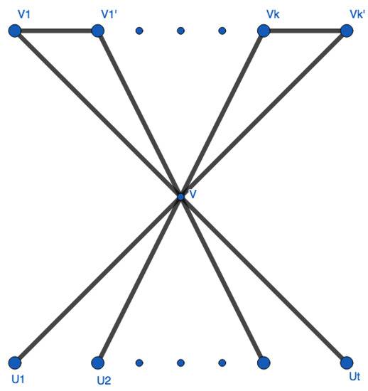
Figure 1. A tight example.

4. Remarks

As is known, fullerene graphs have regular structures with the degrees of all vertices equal to three (due to the typical tri-coordination of sp -hybridized carbon atoms) [a]. The possible application of the cactus graphs may deal with the carbon-based structures containing the carbon atoms with different coordination. In such structures, tetra-coordinated carbon atoms may correspond to the vertices common for simple cycles of cacti. In this aspect, cactus graphs seem applicable to the structure description of mixed carbon allotropes comprising a challenge for current carbon science [19,20,21].

References

- Nikiforov, V. Merging the A- and Q-spectral theories. Appl. Anal. Discret. Math. 2017, 11, 81–107. [Google Scholar] [CrossRef]
- Giannelli, E.; Law, S.; Martin, S. On the p′-Subgraph of the Young Graph. Algebras Represent. Theory 2018, 22, 627–650. [Google Scholar] [CrossRef]
- Ye, M.-L.; Fan, Y.-Z.; Wang, H.-F. Maximizing signless Laplacian or adjacency spectral radius of graphs subject to fixed connectivity. Linear Algebra Its Appl. 2010, 433, 1180–1186. [Google Scholar] [CrossRef]
- Li, S.; Zhang, M. On the signless Laplacian index of cacti with a given number of pendant vertices. Linear Algebra Its Appl. 2012, 436, 4400–4411. [Google Scholar] [CrossRef]
- Feng, L.; Li, Q.; Zhang, X.-D. Minimizing the Laplacian spectral radius of trees with given matching number. Linear Multilinear Algebra 2007, 55, 199–207. [Google Scholar] [CrossRef]
- Xing, R.; Zhou, B. On the least eigenvalue of cacti with pendant vertices. Linear Algebra Its Appl. 2013, 438, 2256–2273. [Google Scholar] [CrossRef]
- Yu, A.; Lu, M.; Tian, F. On the spectral radius of graphs. Linear Algebra Its Appl. 2004, 387, 41–49. [Google Scholar] [CrossRef]
- Chen, Y. Properties of spectra of graphs and line graphs. Appl. Math. J. Chin. Univ. Ser. B 2002, 17, 371–376. [Google Scholar]
- Lovász, L.; Pelikán, J. On the eigenvalues of trees. Period. Math. Hungar. 1973, 3, 175–182. [Google Scholar] [CrossRef]
- Cvetković, D.; Rowlinson, P.; Simić, S.K. Signless Laplacians of finite graphs. Linear Algebra Its Appl. 2007, 423, 155–171. [Google Scholar] [CrossRef]
- Zhou, B. Signless Laplacian spectral radius and Hamiltonicity. Linear Algebra Its Appl. 2010, 432, 566–570. [Google Scholar] [CrossRef]
- Lin, H.; Zhou, B. Graphs with at most one signless Laplacian eigenvalue exceeding three. Linear Multilinear Algebra 2015, 63, 377–383. [Google Scholar] [CrossRef]
- Nikiforov, V.; Pastén, G.; Rojo, O.; Soto, R.L. On the Aα-spectra of trees. Linear Algebra Its Appl. 2017, 520, 286–305. [Google Scholar] [CrossRef]
- Borovićanin, B.; Petrović, M. On the index of cactuses with n vertices. Publ. Inst. Math. 2006, 79, 13–18. [Google Scholar] [CrossRef]
- Chen, M.; Zhou, B. On the Signless Laplacian Spectral Radius of Cacti. Croat. Chem. Acta 2016, 89, 493–498. [Google Scholar] [CrossRef]
- Wu, J.; Deng, H.; Jiang, Q. On the spectral radius of cacti with k-pendant vertices. Linear Multilinear Algebra 2010, 58, 391–398. [Google Scholar] [CrossRef]
- Shen, Y.; You, L.; Zhang, M.; Li, S. On a conjecture for the signless Laplacian spectral radius of cacti with given matching number. Linear Multilinear Algebra 2017, 65, 457–474. [Google Scholar] [CrossRef]
- Xue, J.; Lin, H.; Liu, S.; Shu, J. On the Aα-spectral radius of a graph. Linear Algebra Its Appl. 2018, 550, 105–120. [Google Scholar] [CrossRef]
- Sabirov, D.S.; Ori, O.; László, I. Isomers of the C fullerene: A theoretical consideration within energetic, structural, and topological approaches. Fuller. Nanotub. Carbon Nanostruct. 2018, 26, 100–110. [Google Scholar] [CrossRef]
- Ruoff, R.S. A perspective on objectives for carbon science. Carbon 2018, 132, 802. [Google Scholar] [CrossRef]
- Bianco, A.; Chen, Y.; Chen, Y.; Ghoshal, D.; Hurt, R.H.; Kim, Y.A.; Koratkar, N.; Meunier, V.; Terrones, M. A carbon science perspective in 2018: Current achievements and future challenges. Carbon 2018, 132, 785–801. [Google Scholar] [CrossRef]
© 2020 by the authors. Licensee MDPI, Basel, Switzerland. This article is an open access article distributed under the terms and conditions of the Creative Commons Attribution (CC BY) license (http://creativecommons.org/licenses/by/4.0/).