Abstract
The stability problem of the stationary rotation of N identical point vortices is considered. The vortices are located on a circle of radius at the vertices of a regular N-gon outside a circle of radius R. The circulation around the circle is arbitrary. The problem has three parameters N, q, , where . This old problem of vortex dynamics is posed by Havelock (1931) and is a generalization of the Kelvin problem (1878) on the stability of a regular vortex polygon (Thomson N-gon) on the plane. In the case of , the problem has already been solved: in the linear setting by Havelock, and in the nonlinear setting in the series of our papers. The contribution of this work to the solution of the problem consists in the analysis of the case of non-zero circulation . The linearization matrix and the quadratic part of the Hamiltonian are studied for all possible parameter values. Conditions for orbital stability and instability in the nonlinear setting are found. The parameter areas are specified where linear stability occurs and nonlinear analysis is required. The nonlinear stability theory of equilibria of Hamiltonian systems in resonant cases is applied. Two resonances that lead to instability in the nonlinear setting are found and investigated, although stability occurs in the linear approximation. All the results obtained are consistent with those known for . This research is a necessary step in solving similar problems for the case of a moving circular cylinder, a model of vortices inside an annulus, and others.
MSC:
76B47; 34D20; 70K30
1. Introduction
The classical hydrodynamics of an ideal fluid uses a model of point vortices (or parallel vortex threads) that goes back to H. Helmholtz. Let’s list the reviews that contain various tasks that use this model [1,2,3,4,5,6,7]. G. Kirchhoff obtained the Hamiltonian form of the motion equations of point vortices on the plane and indicated possible first integrals. These integrals were sufficient for the complete integrability of the problem in the case of two and three vortices.
The point vortices model was used by Kelvin (1878) in the construction of his theory of the atom. Although this theory was rejected the mathematical model survived. Now it took on new urgency in connection with the theory of vortices in superfluid [8] and the electronic columns [9]. Kelvin posed the stability problem for the stationary rotation of the system of N equal vortices located in the vertices of regular N-gon (Thomson N-gon). A long history of research on this problem is described in [10], where a review of the experimental and theoretical work is given. The stability analysis in linear approximation was done by J. Thomson (1883) and T. Havelock (1931). Nonlinear stability analysis was performed much later [10].
From the general papers on the movement of point vortices in a fluid bounded by absolutely smooth walls, it should be noted the Lin’s paper [11], in which, in particular, it is shown that the motion equations of vortices inside and outside the circle are Hamiltonian. The model of vortices outside the circle takes into account that the circulation around the circle can be arbitrary one [11,12]. The case of is of particular interest because when the radius of the circle tends to zero, we come to the Kirchhoff’s model on the plane.
Havelock investigated the stability problem of a regular vortex polygon inside and outside the circle in the case of in a linear setting [13]. He obtained conditions under which the corresponding linearized system has exponentially growing solutions. Thus, after this paper, the question of stability in the case of remained open when all the eigenvalues of the linearization matrix are purely imaginary or null. Nonlinear analysis, in this case, is performed for the problem inside the circle in the papers [14,15] and for the problem outside the circle in the series of the papers [16,17,18,19]. The general theory of nonlinear stability analysis of solutions of Hamiltonian systems by methods of Kolmogorov–Arnold–Moser theory (KAM-theory) was used [20,21,22,23]. In particular, the quadratic part of the Hamiltonian was studied. Resonant cases requiring analysis of the third and fourth-order terms of the Taylor series expansion of the Hamiltonian were considered separately. It turned out that two of them lead to instability, although in the linear setting there is stability.
The purpose of this paper is to study the stability of a regular vortex N-gon in the case of an arbitrary circulation . The linearized system and the quadratic part of the Hamiltonian are investigated. This allowed us to divide the parameter space of the problem into three areas: the areas of orbital stability and instability in the nonlinear setting, and the area where linear stability takes place and nonlinear analysis is required.
In this paper, the stability theory of Hamiltonian systems in resonant cases has been used [23,24]. We applied it to study the influence of circulation on stability in two resonant cases, the instability of which was found at in [17,18]. These are critical case of the double-zero resonance at and the case of resonance at .
The model of point vortices outside the circular domain considered by us is a limiting case of more complex models, for example, the movement of discrete vortices in an annular, in a deformation flow [25], the model of moving cylinder interacting with the configuration of N point vortices [26]. Therefore, our research is a necessary step in the analysis of similar problems in all these models.
2. Problem Formulation
The motion of the system N identical point vortices of intensity outside the circle of radius R is described by the system (see, for example [12])
Here , are complex variables, , are Cartesian coordinates of kth vortex, is the reflection of the kth vortex from the boundary of the circle, parameter is circulation around circle.
Let us assume that
In the case, and the system of Equation (1) transforms to the Kirchhoff equations of motion of point vortices on the plane.
Thus, a system of N identical vortices located on a circle of radius at the vertices of a regular N-gon rotates with a constant angular velocity (see Figure 1).
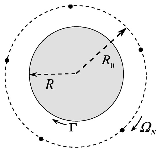
Figure 1.
Thomson vortex N-gon outside a circle.
The angular velocity decreases monotonously over at fixed values . The vortex N-gon changes the rotation direction at a fixed with the growth of parameter q on the curve
In the case, the rotation direction with the growth of q does not change. The graphs of are shown in Figure 2.
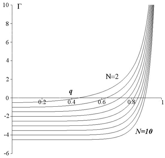
Figure 2.
The graphs of the curves in the interval such that the angular velocity . The graphs are shown from top to bottom in order of increasing .
The problem of stability of stationary rotation (4) is studied in the following sections.
3. Stability of a Regular Vortex -gon for
We consider the case when circulation around the boundary is zero: .
In this case, the stability problem of the stationary rotation of the Thomson vortex N-gon was solved in the linear setting by Havelock [13]. He found that the corresponding linearized system has exponentially growing solutions for , if the parameter is greater than the critical value : , and for the instability occurs for all .
In the papers [17,18] for odd and in [16] for even , it is shown with the help of analysis of the quadratic part of the Hamiltonian that for there is orbital stability in the exact nonlinear setting. In the case of even N the value . The critical values of and are shown in the Table 1.

Table 1.
The critical values and for in the case .
Nonlinear analysis was performed using KAM-theory methods (see, for example [23,24]). It was held at a point in the case of even [16] and on the segment for odd [17,18]. In particular, all resonances encountered in the problem were found and studied. It turned out that only two of them lead to instability. These are the resonance of the double zero at , if , and the resonance at in the point .
4. Linear Analysis of Stability of the Vortex -gon in the Case of Arbitrary
4.1. The Perturbations Equation
The change of variables
and scaling of time transforms the system (2) and (3) to the perturbations equations
with the Hamiltonian
The Taylor series expansion of the Hamiltonian in powers of in the neighborhood of the zero solution is
The terms of degree higher than three are omitted. The linear terms is zero: . The quadratic form can be represented as
where is the scalar product of two vectors.
The linearization matrix of the system (8) in the neighborhood of the zero solution has the form
The matrices are circulants of size , moreover are symmetric matrices, and is a skew-symmetric one. They are polynomials of the cyclic matrix (see, for example Appendix A of [10]):
where is unit matrix.
Only the coefficient depends on the parameter :
where
The coefficients , , , and , do not depend on , and therefore, they match the corresponding coefficients written out in the papers [13] for the case of :
The eigenvalues , and of matrices , and are calculated with the help of the formulas
The value has the form
where
The values and the eigenvalues , are the same as in the papers [13]:
The matrices , have the same eigenvectors
In the case of even , there is another eigenvector
For the matrices , and , the relations are performed:
The eigenvalues of matrix are the roots of the polynomials (see [14], Section 3.1 of [27]):
4.2. Orbital Stability and Instability of Two-Dimension Invariant Set: General Definitions and Theorems
The stationary rotation regime (4) is Lyapunov unstable for any . Indeed, the angular speed of rotation depends on the radius . Therefore, for an arbitrarily small perturbation of the radius , the perturbed Thomson N-gon will move away from the undisturbed one by an order of diameter . Thus, we need to clarify our definitions of stability and instability.
In this paper, as in [27], stability of a stationary solution (4) is understood as orbital stability or stability of the continuous family of equilibria
of the perturbations Equations (8) and (9).
The instability is instability of the invariant set of the system (8) and (9):
formed by all the orbits of a continuous family (4) depending on the parameter (For more information, see Section 3 of [27]).
The matrices and have the same structure as in [27]. Therefore, repeating verbatim the arguments about the orbital stability of the equilibrium family and the instability of the invariant set , given in Sections 3.2 and 3.3 of [27], we obtain the following statements.
Proposition 1
(Section 3.2 of [27]). Let roots of the polynomials , and the value , given by Formulas (23) and (18)–(20), have identical sign. Then,
Proposition 2
(Section 3.3 of [27]). Let the inequality
be satisfied for at least one . The values and are given by Formulas (18)–(20).
Then the linearization matrix has at least one eigenvalue (24) with a positive real part and the invariant set is unstable.
Proposition 3
(Section 3.3 of [27]). Let inequalities
are valid for all , then all eigenvalues of the matrix lie on the imaginary axis, and stability by linear approximation takes place.
If, in addition, the conditions of Proposition 1 are violated, then the linear approximation is not enough to analyze the stability.
According to the properties and of the Proposition A1 of Appendix A, the value is positive for any N and :
and the value
Taking into account these inequalities, we reformulate the Propositions 1–3 as follows.
Theorem 1.
The stationary rotation (4) of the Thomson vortex N-gon is
- 1°
- orbitally stable in an exact nonlinear setting if the inequalitiesare valid;
- 2°
- unstable if there is at least one value such that
- 3°
- If conditions and are not valid, then the solution (4) is stable in a linear setting, and nonlinear analysis is required to solve the stability problem.
4.3. Stability Diagram of a Regular Vortex N-gon
Let’s introduce the following notation
It is numerically established at that the following conditions
are valid.
Conditions (33) and (34) have been checked for a number of values and no violations of them have been found anywhere. It is possible that these conditions are also true for arbitrary N.
In similar stability problems for other models of vortex dynamics the conditions (29), (33) and (34) may not be valid, for example, for a two-fluid plasma model [28].
Let the values and be given by the formulas:
If the relations (33) and (34) are fulfilled, then the condition (31) is
and the condition (32) has the form
Applying the Theorem 1 leads to results on the stability of stationary rotation of a Thomson vortex N-gon, schematically shown in Figure 3. The curves and divide the parameter space of the problem into the areas with different types of stability. Gray color indicates the area where condition of the Theorem 1 is valid, the vertical shading is area, where the condition is valid, and white color is one, where both conditions and are not valid.
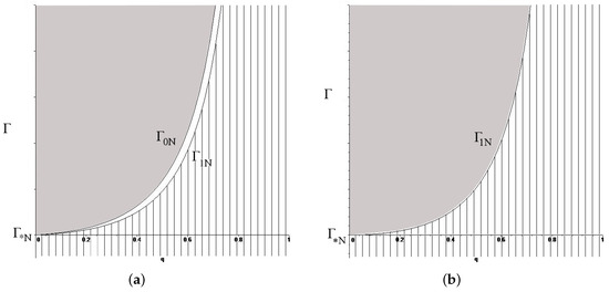
Figure 3.
Schematic stability diagram of the Thomson vortex N-gon: (a) The case of odd ; (b) The case of even . Gray is the area of orbital stability in an exact nonlinear setting, the vertical shading is the area of instability, white color and neutral curves , are the area of linear stability, where is required nonlinear analysis. The diagram is true for and for if the conditions (33) and (34) are valid.
The value is
The values of for are shown in the Table 2. For the values .
Table 2.
The critical values of for .
In the case of odd , a linear stability domain, which requires nonlinear analysis, exists for all , since according to the property of the Proposition A1, the inequality is valid.
Note that instability occurs for all values of , if . If , all three areas always exist. In the case of even N, the domain, where nonlinear analysis is required, consists only of a curve . If , the stability interval exists only for [13]. In the case the linear stability domain consists of one point , that corresponds the problem of stability of a Thomson heptagon on a plane [10].
According to the general theory (see, for example [23,24]) in the white domain in the Figure 3 and in the neutral curves and instability is possible when the eigenvalues of the linearization matrix (12) are in resonant relations. Nonlinear terms of the Taylor series of the Hamiltonian (9), starting from the third degree, must satisfy some additional conditions. In [17,18] for in the segment two resonances leading to instability were found in the case : in the point in the case and in the point in the case . These are the double-zero resonance (diagonalizable case) and the 1:2 resonance, respectively. In the following sections, they are studied for arbitrary values .
5. The Double-Zero Resonance in the Stability Problem of the Thomson Vortex Triangle
Let and a point lies on the resonance curve given by Equation (35). There is a four-fold zero eigenvalue among the eigenvalues (24) of the linearization matrix . In addition to , two other null eigenvalues appear: and . In this section, it will be shown that in this case the invariant set given by the Formula (26) is unstable. To prove it, we construct a reduced system following the paper [17].
We introduce the change of variables [17,23]
where is a symplectic matrix [29]:
or
Here, is k-th column of matrix , , are basis vectors defined by equalities (21) for :
is zero vector, According to the Formula (35) and the Proposition A1, values and are positive since .
In new variables the Hamiltonian given by the Formula (9) has a cyclic variable , since the Hamiltonian (9) is invariant with respect to change of variables , , which in the vector form is written as
The vectors and are the eigenvector and adjoined vector of a linearization matrix . They correspond to the double zero eigenvalue :
The cyclic variable and the variable correspond to the vectors and , respectively.
Methods for investigating equilibrium stability for systems with cyclic variables were developed by Routh [30]. Assuming , we obtain a reduced system with the reduced Hamiltonian
The invariant set is the subspace formed by the vectors and . A reduced system with the Hamiltonian (43) is defined in a subspace orthogonal to the invariant set . Hence, the instability of the zero equilibrium of a reduced system is the instability of the invariant set (26).
The Taylor series expansion of Hamiltonian (43) in the resonant curve has the form
The terms of degree higher than three are omitted.
According to [31], the zero equilibrium is unstable if and the third-degree form is different from the identity zero on the set of zeros of the quadratic part .
In the Figure 4 it is shown that coefficient is positive for all . The quadratic form vanishes on the set
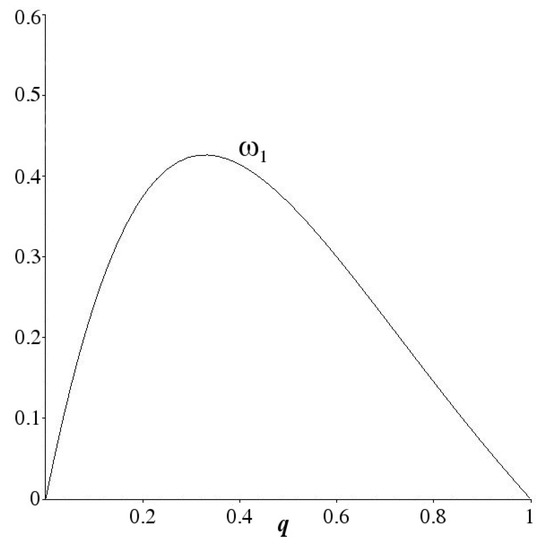
Figure 4.
The graph of the coefficient given by equality (45) in the interval .
The calculations showed that the third-degree form on this set has the form
As you can see from Figure 5 the coefficient is not zero.
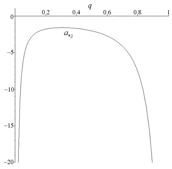
Figure 5.
The graph of the coefficient given by Formula (46) in the interval .
Thus, the stationary rotation (4) of the Thomson vortex triangle is unstable at all points of the resonance curve at the interval .
The function turns to zero at the point , that is consistent with the result of [17].
6. The Resonance 1:2 in the Stability Problem of the Thomson Vortex Pentagon
Let and the condition
is valid. Here functions and are given by Formula (35). Then the points lie in the white domain in the Figure 3, where linear stability takes place and the stability problem requires nonlinear analysis.
Following the paper [18], we introduce change of variables
where is symplectic matrix
Here , are basis vectors given by equalities (21) for , is zero vector,
In the considered condition (47) the statement of the Theorem 1 is performed and the inequality is valid for any .
In the new variables , the Hamiltonian defined by Formula (9) has cyclic variable . Assuming , we obtain reduced system.
We introduce the complex variables :
and obtain reduced system with the Hamiltonian W. The calculations showed that the Taylor series expansion of this Hamiltonian in a neighborhood of the zero equilibrium has the form
The terms of the third degree and higher except for the written one are omitted. The quadratic part of Hamiltonian W has a normal form:
Values are calculated with the help of the formulas
where defined by equality (24).
According to the paper [18] in the case the resonance leads to instability for .
We study the resonance
in the case of the arbitrary . The Equation (54) gives the curve where the resonance 1:2 occurs:
Here the values , and are given by Formulas (19) and (20). The curve is defined on the interval , . Its schematic image is shown in the Figure 6. The graphs of coefficient are shown in Figure 7 for .
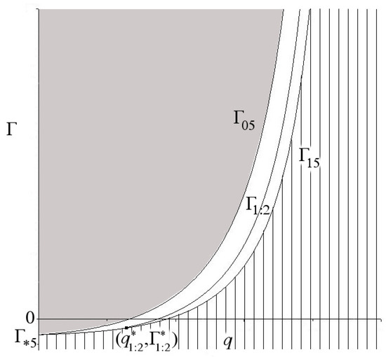
Figure 6.
Schematic stability diagram of the Thomson vortex pentagon. Grey color is the domain of orbital stability in an exact nonlinear setting, the vertical shading and the curve are instability domain, white color and neutral curves , are linear stability domains, which need nonlinear analysis.
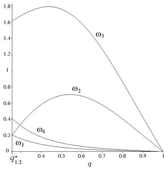
Figure 7.
The graphs of coefficients , on the resonance curve for , .
According to [23,32], in the absence of other resonances of the form
the zero equlibrium of the system with Hamiltonian (51)–(54) is unstable, if the inequality
is valid, that is shown in the Figure 8.
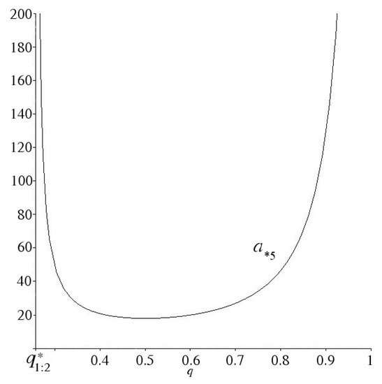
Figure 8.
The resonance 1:2. The graph of coefficient in the interval .
As seen in Figure 7, in addition to the equality (54) on the curve , other resonant relations of the form (56) take place only at two points. The equality is performed at the point , , and the equality is valid at the point . Here , . The stability problem at these points requires additional nonlinear analysis.
Thus, the invariant set is unstable on the curve when and . The domain and does not contain the points of resonance 1:2 ().
7. Conclusions
This paper is a natural continuation of the series of articles [13,16,17,18,19]. The novelty of the result is that the stability problem of the Thomson vortex N-gon outside circular domain is considered in the case of an arbitrary circulation around the boundary. Previously in the papers [13,16,17,18,19] it was assumed that .
The stability analysis was based on the Routh theory for the study of Hamiltonian systems with cyclic variables [30] and on a generalization of the approach developed in Section 3 of [27] for the study of a Thomson vortex N-gon in the case of an arbitrary Hamiltonian that depends only on the distances between point vortices.
The results of the study of the linearization matrix and the quadratic part of the Hamiltonian are presented as stability diagrams in Figure 3 if the conditions (33) and (34) are valid. For and in some cases , we checked their execution numerically. For a nonlinear stability analysis has been performed in the critical case of two-fold zero on the corresponding resonant curve , . It is shown that the stationary rotation of the vortex triangle is unstable. For a vortex pentagon , a nonlinear analysis has been performed in the critical case of the resonance 1:2 on the curve , , shown schematically in Figure 6. Instability has been proved. The resonance curves and intersect in the point . There are no points of resonance 1:2 in domain and , although it requires nonlinear analysis.
Possible directions of development of this paper are related to the nonlinear analysis of the stability problem in the white domain in Figure 3 at and on its boundaries. To do this, we need to apply the KAM-theory methods (see, for example [23]), in particular, list and study all resonances encountered in this problem. Among them we will consider the points found in the Section 6. These are the point where two resonances and intersect, and the point , where the resonances are and .
The method of nonlinear analysis was previously tested for a model of vortices inside a circular domain in [14,15] and outside the circle in the case of zero circulation in [16,17,18,19].
Of particular interest is the study of the boundary of the instability domain. The answer to this question is important in order to find out what this border is: “dangerous” or “safe” according to Bautin [24,33]? In other words, there is a hard or soft loss of stability of the Thomson polygon when the parameter q increases and passes through the critical value at a fixed ?
The results of the study can also be generalized to the case of a moving cylinder interacting with the configuration of N point vortices [26], the model of Thomson N-gon in two-layer fluid [27,34] and others.
Author Contributions
Conceptualization, L.K. and I.O.; funding acquisition, L.K. and I.O; investigation, L.K. and I.O; methodology, L.K. and I.O; writing, original draft, L.K. and I.O; writing, review and editing, L.K. and I.O. All authors have read and agreed to the published version of the manuscript.
Funding
The research was funded by Russian Foundation for Basic Research (Projects No. 20-55-10001).
Conflicts of Interest
The authors declare no conflict of interest.
Appendix A. Properties of Eigenvalues λ1k, λ2k and iλ0k of Matrices F1, F2 and G0
The following proposition sets the properties of quantities , and given by equalities (18)–(20).
Proposition A1.
The following statements are valid.
- The function is positive in the interval :
- The function does not have zeros in the interval :
- The function given by Formula (19) satisfies inequalityin the interval .
- In the case the value is positive:is defined by Formula (35).
- In the case of odd for any the inequalityis valid.
Proof.
From the equalities (18)–(20), it follows that
Thus, it is sufficient to consider the cases .
To prove the statement , we write the value as
where
According to Descartes’ rule of signs [35], the number of positive roots of the polynomial is at most the number of sign changes in the sequence of its coefficients, and that the difference between these two numbers is always even. Zero coefficients are not taken into account when calculating sign changes.
The series of the polynomial coefficients has four sign changes, and the polynomial has a four-fold root . Indeed, the polynomial and its first three derivatives , are
They vanish in the point . The four derivative at this point is different from zero:
Therefore, the polynomial does not have roots in the interval . Since the value , then for all . The statement is proved.
Similarly, the statement is proved. The function is rewritten as
where
The series of the polynomial coefficients has three sign changes, and the polynomial itself has a three-fold root . According to Descartes’ rule of signs, there are no other positive roots of the polynomial and, accordingly, the function .
To prove the inequality (A3) in the statement , we present the difference as:
The polynomial has double root and two sign changes in the series of coefficients. Therefore, there are no other positive roots. Since the value is positive, the inequalities and (A3) are valid for all and any N.
The property follows from the statement and the equality (35). In the case of we have:
The validity of the property follows from the equality (35) and the statements and . Indeed, for
The Proposition A1 is proved. □
References
- Aref, H. Point vortex dynamics: A classical mathematics playground. J. Math. Phys. 2007, 48, 065401. [Google Scholar] [CrossRef]
- Aref, H.; Newton, P.K.; Stremler, M.A.; Tokieda, T.; Vainchtein, D.L. Vortex Crystals. Adv. Appl. Mech. 2003, 39, 1–79. [Google Scholar]
- Newton, P.K. The n-Vortex Problem: Analytical Techniques; Appl. Math. Sci.; Springer: New York, NY, USA, 2001; Volume 145. [Google Scholar]
- Borisov, A.V.; Mamaev, I.S. Mathematical Methods in the Dynamics of Vortex Structures; Institute of Computer Sciences: Moscow/Izhevsk, Russia, 2005. [Google Scholar]
- Kilin, A.A.; Borisov, A.V.; Mamaev, I.S. Dynamics of point vortices inside and outside of a circular domain. In Fundamental and Applied Problems in Vortex Theory; Institute of Computer Sciences: Moscow/Izhevsk, Russia, 2003; pp. 414–440. [Google Scholar]
- Saffman, P.G. Vortex Dynamics; Series Cambridge Monogr. Mech. and Appl. Math. Cambridge University Press: Cambridge, UK, 1992. [Google Scholar]
- Kozlov, V.V. General Theory of Vortices; Dynamical systems X., Encyclopaedia Math. Sci., 67; Springer: Berlin, Germany, 2003. [Google Scholar]
- Yarmchuk, E.; Gordon, M.; Packard, R. Observation of stationary vortex array in rotating superfluid helium. Phys. Rev. Lett. 1979, 43, 214–217. [Google Scholar] [CrossRef]
- Fine, K.; Cass, A.; Flynn, W.; Dryscoll, C. Relaxation of 2D Turbulence to Vortex Crystal. Phys. Rev. Lett. 1995, 75, 3277–3280. [Google Scholar] [CrossRef] [PubMed]
- Kurakin, L.G.; Yudovich, V.I. The stability of stationary rotation of a regular vortex polygon. Chaos 2002, 12, 574–595. [Google Scholar] [CrossRef] [PubMed]
- Lin, C.C. On the motion of vortices in two dimensions. I, II. Proc. Natl. Acad. Sci. USA 1941, 27, 575–577. [Google Scholar] [CrossRef]
- Milne-Thomson, L.M. Theoretical Hydrodynamics; Macmillan: London, UK, 1968. [Google Scholar]
- Havelock, T.H. The stability of motion of rectilinear vortices in ring formation. Lond. Edinb. Dublin Philos. Mag. J. Sci. 1931, 11, 617–633. [Google Scholar] [CrossRef]
- Kurakin, L.G. Stability, resonances, and instability of the regular vortex polygons in the circular domain. Dokl. Phys. 2004, 49, 658–661. [Google Scholar] [CrossRef]
- Kurakin, L.G. On the Stability of Thomson’s Vortex Pentagon Inside a Circular Domain. Regul. Chaotic Dyn. 2012, 17, 150–169. [Google Scholar] [CrossRef]
- Kurakin, L.G.; Ostrovskaya, I.V. Stability of the Thomson Vortex Polygon with Evenly Many Vortices outside a Circular Domain. Sib. Math. J. 2010, 51, 463–474. [Google Scholar] [CrossRef]
- Kurakin, L.G. The stability of the steady rotation of a system of three equidistant vortices outside a circle. J. Appl. Math. Mech. 2011, 75, 227–234. [Google Scholar] [CrossRef]
- Kurakin, L.G.; Ostrovskaya, I.V. Nonlinear stability analysis of a regular vortex pentagon outside a circle. Regul. Chaotic Dyn. 2012, 17, 385–396. [Google Scholar] [CrossRef]
- Kurakin, L.G.; Melekhov, A.P.; Ostrovskaya, I.V. A survey of the stability criteria of Thomson’s vortex polygons outside a circular domain. Bol. Soc. Mat. Mex. 2016, 22, 733–744. [Google Scholar] [CrossRef]
- Kolmogorov, A.N. On conservation of conditionally periodic motions for a small change in hamilton’s function. Dokl. Akad. Nauk SSSR 1954, 98, 527–530. [Google Scholar]
- Arnold, V.I. Small denominators and problems of stability of motion in classical and celestial mechanics. Russ. Math. Surv. 1963, 18, 85–191. [Google Scholar] [CrossRef]
- Moser, J. Lectures on Hamiltonian Systems; Memoirs of the American Mathematical Society: Providence, RI, USA, 1968; Volume 81. [Google Scholar]
- Markeev, A.P. Libration Points in Celestial Mechanics and Space Dynamics; Nauka: Moscow, Russia, 1978. [Google Scholar]
- Khazin, L.G.; Shnol, E.E. Stability of Critical Equilibrium States; Manchester University Press: Manchester, NH, USA, 1991. [Google Scholar]
- Koshel, K.V.; Ryzhov, E.A.; Carton, X.J. Vortex Interactions Subjected to Deformation Flows: A Review. Fluids 2019, 4, 14. [Google Scholar] [CrossRef]
- Borisov, A.V.; Mamaev, I.S.; Romodanov, S.M. Dynamic interaction of point vortices and a two-dimentional cylinder. J. Math. Phys. 2007, 48, 065403. [Google Scholar] [CrossRef]
- Kurakin, L.G.; Lysenko, I.A.; Ostrovskaya, I.V.; Sokolovskiy, M.A. On stability of the Thomson’s vortex n-gon in the geostrophic model of the point vortices in two-layer fluid. J. Nonlinear Sci. 2019, 29, 1659–1700. [Google Scholar] [CrossRef]
- Kurakin, L.G.; Lysenko, I.A. On the stability of the orbit and the invariant set of Thomson’s vortex polygon in a two-fluid plasma. Rus. J. Nonlin. Dyn. 2020, 16, 3–11. [Google Scholar]
- Gantmacher, F.R. Lectures on Analytical Mechanics; Glavnaya Redaktsiya Fiziko-Matematicheskoj Literatury, Nauka: Moscow, Russia, 1966. [Google Scholar]
- Routh, E.J. A Treatise on the Stability of a Given State Motion; Macmillan: London, UK, 1877; 108p. [Google Scholar]
- Sokol’sky, A.G. On Stability of an Autonomous Hamiltonian System with Two Degrees of Freedom under First-Order Resonance. J. Appl. Math. Mech. 1977, 41, 20–28. [Google Scholar] [CrossRef]
- Markeev, A.P. Stability of a canonical system with two degrees of freedom in the presence of resonance. J. Appl. Math. Mech. 1968, 32, 766–772. [Google Scholar] [CrossRef]
- Bautin, N.N. Behavior of Dynamics Systems Near the Boundary of the Stability Region; Gostekhizdat: Moscow, Russia, 1984. [Google Scholar]
- Kurakin, L.G.; Ostrovskaya, I.V.; Sokolovskiy, M.A. On the stability of discrete tripole, quadrupole, Thomson’ vortex triangle and square in a two-layer/homogeneous rotating fluid. Regul. Chaotic Dyn. 2016, 21, 291–334. [Google Scholar] [CrossRef]
- Kurosh, A.G. Course of Higher Algebra; Nauka: Moscow, Russia, 1962. [Google Scholar]
© 2020 by the authors. Licensee MDPI, Basel, Switzerland. This article is an open access article distributed under the terms and conditions of the Creative Commons Attribution (CC BY) license (http://creativecommons.org/licenses/by/4.0/).