Implicit-Explicit Methods for a Convection-Diffusion-Reaction Model of the Propagation of Forest Fires

Abstract

Numerical techniques for approximate solution of a system of reaction-diffusion-convection partial differential equations modeling the evolution of temperature and fuel density in a wildfire are proposed. These schemes combine linearly implicit-explicit Runge–Kutta (IMEX-RK) methods and Strang-type splitting technique to adequately handle the non-linear parabolic term and the stiffness in the reactive part. Weighted essentially non-oscillatory (WENO) reconstructions are applied to the discretization of the nonlinear convection term. Examples are focused on the applicative problem of determining the width of a firebreak to prevent the propagation of forest fires. Results illustrate that the model and numerical scheme provide an effective tool for defining that width and the parameters for control strategies of wildland fires.

1. Introduction

1.1. Scope

It is the purpose of this contribution to provide an efficient numerical method for the solution of a wildland fire model [1]. This model can be expressed as a convection-diffusion-reaction system of the type

$$\begin{array}{cc}\hfill \frac{\partial u}{\partial t}+\mathit{w}(\mathit{x},t)·\nabla u& =\nabla ·\left(K\left(u\right)\nabla u\right)+f(u,v,\mathit{x}),\frac{\partial v}{\partial t}=g(u,v),\hfill \end{array}$$

(1)

where t is time, $\mathit{x}\in \mathsf{\Omega }$ is the spatial variable where $\mathsf{\Omega }\subset {\mathbb{R}}^2$, and $u=u(\mathit{x},t)$ and $v=v(\mathit{x},t)$ are the sought scalar functions. Here u represents the non-dimensionalized temperature and v the non-dimensionalized mass fraction of solid fuel. Moreover, K is a given diffusion coefficient that depends only on u, and $\mathit{w}$ is an advection velocity that represents wind speed. It is assumed that $\mathrm{div}\mathit{w}=0$. The functions $f(u,v,\mathit{x})$ and $g(u,v)$ are the reactive part of the model. (These ingredients will be specified further below.) The evolution of a wildfire is described by the system (1) together with zero-flux boundary conditions

$$\left(u\mathit{w}-K\left(u\right)\nabla u\right)·\mathit{n}=0,(\mathit{x},t)\in \partial \mathsf{\Omega }\times (0,+\infty ),$$

(2)

where $\mathit{n}$ is the unit normal vector to $\partial \mathsf{\Omega }$, and the initial conditions

$$u(\mathit{x},0)=u_0\left(\mathit{x}\right),v(\mathit{x},0)=v_0\left(\mathit{x}\right),\mathit{x}\in \mathsf{\Omega }.$$

(3)

Explicit numerical schemes for (1) on a uniform Cartesian grid of meshwidth $\Delta x$ and time step $\Delta t$ are easy to implement but are associated with a Courant–Friedrichs–Lewy (CFL) stability condition [2] that imposes the proportionality $\Delta t\approx \Delta x^2$ [3,4,5,6,7,8,9,10,11,12,13]. This restriction makes long-term simulations of (1)–(3) on a uniform grid unacceptably slow. A well-known remedy consists in handling the diffusive term in (1) by an implicit discretization. The resulting semi-implicit or implicit-explicit (IMEX) schemes (e.g., [3,11]) are associated with an acceptable CFL condition $\Delta t\approx \Delta x$. (Here we recall that semi-implicit (or semi-explicit) and IMEX schemes are not the same; the former class usually comprises one-step schemes such as the implicit Euler scheme or the trapezoidal rule while the latter larger class is based on intertwined computations of the stages of explicit and implicit Runge–Kutta schemes.) However, the case that K depends nonlinearly on u needs to be handled by special nonlinear solvers [11] or by solving linear problems in each time step. These linear problems arise from carefully distinguishing between stiff and nonstiff unknowns in the discretized version of $\nabla ·\left(K\left(u\right)\nabla u\right)$ [3]. These variants will be addressed as nonlinearly implicit (NI-IMEX) and linearly implicit (LI-IMEX) schemes, respectively. In this work we focus on the implementation of LI-IMEX schemes.

On the other hand, the reaction term for this model imposes a very severe restriction on the global time step $\Delta t$. As a strategy to avoid this restriction, we propose a variant of the LI-IMEX scheme consisting in a Strang-type splitting technique. This technique consists in solving the convection-diffusion system for u and coupling this result with the solution of the ordinary differential equation (ODE) for u and v defined by the reaction terms (in which the convective and diffusive term is absent). This results in a numerical scheme that allows a less restrictive time step $\Delta t$.

The main research question of this paper is whether LI-IMEX schemes, possibly equipped with Strang-type operator splitting, indeed provide a gain in CPU time, and hence in efficiency if applied to the wildland fire model (1) under realistic choices of model functions and parameters. Here a gain is understood in comparison with the performance of explicit schemes. The result is not obvious, since LI-IMEX schemes permit larger time steps but are associated with additional computational effort related to the solution of linear systems in each iteration. A secondary research question consists in assessing the suitability of model (1) for the simulation of wildfire control strategies.

From a practical point of view, we address the importance of being able to simulate the effects of artificial firebreaks as a measure of prevention and control of forest fires. The effectiveness of a firebreak, which is normally created by cutting a lane into a forest, is strongly determined by its width, as is discussed in [14,15]. This motivates the implementation of scenarios, such as those shown here, in order to help solve the problem of determining an adequate width and thus protect a certain area from forest fire.

1.2. Related Work

The literature includes many approaches to studying forest fires such as physical models, cellular automata and artificial intelligence, to name a few. A general survey on the principles of mathematical modeling of forest fires is provided by Pastor et al. [16] and more recently by Eberle et al. [17]. Most continuous-in-space approaches to model and study forest fires lead to partial differential equations (PDEs) as local forms of the balance equations that describe fuel consumption and heat transfer. A discussion of recent developments of PDE-based forest fire models, as opposed to those based on cellular automata, is included in [18]. We herein directly use the two-PDE model formulated by Asensio and Ferragut [1]. This model is widely accepted and has laid the foundation for various developments such as the inclusion of vegetation, moisture and endothermic pyrolysis by means of a multivalued function representing the enthalpy [19,20]. Reports on implementation of the model by Asensio and Ferragut [1] within software packages for real scenarios include [17,21,22]. For sake of completeness, we mention that PDE-based models have also been developed for a refined description of the combustion front of a wildfire; see e.g., [23] and the references cited in that work.

Solutions to the model (1) may be obtained through numerical methods such as mixed finite elements, finite differences, or finite volumes. Due to the structure of Equation (1), there is ample theoretical support for a spatial semi-discretization of the model following a method-of-lines strategy. The resulting scheme turns out to be explicit due to the choice of ODE integrators. However, explicit schemes applied to reaction-diffusion problems strongly restrict the time step due to stability conditions. Therefore, our goal is to treat reaction and diffusion implicitly and convection explicitly. To avoid the need to solve nonlinear systems that appear in the implicit treatment of nonlinear diffusion, we propose LIMEX Runge–Kutta schemes introduced in [3,4].

To underline the relevance and novelty of implicit-explicit discretizations for the wildfire model (1), let us briefly review state-of-the-art methods used in some of the references. Asensio and Ferragut [1] employ mixed finite element methods for the spatial discretization combined with the Euler method in time, which leads to a semi-implicit scheme. The versions of this model with moisture and pyrolisis effects (involving enthalpy) that include heat either a non-local [19] or or a local (diffusive) model of heat radiation [20] are based on related semi-implicit [19] or implicit [20] time discretizations, based on explicit or implicit Euler time stepping. A broader discussion of numerical methods for wildfire models, some of them based on work not cited in this paper, is provided by Eberle et al. [17]. Their approach to discretize the model (4), (5) is based on a collocational method (using radial basis functions) for space discretization in combination with a Crank–Nicolson scheme for time stepping, including a stabilization of convective terms. This approach does not involve a weak formulation of the problem [17] (p. 1363). On the other hand, San Martin and Torres [22] devise a spectral differentiation method based on a method-of-lines formulation (discrete in space, continuous in time) for a version of the model (4), (5) with linear diffusion. This method is a formalism of expressing the spatial partial derivatives in terms of Fourier transforms of the unknowns (temperature and fuel). The time integration is done by the classical, explicit fourth-order Runge–Kutta method. Finally, we mention that the treatments by Barovik and Taranchuk [23] and Taranchuk and Barovik [24] employ finite difference methods with explicit Euler time stepping. All these approaches refer to different models but involve at least two unknowns, temperature and fuel. The discretization methods have in common, however, that the numerical solution is evolved over one single time step by discretizing each model ingredient either explicitly or implicitly. For all these approaches a more efficient alternative may arise through the intertwined explicit and implicit evaluations of stages of IMEX schemes, as is explained in Section 1.1. That said, improvements are most likely to accrue for base methods that are fully explicit, such as the one utilized in [23,24].

References to the various applications of IMEX methods for convection-diffusion-reaction problems, convection problems with stiff reaction terms, hyperbolic systems with relaxation and semi-discrete PDE solutions include [3,4,5,6,11,13,25].

1.3. Outline of the Paper

The remainder of the paper is organized as follows. In Section 2 the governing mathematical model is introduced. To this end, we formulate in Section 2.2 a model system of PDEs which that describes in simplified form the spatio-temporal evolution of temperature and fuel density. Section 3 is devoted to the description of the numerical schemes proposed to solve the PDE model. Values of the model parameters and an estimate of the maximum temperature attainable are provided in Section 2.4. Section 3.1 introduces the notation for two numerical schemes and details the discretization of the convective flux by a fifth-order weighted essentially non-oscillatory (WENO) reconstruction. In Section 3.2 the linearly implicit IMEX-RK method and in Section 3.3 the linearly implicit method IMEX-RK with Strang-type splitting are outlined. Section 4 is devoted to the presentation of numerical results. The examples correspond to four different scenarios. The first shows the numerical solution of the model considering an initial ignition in a domain with a constant fuel density. Results of this example, which also include a study of approximate $L^1$ errors, are shown in Section 4.1. In the second case we also impose an initial ignition but now with a terrain separated into two parts with different initial values for the fuel density. In the third we assume that the two regions that differ in the initial value for the fuel density are separated by a firebreak. In the fourth and last case we show the evolution of the variables in a terrain with random fuel density where the wind slightly changes its direction. The corresponding numerical examples are presented in Section 4.2, Section 4.3 and Section 4.4, respectively. Conclusions are collected in Section 5.

2. Mathematical Model

2.1. Model Development

The mathematical model follows the presentation by Asensio and Ferragut [1]. In a simplified setting, we consider the amount of solid fuel, but not its composition. The chemical reaction of fuel and oxidants into products is supposed to take place at the rate r defined by the Arrhenius equation

$$\begin{array}{c}\hfill r=Aexp\left(-\frac{E_{\mathrm{A}}}{RU}\right),\end{array}$$

where $E_{\mathrm{A}}$ denotes the activation energy, U is absolute temperature, $R=1.987207\mathrm{cal}/\left(\mathrm{K}\mathrm{mol}\right)$ is the universal gas constant, and A is a constant. A typical value is $E_{\mathrm{A}}\approx 20\mathrm{kcal}/\mathrm{mol}$ [26]. Furthermore, if Y denotes the mass fraction of fuel, then the rate of fuel consumption $S_{\mathrm{f}}$ can be chosen as $S_{\mathrm{f}}=-r\rho Y$, where $\rho$ is the density. The balance equation for the oxidant need not be considered [1]. Presupposing that the fire source is large (as should be typical for a wildfire), we may assume that the dominant mode of heat transfer is radiation. Heat flux transfer by radiation through a fuel bed can be derived from the Stefan–Boltzmann law (see [1,17] for details), which leads to the equation $q=-4\sigma \delta U^3\nabla U$ for the radiative heat flux, where $\sigma$ is the Stefan–Boltzmann constant and $\delta =\parallel \delta \parallel$ is the length of the optical path for radiation through the substance. Furthermore, we take into account vertical heat loss due to gravity by a natural convection term within the energy conservation equation, namely $h\left(\mathit{x}\right)(U-U_{\infty })$. Here h is the natural convection coefficient and $U_{\infty }$ stands for the ambient temperature. While $h=h\left(\mathit{x}\right)$ usually represents information on the local topography, we here consider h to be constant. On the other hand, we describe convection of heat due to wind by a term $\rho C\mathit{w}(\mathit{x},t)$. Here $\rho$ and C are the density and specific heat. The vector field $\mathit{w}=\mathit{w}(\mathit{x},t)$ is the wind velocity vector. We assume that temperature and velocity correspond to averaged values in a turbulent regime but that the reactive term is governed by the laminar regime. Under the latter assumption and denoting by H the heat of combustion, we may model the energy released in an exothermic reaction by

$$\begin{array}{c}\hfill Q=H{S}_{\mathrm{f}}=-HAexp\left(-\frac{E_{\mathrm{A}}}{RU}\right)\rho Y.\end{array}$$

Finally, we need to describe the change between the endothermic (solid) and the exothermic (gaseous) phase. This is done by the function

$$\begin{array}{c}\hfill s\left(U\right):=\left\{\begin{array}{cc}1\hfill & \mathrm{if}U\ge U_{\mathrm{pc}},\hfill \\ 0\hfill & \mathrm{if}U<U_{\mathrm{pc}}\hfill \end{array}\right.\end{array}$$

that describes phase change, which is supposed to occur at a temperature $U_{\mathrm{pc}}$. Utilizing this function allows us to handle both phases within the same system of equations. The basic processes that are described in this way are fuel combustion and heat generation when U exceeds the phase change temperature $U_{\mathrm{pc}}$.

2.2. Simplified Model in Final Form

Combining the previous ingredients, we obtain the following model:

$$\begin{array}{cc}\hfill \rho C\left({\displaystyle \frac{\partial U}{\partial t}}+\mathit{w}·\nabla U\right)-\nabla ·\left((4\sigma \delta U^3+k)\nabla U\right)& =s\left(U\right)HAexp\left(-\frac{E_{\mathrm{A}}}{RU}\right)\rho Y-h\left(\mathit{x}\right)(U-U_{\infty }),\hfill \end{array}$$

(4)

$$\begin{array}{cc}\hfill Y_t& =-s\left(U\right)YAexp\left(-\frac{E_{\mathrm{A}}}{RU}\right).\hfill \end{array}$$

(5)

We study the model (4), (5) on a two-dimensional domain $\mathsf{\Omega }\subset {\mathbb{R}}^2$ with a piecewise smooth boundary $\mathsf{\Gamma }=\partial \mathsf{\Omega }$. It is assumed that $\mathsf{\Omega }$ is large enough so that U and Y do not change on $\mathsf{\Gamma }$ during the simulation time $(0,t_{max})$. We may therefore impose either zero-flux or Dirichlet boundary conditions. Spatial heterogeneity can be represented by the functions $h=h\left(\mathit{x}\right)$ and the initial distribution of available fuel $Y_0=Y_0\left(\mathit{x}\right)$.

It is assumed that the thermal conductivity coefficient k is a positive constant. Thus, (4) is a nonlinear but strictly parabolic PDE whose solutions are smooth. This means that solutions of (4), (5) do not develop discontinuities (shocks).

2.3. Dimensionless Variables

The combustion model (4), (5) can be non-dimensionalized in a rational manner in order to elucidate the significant parameters. We use the Frank–Kamenetskii change of variables (see [26]). We fix a reference value for the temperature and the fuel in which an equilibrium can be assumed, namely the ambient temperature $U_{\mathrm{ref}}=U_{\infty }$ and the initial fuel. Since $Y_0$ may be variable, we set

$$\begin{array}{c}\hfill Y_{\mathrm{ref}}:=\frac{1}{\left|\mathsf{\Omega }\right|}{\int }_{\mathsf{\Omega }}{Y}_0\left(\mathit{x}\right)\mathrm{d}\mathit{x};\end{array}$$

likewise, we define

$$\begin{array}{c}\hfill h_{\mathrm{ref}}:=\frac{1}{\left|\mathsf{\Omega }\right|}{\int }_{\mathsf{\Omega }}h\left(\mathit{x}\right)\mathrm{d}\mathit{x}.\end{array}$$

Furthermore we assume that $t_0$ and $l_0$ are characteristic magnitudes for temporal and spatial variables to be fixed later. The non-dimensional change is defined as follows, where we assume that $\mathit{x}=(x_1,x_2)$:

$$\begin{array}{c}\hfill \xi =x_1/l_0,\eta =x_2/l_0,\tau =t/t_0,u=\frac{U-U_{\infty }}{\epsilon U_{\infty }},v=Y/Y_{\mathrm{ref}},\mathit{w}=(t_0/l_0)\mathit{v}.\end{array}$$

Here $\epsilon$ is the non-dimensional inverse of the activation energy, that is $\epsilon =R{T}_{\infty }/E_{\mathrm{A}}$. Furthermore, we define the non-dimensional reaction heat $q_{\mathrm{react}}=H{Y}_{\mathrm{ref}}/\left(C{T}_{\infty }\right)$ and the time and length scales

$$\begin{array}{c}\hfill t_0=\frac{\epsilon }{qA}exp(1/\epsilon ),l_0={\left(\frac{t_{0}k}{\rho C}\right)}^{1/2}.\end{array}$$

We define the non-dimensional natural convection coefficient $\alpha =\alpha (\xi ,\eta )$, the non-dimensional inverse of the conductivity coefficient $\kappa$ and the non-dimensional phase change function $c\left(u\right)$ by the respective expressions

$$\begin{array}{c}\hfill \alpha (\xi ,\eta )=\frac{t_{0}h(l_0\xi ,l_0\eta )}{\rho C},\kappa =\frac{4\sigma \delta T_{\infty }^3}{k},c\left(u\right)=\left\{\begin{array}{cc}1\hfill & \mathrm{if}u\ge u_{\mathrm{pc}},\hfill \\ 0\hfill & \mathrm{if}u<u_{\mathrm{pc}},\hfill \end{array}\right.\mathrm{where}{u}_{\mathrm{pc}}=\frac{U_{\mathrm{pc}}-U_{\infty }}{\epsilon U_{\infty }}.\end{array}$$

For simplicity, let us recover the notation t, $x_1$ and $x_2$ for non-dimensional temporal and spatial variables, $\mathsf{\Omega }\times (0,t_{max})$ for the non-dimensional domain, and maintain u for the non-dimensional average temperature and v for the non-dimensional mass fraction of solid fuel. Then the model can be written in the form (1) if we define

$$\begin{array}{c}\hfill \begin{array}{cc}\hfill K\left(u\right)& =\kappa {(1+\epsilon u)}^3+1,\hfill \\ \hfill f(u,v,\mathit{x})& =c\left(u\right)vexp\left(\frac{u}{1+\epsilon u}\right)-\alpha \left(\mathit{x}\right)u,\hfill \\ \hfill g(u,v)& =-\frac{c\left(u\right)\epsilon v}{q_{\mathrm{react}}}exp\left(\frac{u}{1+\epsilon u}\right).\hfill \end{array}\end{array}$$

(6)

2.4. Parameters Used for the Wildfire Model

We assume an ambient temperature of $U_{\infty }=303\mathrm{K}$ and an activation energy $E_{\mathrm{A}}=20\mathrm{k}\mathrm{cal}/\mathrm{mol}=83.68\mathrm{kJ}/\mathrm{mol}$, which yields $\epsilon =0.02980905\approx 0.03$. Furthermore, we select $A={10}^9{\mathrm{s}}^{-1}$ [26]. According to [1], realistic values of density $\rho$ for different kinds of wood vary from $\rho =420\mathrm{kg}{\mathrm{m}}^{-3}$ (for fir) to $640\mathrm{kg}/{\mathrm{m}}^3$ (for yellow pine). The specific heat varies from $C=2.4\mathrm{kJ}{\mathrm{kg}}^{-1}{\mathrm{K}}^{-1}$ (for maple or oak) to $C=2.8\mathrm{kJ}{\mathrm{kg}}^{-1}{\mathrm{K}}^{-1}$ (for yellow pine), and the thermal conductivity ranges from $k=0.59\mathrm{W}{\mathrm{m}}^{-1}{\mathrm{K}}^{-1}$ (for maple or oak) to $k=1.17\mathrm{W}{\mathrm{m}}^{-1}{\mathrm{K}}^{-1}$ for sawdust. On the other hand, the values for air at atmospheric pressure and ambient temperature are $\rho =1.1774\mathrm{kg}{\mathrm{m}}^{-3}$, $C=1.0057\mathrm{kJ}{\mathrm{kg}}^{-1}{\mathrm{K}}^{-1}$ and $k=0.024\mathrm{W}{\mathrm{m}}^{-1}{\mathrm{K}}^{-1}$. The mean magnitudes for the numerical examples in [1], and which we adopt for our numerical experiments, are

$$\begin{array}{c}\hfill \rho =100\mathrm{kg}{\mathrm{m}}^{-3},C=1\mathrm{kJ}{\mathrm{kg}}^{-1}{\mathrm{K}}^{-1},k=1\mathrm{W}{\mathrm{m}}^{-1}{\mathrm{K}}^{-1}.\end{array}$$

(7)

Asensio and Ferragut [1] argue furthermore that the heat of combustion for cellulose is $H=$ 15,900 $\mathrm{kcal}{\mathrm{kg}}^{-1}$, but that the presence of fuels with lower heats of combustion justifies smaller values of H. They choose H in such a way that

$$\begin{array}{c}\hfill q_{\mathrm{react}}=\frac{H{Y}_{\mathrm{ref}}}{C{U}_{\infty }}=1.\end{array}$$

If we set $Y_0=1$, then this corresponds to $H=300\mathrm{kJ}{\mathrm{kg}}^{-1}=71.702\mathrm{kcal}{\mathrm{kg}}^{-1}$. Utilizing the parameters (7), we get

$$\begin{array}{c}\hfill t_0=\frac{0.03}{{10}^9{\mathrm{s}}^{-1}}exp(1/0.03)=8986.8\mathrm{s},l_0={\left(0.089868{\mathrm{m}}^2\right)}^{1/2}=0.2998\mathrm{m}.\end{array}$$

In the numerical examples we keep h constant and small, such that $\alpha ={10}^{-3}$. The inverse of the conductivity coefficient is chosen as $\kappa =0.1$, and we choose non-dimensional wind velocities in a different way in each example.

At the moment we do not have access to the specific value of $U_{\mathrm{pc}}$. However, we may estimate the maximal temperature $u_{max}$ that is attainable. To this end, we examine the ODE system (11), this means

$$\begin{array}{c}\hfill \frac{\mathrm{d}u}{\mathrm{d}t}=-\frac{q_{\mathrm{react}}}{\epsilon }\frac{\mathrm{d}v}{\mathrm{d}t}.\end{array}$$

On the other hand, the second equation in (11) implies that $\mathrm{d}v/\mathrm{d}t\le 0$, while $v\left(t\right)\ge 0$ if $v\left(0\right)\ge 0$. Thus we conclude that

$$\begin{array}{c}\hfill u\left(t\right)=-\frac{q_{\mathrm{react}}}{\epsilon }v\left(t\right)+\frac{q_{\mathrm{react}}}{\epsilon }v\left(0\right)+u\left(0\right)\le \frac{q_{\mathrm{react}}}{\epsilon }v\left(0\right)+u\left(0\right)=:u_{max}.\end{array}$$

For instance, assume that at some point in the spatial domain we impose the initial temperature such that $u\left(0\right)=30$, which corresponds to $U=(1+30\epsilon )U_{\infty }=1.9U_{\infty }=570\mathrm{K}$. This assumption implies that $u_{\max }=(1/\epsilon )+30=63.\overline{3}$, or equivalently, a maximum temperature (in absolute value) of $U_{max}=(1+\epsilon u_{max})U_{\infty }=870\mathrm{K}$. In light of this calculation we will choose either $u_{\mathrm{pc}}=0$ or $0<u_{\mathrm{pc}}\le u\left(0\right)<u_{max}$, where $u\left(0\right)$ is the dimensionless temperature at the point where the fire starts.

3. Numerical Method

3.1. Notation and Semi-Discrete Formulation

We take $\mathsf{\Omega }=[0,L]\times [0,L]$ and denote by $u:\mathsf{\Omega }\times (0,\infty )\to [0,\infty ]$ and $v:\mathsf{\Omega }\times (0,\infty )\to [0,1]$ the solution of (1). Here it is understood that K, f and g are given by (6). We use a uniform Cartesian grid with nodes $(x_i,y_j)$, $i,j=1,\dots ,M$, with $x_i=y_i=(i-1/2)h$ and $h=L/M$. This creates a number of $M^2$ grid points which we indicate by $\mathit{i}=(i,j)\in \mathcal{M}$. Here we define the index set $\mathcal{M}:=\{1,\dots ,M\}\times \{1,\dots ,M\}\subset {\mathbb{N}}^2$ and denote ${\mathit{x}}_{\mathit{i}}:=(x_i,y_j)$, and utilize two-dimensional unit vectors ${\mathit{e}}_1=(1,0)$ and ${\mathit{e}}_2=(0,1)$ to address neighboring grid points ${\mathit{x}}_{\mathit{i}+{\mathit{e}}_1}=(x_{i+1},y_j)$ and ${\mathit{x}}_{\mathit{i}+{\mathit{e}}_2}=(x_i,y_{j+1})$. We define $\mathit{u}:[0,\infty )\to {\mathbb{R}}^{M^2}$ as a solution computed at an instant t in the grid points where ${\mathit{u}}_{\mathit{i}}\left(t\right)=u({\mathit{x}}_{\mathit{i}},t)$ for $\mathit{i}\in \mathcal{M}$. Notation is similar for $\mathit{v}:[0,\infty )\to {\mathbb{R}}^{M^2}$, and for simplicity we denote $K_{\mathit{i}}=K\left({\mathit{u}}_{\mathit{i}}\right)$ and for the reactive part we define

$$\begin{array}{c}\hfill f(u,v,\mathit{x})=v\zeta \left(u\right)-\alpha \left(\mathit{x}\right),g(u,v):=-\frac{\epsilon v\zeta \left(u\right)}{q_{\mathrm{react}}}\mathrm{with}\zeta \left(u\right):=c\left(u\right)exp\left(\frac{u}{1+\epsilon u}\right).\end{array}$$

Using this notation, we may approximate (1), (6) in semi-discrete form (that is, in discrete in space but continuous in time form) by the system of ODEs

$$\begin{array}{c}\hfill \frac{\mathrm{d}\mathit{u}}{\mathrm{d}t}=\mathcal{C}\left(\mathit{u}\right)+\mathcal{D}\left(\mathit{u}\right)\mathit{u}-\mathcal{A}\mathit{u}+\mathit{v}\zeta \left(\mathit{u}\right),\frac{\mathrm{d}\mathit{v}}{\mathrm{d}t}=-\frac{\epsilon }{q_{\mathrm{react}}}\mathit{v}\zeta \left(\mathit{u}\right).\end{array}$$

(8)

Here $\mathcal{C}\left(\mathit{u}\right)$ and $\mathcal{D}\left(\mathit{u}\right)\mathit{u}$ represent the spatial discretizations of the convective and diffusive terms with entries given by $\mathcal{C}\left(\mathit{u}\right)={\left(C{\left(\mathit{u}\right)}_{\mathit{i}}\right)}_{\mathit{i}\in \mathcal{M}}$, $\mathcal{D}\left(\mathit{u}\right)\mathit{u}={\left({\left(D\left(\mathit{u}\right)\mathit{u}\right)}_{\mathit{i}}\right)}_{\mathit{i}\in \mathcal{M}}$ given by

$$\begin{array}{cc}\hfill C{\left(\mathit{u}\right)}_{\mathit{i}}& =-\sum _{l=1}^2\frac{1}{\Delta x}\left({\widehat{f}}_{\mathit{i}+\frac{1}{2}{\mathit{e}}_l}-{\widehat{f}}_{\mathit{i}-\frac{1}{2}{\mathit{e}}_l}\right),\hfill \\ \hfill {\left(D\left(\mathit{u}\right)\mathit{u}\right)}_{\mathit{i}}& =\sum _{l=1}^2\frac{1}{2\Delta x^2}\left((K_{\mathit{i}}+K_{\mathit{i}-{\mathit{e}}_l}){\mathit{u}}_{\mathit{i}-{\mathit{e}}_l}-(K_{\mathit{i}-{\mathit{e}}_l}+2K_{\mathit{i}}+K_{\mathit{i}+{\mathit{e}}_l}){\mathit{u}}_{\mathit{i}}+(K_{\mathit{i}}+K_{\mathit{i}+{\mathit{e}}_l}){\mathit{u}}_{\mathit{i}+{\mathit{e}}_l}\right),\hfill \end{array}$$

where ${\widehat{f}}_{\mathit{i}+\frac{1}{2}{\mathit{e}}_l}$ is the fifth-order WENO spatial discretization of the convective term $\mathit{w}·\nabla u$ [11]. The fifth-order WENO finite difference discretization of convective terms on Cartesian grids can also be regarded as a second-order fully conservative finite-volume discretization on these grids. Our preference for this technique with respect to others (such as finite volume schemes with flux limiters, see [2,27,28] for these and many other alternative schemes) stems from our familiarity with it. Although there are no shock waves due to presence of diffusion (see the comment at the end of Section 2.2), there may be sharp gradients that are dealt with in a robust manner by the WENO reconstructions ${\left(\mathcal{A}\mathit{u}\right)}_{\mathit{i}}=\left(\alpha \left({\mathit{x}}_{\mathit{i}}\right){\mathit{u}}_{\mathit{i}}\right)$ and ${\left(\mathit{v}\zeta \left(\mathit{u}\right)\right)}_{\mathit{i}}=\left({\mathit{v}}_{\mathit{i}}\zeta \left({\mathit{u}}_{\mathit{i}}\right)\right)$.

The approximate solution of (8) can be obtained by application of Runge–Kutta ODE solvers. Strong Stability Preserving (SSP) explicit Runge–Kutta methods are a popular class of time integrators whose use leads to a stronger stability constraint on $\Delta t$, see [3,4,5,6,9,10,11,13]. An alternative to explicit RK schemes are implicit-explicit Runge–Kutta (IMEX-RK) methods (see [9,10,11]), for which only the diffusion term is treated implicitly. In this case the stability condition on $\Delta t$ is less severe than for explicit RK schemes, but a large number of nonlinear systems need to be solved. To overcome the excessive numerical work for the solution of nonlinear systems, an essential gain is obtained by the approach proposed in [3,4] that is based on linearly implicit-explicit Runge–Kutta schemes. The approach for (1) is based on distinguishing in (8) between stiff and non-stiff dependence of various terms on the solution vectors $\mathit{u}$ and $\mathit{v}$. This distinction allows us to choose the time discretization by an implicit and an explicit RK scheme for the terms involving stiff and non-stiff dependence, respectively. In the product $\mathcal{D}\left(\mathit{u}\right)\mathit{u}$, the occurrence of the solution $\mathit{u}$ within $\mathcal{D}\left(\mathit{u}\right)$ is considered non-stiff, while that of the factor $\mathit{u}$ is considered stiff. On the other hand, in the product $\mathit{v}\zeta \left(\mathit{u}\right)$, the term $\zeta \left(\mathit{u}\right)$ is considered non-stiff, while the term $\mathit{v}$ is considered stiff.

3.2. Linearly Implicit IMEX-RK Scheme

Next, we define the following functions, which are given by the right-hand sides of (8) where we have replaced the argument $\mathit{u}$ by ${\mathit{u}}^{*}$ in all terms for which the dependence is non-stiff. These terms are therefore discretized in an explicit form:

$$\begin{array}{c}\hfill {\mathcal{K}}^{\mathit{u}}({\mathit{u}}^{*},\mathit{u},\mathit{v}):=\mathcal{C}\left({\mathit{u}}^{*}\right)+\mathcal{D}\left({\mathit{u}}^{*}\right)\mathit{u}-\mathcal{A}\mathit{u}+\mathit{v}\zeta \left({\mathit{u}}^{*}\right),{\mathcal{K}}^{\mathit{v}}({\mathit{u}}^{*},\mathit{v}):=-\frac{\epsilon }{q_{\mathrm{react}}}\mathit{v}\zeta \left({\mathit{u}}^{*}\right).\end{array}$$

Then we rewrite (8) in the form

$$\begin{array}{c}\hfill \frac{\mathrm{d}{\mathit{u}}^{*}}{\mathrm{d}t}={\mathcal{K}}^{\mathit{u}}({\mathit{u}}^{*},\mathit{u},\mathit{v}),\frac{\mathrm{d}\mathit{u}}{\mathrm{d}t}={\mathcal{K}}^{\mathit{u}}({\mathit{u}}^{*},\mathit{u},\mathit{v}),\frac{\mathrm{d}\mathit{v}}{\mathrm{d}t}={\mathcal{K}}^{\mathit{v}}({\mathit{u}}^{*},\mathit{v}).\end{array}$$

(9)

Observe that the only stiff terms, which are treated implicitly, are the linear terms that multiply $\mathcal{D}\left(\mathit{u}\right)$ and $\mathcal{A}$ in ${\mathcal{K}}^{\mathit{u}}({\mathit{u}}^{*},\mathit{u},\mathit{v})$ and $\zeta \left(\mathit{u}\right)$ in ${\mathcal{K}}^{\mathit{v}}({\mathit{u}}^{*},\mathit{v})$. Thus, we treat ${\mathit{u}}^{*}$ explicitly as argument of $\mathcal{C}$, $\mathcal{D}$ and h. The pair of Butcher arrays [12] of IMEX-RK methods for the time integration of (9) is given by

$$\begin{array}{c}\hfill {\mathcal{A}}_{\mathrm{ERK}}:=\begin{array}{cc}\tilde{\mathit{c}}& \tilde{\mathit{A}}\\ & {\tilde{\mathit{b}}}^{\mathrm{T}}\phantom{{\displaystyle \sum ^{-}}}\end{array},{\mathcal{A}}_{\mathrm{DIRK}}:=\begin{array}{cc}\mathit{c}& \mathit{A}\\ & {\mathit{b}}^{\mathrm{T}}\phantom{{\displaystyle \sum ^x}}\end{array},\end{array}$$

where $\tilde{\mathit{A}}=\left({\tilde{a}}_{ij}\right)$ (with ${\tilde{a}}_{ij}=0$ for all $j\ge i$) and $\mathit{A}=\left(a_{ij}\right)$ (with $a_{ij}=0$ for all $j>i$) are the $s\times s$ matrices of the explicit (ERK) and (diagonally) implicit (DIRK) parts of the method, respectively. On the other hand, $\tilde{\mathit{b}}={({\tilde{b}}_1,\dots ,{\tilde{b}}_s)}^{\mathrm{T}}$, $\tilde{\mathit{c}}={({\tilde{c}}_1,\dots ,{\tilde{c}}_s)}^{\mathrm{T}}$, $\mathit{b}={(b_1,\dots ,b_s)}^{\mathrm{T}}$ and $\mathit{c}={(c_1,\dots ,c_s)}^{\mathrm{T}}$ are s-dimensional vectors of real coefficients. In this work we employ the IMEX-RK scheme H-LDIRK3(2,2,2) defined by

$$\begin{array}{c}\hfill {\mathcal{A}}_{\mathrm{ERK}}=\begin{array}{ccc}0& 0& 0\\ 1& 1& 0\\ & 1/2& 1/2\end{array},{\mathcal{A}}_{\mathrm{DIRK}}=\begin{array}{ccc}\gamma & \gamma & 0\\ 1-\gamma & 1-2\gamma & \gamma \\ & 1/2& 1/2\end{array},\gamma =\frac{3+\sqrt{3}}{6}\end{array}$$

(see [3,5]). Both the explicit and diagonally implicit parts define third-order schemes [5]. The particular value of $\gamma$ guarantees that the implicit part is a third-order DIRK scheme with the best dampening properties [5].

We now aim at applying a partitioned Runge–Kutta scheme, consisting in the application of the explicit part to the first block of equations and the implicit part to the second and third blocks. If both Butcher arrays satisfy $\tilde{\mathit{b}}=\mathit{b}$ (as in the case of H-LDIRK3(2,2,2)), then the step from $t^n$ to $t^{n+1}=t^n+\Delta t$ of the linearly implicit IMEX-RK scheme is given by the following Algorithm 1.

Observe that $K_i^{\mathit{v}}$ in (10) can be computed by evaluating the right-hand in direct form. In contrast, the linear equation for $K_i^{\mathit{u}}$ is solved by using standard and efficient block tridiagonal solvers.

Algorithm 1 LI-IMEX Runge–Kutta scheme

Input: approximate solution vector ${\mathit{u}}^n$ and ${\mathit{v}}^n$ for $t=t^n$ do$i=1,\dots ,s$         compute the stage values:           ${\displaystyle {\mathit{u}}^{*\left(i\right)}\leftarrow {\mathit{u}}^n+\Delta t\sum _{j=1}^{i-1}{\tilde{a}}_{ij}{K}_j^{\mathit{u}}}$, ${\displaystyle {\widehat{\mathit{u}}}^{\left(i\right)}\leftarrow {\mathit{u}}^n+\Delta t\sum _{j=1}^{i-1}{a}_{ij}{K}_j^{\mathit{u}}}$, ${\displaystyle {\widehat{\mathit{v}}}^{\left(i\right)}\leftarrow {\mathit{v}}^n+\Delta t\sum _{j=1}^{i-1}{a}_{ij}{K}_j^{\mathit{v}}}$         compute $$\begin{array}{c}\hfill K_i^{\mathit{v}}\leftarrow -\frac{\epsilon }{q_{\mathrm{react}}}\frac{{\widehat{\mathit{v}}}^{\left(i\right)}\zeta \left({\mathit{u}}^{*\left(i\right)}\right)}{1+(\epsilon /q_{\mathrm{react}})\Delta t{a}_{ij}\zeta \left({\mathit{u}}^{*\left(i\right)}\right)}\end{array}$$ (10)         solve for $K_i^{\mathit{u}}$ the linear system $$\begin{array}{c}\hfill K_i^{\mathit{u}}=\mathcal{C}\left({\mathit{u}}^{*\left(i\right)}\right)+\left(\mathcal{D}\left({\mathit{u}}^{*\left(i\right)}\right)-\mathcal{A}\right)\left({\widehat{\mathit{u}}}^{\left(i\right)}+\Delta t{a}_{ii}{K}_i^{\mathit{u}}\right)-\left({\widehat{\mathit{v}}}^{\left(i\right)}+\Delta t{a}_{ii}{K}_i^{\mathit{v}}\right)\zeta \left({\mathit{u}}^{*\left(i\right)}\right)\end{array}$$ enddo ${\displaystyle {\mathit{u}}^{n+1}\leftarrow {\mathit{u}}^n+\Delta t\sum _{j=1}^s{b}_j{K}_j^{\mathit{u}},{\mathit{v}}^{n+1}\leftarrow {\mathit{v}}^n+\Delta t\sum _{j=1}^s{b}_j{K}_j^{\mathit{v}}}$ Output: approximate solution vectors ${\mathit{u}}^{n+1}$ and ${\mathit{v}}^{n+1}$ for $t=t^{n+1}=t^n+\Delta t$.

3.3. Linearly Implicit IMEX-RK Method with Strang-Type Splitting

An alternative numerical scheme to approximate solutions of (1), (6) consists in applying a splitting technique. To this end we first consider the ODE system that arises when heat transport and diffusion terms are switched off, namely

$$\begin{array}{c}\hfill \frac{\mathrm{d}\mathit{u}}{\mathrm{d}t}=\mathit{v}\zeta \left(\mathit{u}\right),\frac{\mathrm{d}\mathit{v}}{\mathrm{d}t}=-\frac{\epsilon }{q_{\mathrm{react}}}\mathit{v}\zeta \left(\mathit{u}\right).\end{array}$$

(11)

We discretize (11) utilizing a time-implicit discretization for $\mathit{v}$ and an explicit one for $\mathit{u}$, i.e.,

$$\begin{array}{c}\hfill {\mathit{u}}^{n+1}={\mathit{u}}^n+\Delta t\zeta \left({\mathit{u}}^n\right){\mathit{v}}^{n+1},{\mathit{v}}^{n+1}=\frac{{\mathit{v}}^n}{{\displaystyle 1+\Delta t(\epsilon /q_{\mathrm{react}})\zeta \left({\mathit{u}}^n\right)}}.\end{array}$$

(12)

In order to compute (12) in each iteration step, we first compute the value of ${\mathit{v}}^{n+1}$, then this value is used to compute ${\mathit{u}}^{n+1}$. Now, we define ${\psi }_{\Delta t}:={\mathbb{R}}^{M^2}\times {\mathbb{R}}^{M^2}\to {\mathbb{R}}^{M^2}\times {\mathbb{R}}^{M^2}$ as the solution obtained in (12) in the way

$${\psi }_{\Delta t}({\mathit{u}}^n,{\mathit{v}}^n)=({\mathit{u}}^{n+1},{\mathit{v}}^{n+1}).$$

Next, we solve the system of ordinary differential equations

$$\frac{\mathrm{d}\mathit{u}}{\mathrm{d}t}=\mathcal{C}\left(\mathit{u}\right)+\mathcal{D}\left(\mathit{u}\right)\mathit{u}-\mathcal{A}\mathit{u},$$

(13)

then we define ${\phi }_{\Delta t}:={\mathbb{R}}^{M^2}\times {\mathbb{R}}^{M^2}\to {\mathbb{R}}^{M^2}\times {\mathbb{R}}^{M^2}$ by ${\phi }_{\Delta t}({\mathit{u}}^n,{\mathit{v}}^n)=({\mathit{u}}^{n+1},{\mathit{v}}^n)$, where ${\mathit{u}}^{n+1}$ is the approximation of (13) by using Algorithm 1. Finally, the Strang splitting method (cf. [2,29]) to solve (8) is formulated as

$$({\mathit{u}}^{n+1},{\mathit{v}}^{n+1})={\psi }_{\Delta t/2}\circ {\phi }_{\Delta t}\circ {\psi }_{\Delta t/2}({\mathit{u}}^n,{\mathit{v}}^n).$$

(14)

4. Numerical Results

In the following examples, we solve (8) numerically for $0\le t\le T$ and $(x,y)\in \mathsf{\Omega }:={(0,L)}^2$, under various choices of the initial datum $u_0$ and $v_0$. Numerical results are obtained by the linearly implicit IMEX scheme denoted by LIMEX (see Algorithm 1), and the Strang-type splitting scheme (14) called S-LIMEX. We consider a Cartesian uniform mesh grid of $M^2$ points and $\Delta x=\Delta y=L/M$. We denote by $\Delta t$ the time step used to advance the numerical solution from $t=t^n$ to $t^{n+1}=t^n+\Delta t$. For each iteration $\Delta t$ is determined by the following usual formula (CFL condition)

$$\frac{\Delta t}{\Delta x}{\parallel \mathit{w}\parallel }_{\infty }=\frac{1}{2}{C}_{\mathrm{cfl}}.$$

In all numerical tests we have used $C_{\mathrm{cfl}}=0.12$.

Remark 1.

A fully explicit discretization of reactive term in (11) by using forward Euler scheme is associated with the CFL time step restriction

$$\frac{\Delta t}{\Delta x}\left|\rho \left(\mathcal{J}\right(f,g\left)\right)\right|\le 1,$$

where $\rho (·)$ is the spectral radius and $\mathcal{J}(f,g)$ is the Jacobian matrix of functions given by (6). In our cases, $\left|\rho \left(\mathcal{J}(f,g)\right)\right|\le |{\zeta }^{\prime }\left(u\right)|\approx {10}^8$ for the chosen parameters, which imposes a severe CFL restriction for $\Delta t$.

Remark 2.

An explicit discretization of the diffusive term in (8) leads to the following CFL condition,

$$\frac{\Delta t}{\Delta x}{\parallel \mathit{w}\parallel }_{\infty }+\frac{\Delta t}{\Delta x^2}{\parallel K\parallel }_{\infty }\le \frac{1}{2}{C}_{\mathrm{cfl}},$$

which imposes a severe restriction on the time step $\Delta t$, see [3,10,11].

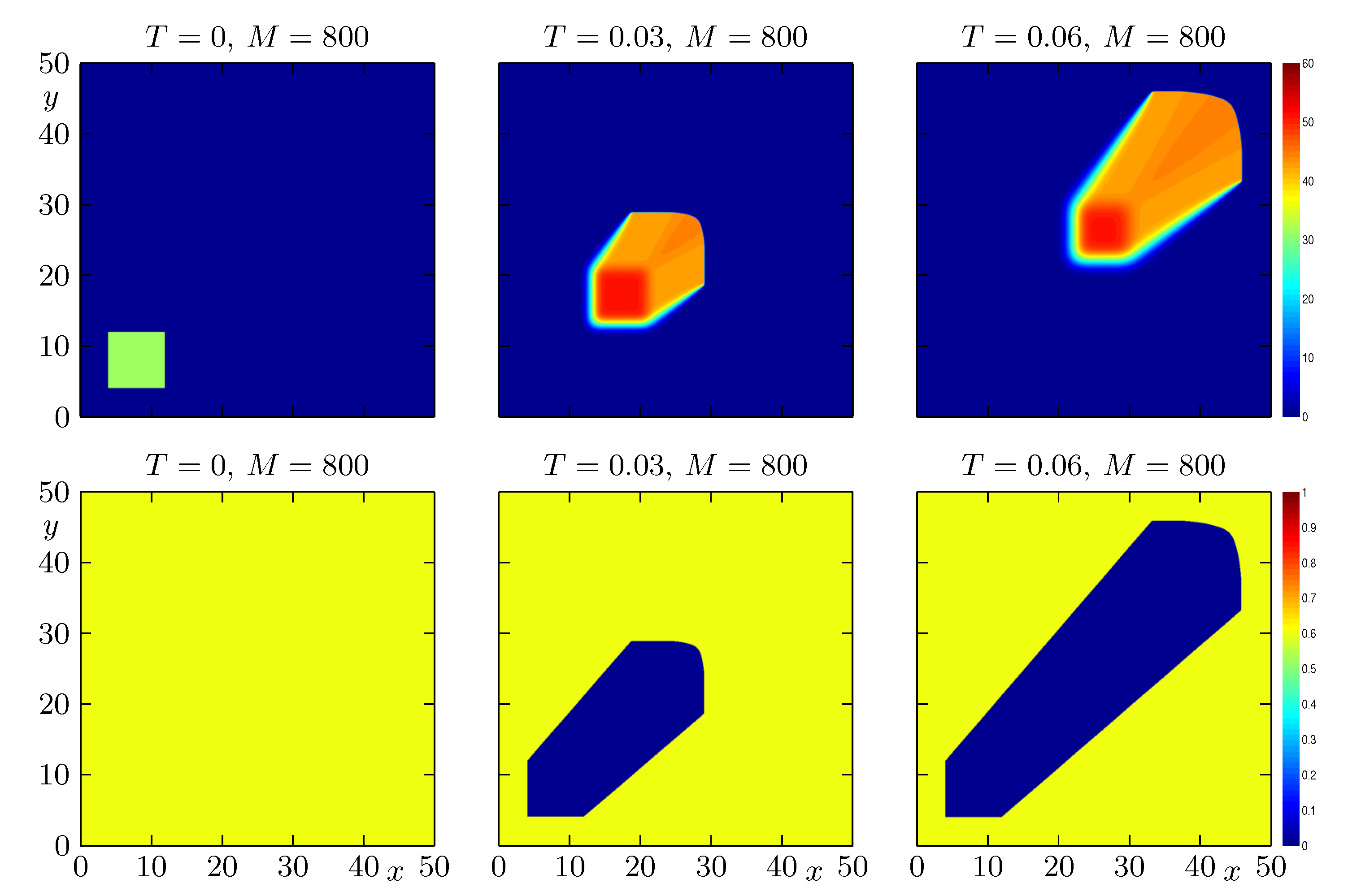
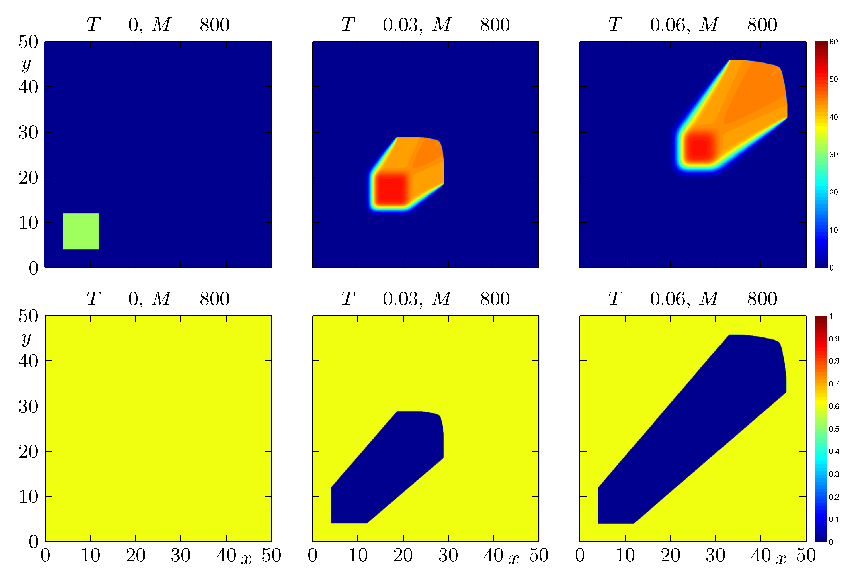
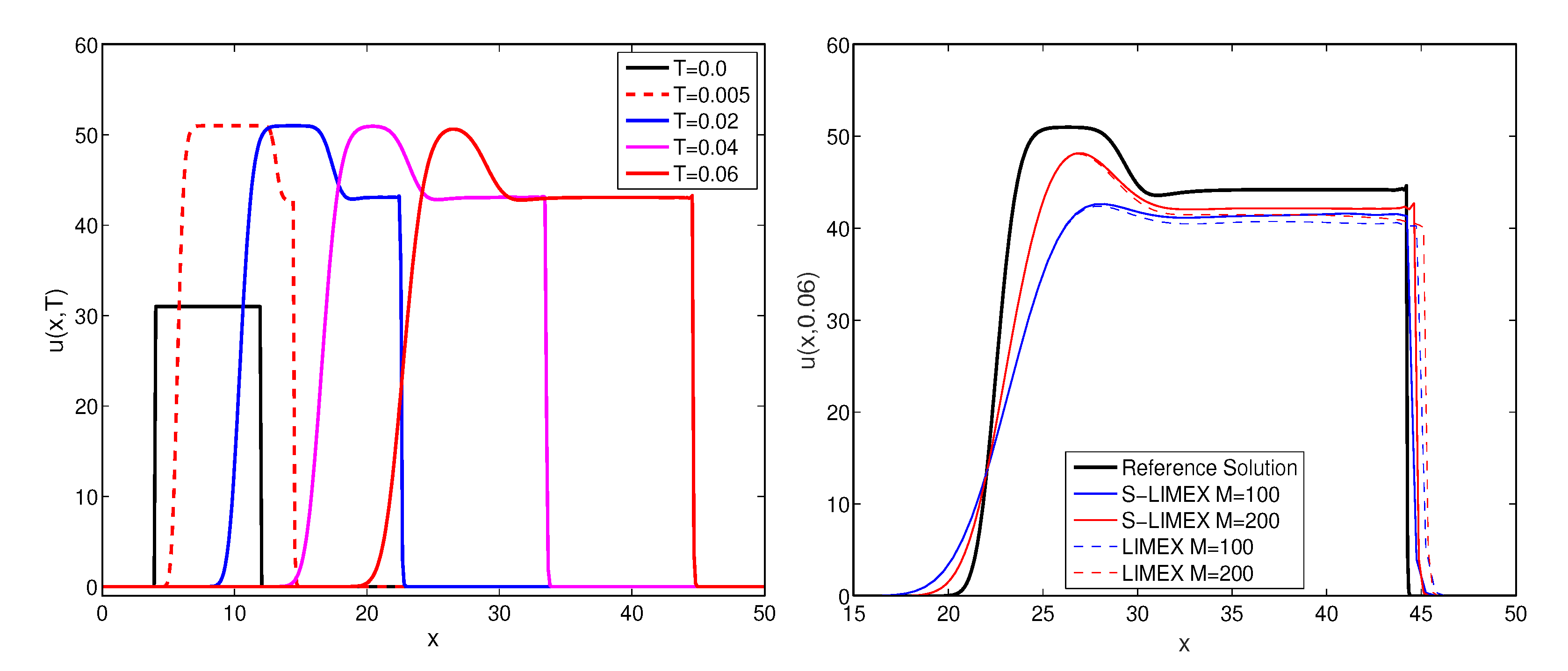
4.1. Example 1: Propagation of a Wildfire with Constant Initial Distribution of Fuel

In this example we compare the approximations obtained by both schemes, S-LIMEX and LIMEX, for different discretizations and simulated times. We consider first a configuration that allows us to compare our results with those of [1]. This means that we solve (1) on the domain $\mathsf{\Omega }$ with $L=50$ in dimensionless variables, which corresponds to a square of side length $50l_0=14.99\mathrm{m}$. We choose the dimensionless wind vector $\mathit{w}=(w_1,w_2)=(300,300)$, which blows in the north-east direction at physical speed $\parallel \mathit{v}\parallel =(l_0/t_0)\parallel \mathit{w}\parallel \approx 0.0142\mathrm{m}{\mathrm{s}}^{-1}$ (much larger values seem more realistic). The initial conditions for the non-dimensional temperature and the fuel are

$$u_0(x,y)=31{\chi }_{{[4,12]}^2}(x,y),v_0(x,y)=0.6{\chi }_{\mathsf{\Omega }}(x,y).$$

We display the numerical approximation obtained with both schemes in Figure 1 and Figure 2, with $\Delta x=\Delta y=50/400$ at simulated times $T=0.03$ and $T=0.06$, which represent $4.5$ and 9 minutes approximately. The dynamics of the propagation of wildfire is comparable with the results of [1]. In Figure 3(left) we display the evolution of the non-dimensional temperature within a short time interval on the diagonal $y=x$ of the domain $\mathsf{\Omega }$. The numerical approximation was computed with S-LIMEX scheme with $\Delta x=\Delta y=50/800$, corresponding to time step $\Delta t=7.8125\times {10}^{-6}$. The highest temperature reached during the initial steps does not exceed the maximum $U_{max}$ for the given parameters and initial conditions chosen. We also observe the formation of a fire front traveling in a direction parallel to $\mathit{w}$. In Figure 3(right) we compare the numerical approximation for both numerical schemes with respect to the reference solution for two discretization levels with $\Delta x=\Delta y=50/M$ for $M=100$ and $M=200$, corresponding to $\Delta t=6.25\times {10}^{-5}$ and $\Delta t=3.125\times {10}^{-5}$, respectively. Here we have represented the non-dimensional temperature at simulated time $T=0.06$ on the diagonal $y=x$. We observe that the numerical approximations are qualitatively equivalent. In

Table 1. Example 1: Approximate $L^1$ errors $e_M\left(u\right)$, $e_M\left(v\right)$ and CPU time.

	LIMEX			S-LIMEX
$\mathit{M}$	${\mathit{e}}_{\mathit{M}}\left(\mathit{u}\right)$	${\mathit{e}}_{\mathit{M}}\left(\mathit{v}\right)$	cpu[s]	${\mathit{e}}_{\mathit{M}}\left(\mathit{u}\right)$	${\mathit{e}}_{\mathit{M}}\left(\mathit{v}\right)$	cpu[s]
	$T=0.03$
50	2.32	2.1 $\times {10}^{-2}$	0.7	1.74	1.5 $\times {10}^{-2}$	0.3
100	1.22	1.8 $\times {10}^{-2}$	6.3	1.11	9.6 $\times {10}^{-3}$	3.5
200	0.96	1.1 $\times {10}^{-2}$	19.1	0.83	8.1 $\times {10}^{-3}$	18.8
400	0.59	6.3 $\times {10}^{-3}$	133.6	0.59	6.6 $\times {10}^{-3}$	162.0
800	0.27	3.3 $\times {10}^{-3}$	1012.6	0.32	3.8 $\times {10}^{-3}$	1405.0
	$T=0.06$
50	4.01	7.5 $\times {10}^{-2}$	3.2	2.99	3.8 $\times {10}^{-2}$	1.2
100	3.12	4.2 $\times {10}^{-2}$	13.3	2.54	3.3 $\times {10}^{-2}$	7.7
200	2.38	3.6 $\times {10}^{-2}$	38.6	2.05	2.8 $\times {10}^{-2}$	36.9
400	1.51	2.1 $\times {10}^{-2}$	266.6	1.51	2.2 $\times {10}^{-2}$	324.7
800	0.72	1.1 $\times {10}^{-2}$	2004.7	0.87	1.3 $\times {10}^{-2}$	2737.4

we compute the approximate $L^1$-errors $e_M\left(u\right)$ and $e_M\left(v\right)$ for both numerical schemes with different discretizations $\Delta x=\Delta y=50/M$ and $M=50,$ 100, 200, 400 and 800, with respect to a reference solution computed with S-LIMEX scheme with $M=3200$. For these cases, we employ $\Delta t=1.25\times {10}^{-4}$ for the coarse mesh and $\Delta t=7.8125\times {10}^{-6}$ for the finer mesh. We observe that for the coarse mesh, the S-LIMEX scheme is more accurate than the LIMEX scheme, however for a finer mesh, LIMEX is more accurate and faster than the S-LIMEX scheme.

On the other hand, to demonstrate that the proposed S-LIMEX scheme really provides an advantage, we consider an alternative scenario where $L=10$, $\mathit{w}=(1,1)$, and the initial conditions are

$$u_0(x,y)=31{\chi }_{{[1,5]}^2}(x,y),v_0(x,y)=0.7{\chi }_{\mathsf{\Omega }}(x,y)$$

with the same parameters as in the above scenario. For this configuration we compare two schemes: the S-LIMEX scheme and a scheme where all terms are discretized explicitly (Fully Explicit scheme). Since especially the last scheme entails very large computation times, we present results for fairly short simulation times only, namely $T=0.02$ and $T=0.03$. The scenario is of interest only in terms of accuracy and CPU times. The corresponding results, namely the approximate $L^1$-errors $e_M\left(u\right)$ and $e_M\left(v\right)$ and CPU times for these two methods are provided in

Table 2. Example 1, alternate scenario: Approximate $L^1$ errors $e_M\left(u\right)$ and $e_M\left(v\right)$ and CPU time for Strang LIMEX and Explicit schemes.

	S-LIMEX			Fully Explicit
$\mathit{M}$	${\mathit{e}}_{\mathit{M}}\left(\mathit{u}\right)$	${\mathit{e}}_{\mathit{M}}\left(\mathit{v}\right)$	cpu[s]	${\mathit{e}}_{\mathit{M}}\left(\mathit{u}\right)$	${\mathit{e}}_{\mathit{M}}\left(\mathit{v}\right)$	cpu[s]
	$T=0.02$
20	2.13	1.9 $\times {10}^{-2}$	0.1	2.51	2.1 $\times {10}^{-2}$	2868.6
40	1.57	1.4 $\times {10}^{-2}$	0.2	1.83	1.8 $\times {10}^{-2}$	7145.7
80	1.08	9.3 $\times {10}^{-3}$	0.5	1.17	1.3 $\times {10}^{-2}$	11,086.3
160	0.89	7.4 $\times {10}^{-3}$	3.6	0.99	8.5 $\times {10}^{-3}$	42,906.2
	$T=0.03$
20	2.32	2.5 $\times {10}^{-2}$	0.1	2.81	2.7 $\times {10}^{-2}$	5856.9
40	1.71	1.7 $\times {10}^{-2}$	0.2	2.54	2.1 $\times {10}^{-2}$	9854.2
80	1.19	1.3 $\times {10}^{-2}$	0.6	1.32	1.6 $\times {10}^{-2}$	16,823.7
160	0.94	9.7 $\times {10}^{-3}$	5.1	1.03	1.1 $\times {10}^{-2}$	65,305.5

. Here we compare the error of approximation with respect to a reference solution with $M_{\mathrm{ref}}=1280$ cells per dimension. According to Table 2, the errors and CPU times produced by the S-LIMEX scheme are smaller than the Fully Explicit scheme. This means that the S-LIMEX scheme is more efficient. Theoretical considerations support that the S-LIMEX scheme should become more efficient for sufficiently fine discretizations, but the results of Table 2 provide evidence that there is a clear gain in efficiency even for moderately fine discretizations (e.g., $M=40$ or $M=80$).

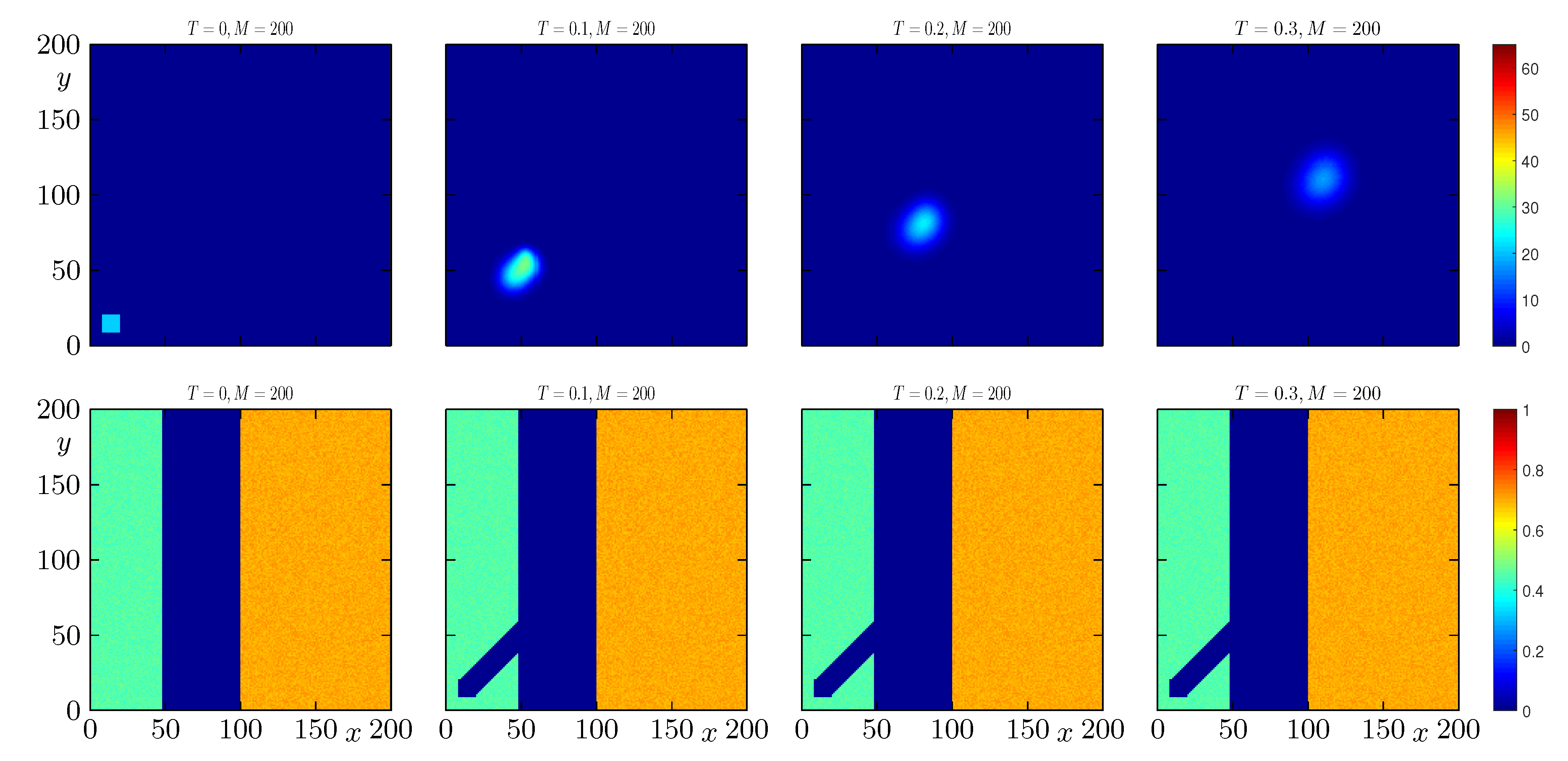
4.2. Example 2: Propagation of a Wildfire with Distribution of Fuel Determined by Two Areas with Different Fuel Densities

In this example we describe the dynamics of the wildfire when it enters a region with different fuel density. We consider $\mathsf{\Omega }:=(0,200)\times (0,200)$, $\epsilon =0.035$, $u_{\mathrm{pc}}=20$ and $\mathit{w}=(300,300)$. First, we employ the initial conditions

$$\begin{array}{c}\hfill u_0(x,y)=21{\chi }_{{[9,21]}^2}(x,y),v_0(x,y)=\left\{\begin{array}{cc}0.45+\delta (x,y)\hfill & \mathrm{for}x\le 100,\hfill \\ 0.70+\delta (x,y)\hfill & \mathrm{for}x>100,\hfill \end{array}\right.\end{array}$$

(15)

where $\delta$ is a function that is constant on each cell of the computational grid, and takes random values with $\left|\delta \right(x,y\left)\right|\le 0.025$. Notice that the initial density of fuel is higher for $x>100$ than for $x<100$. In Figure 4 we display the numerical solution at four simulated times, namely the initial condition at $T=0$ and the solution at $T=0.1$, $T=0.2$ and $T=0.3$. We observe that when the wildfire enters a region with higher fuel density, the non-dimensional temperature increases. Moreover, the width of the fire in the main direction of propagation is higher than in the less dense area, and this width increases with time and the fire opens.

Next we employ the same initial condition for temperature. However, to detect where the fire is extinguished when the availability of fuel is low, we impose

$$\begin{array}{c}\hfill v_0(x,y)=\left\{\begin{array}{cc}0.45\hfill & \mathrm{for}x\le 50,\hfill \\ 5\times {10}^{-4}\hfill & \mathrm{for}x>50.\hfill \end{array}\right.\end{array}$$

In Figure 5 we display the initial condition and the numerical solution at $T=0.1$, $T=0.2$ and $T=0.3$. We observe that when the wildfire enters a region with a very low fuel density, the fire focus width decreases with time and tends to disappear since the temperature of the focus remains below $u_{\mathrm{pc}}$ when it has already traveled more than 100 (unit lengths). This behavior allows one to identify the horizontal length after which the fire is extinguished (at the given wind speed). The numerical results in Figure 4 and Figure 5 were computed with S-LIMEX scheme with $\Delta x=\Delta y=200/M$ and $M=200$, corresponding to $\Delta t=1.25\times {10}^{-4}$.

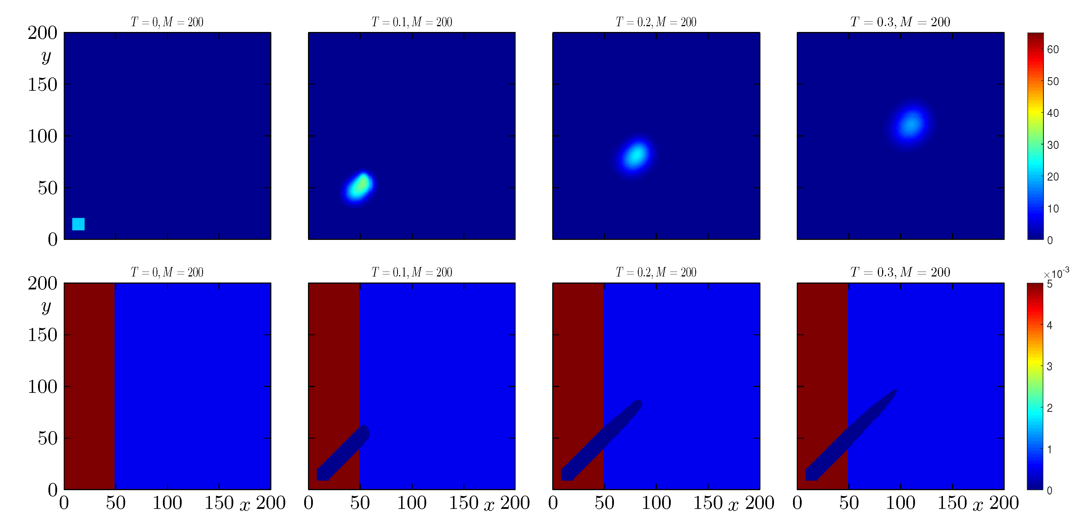
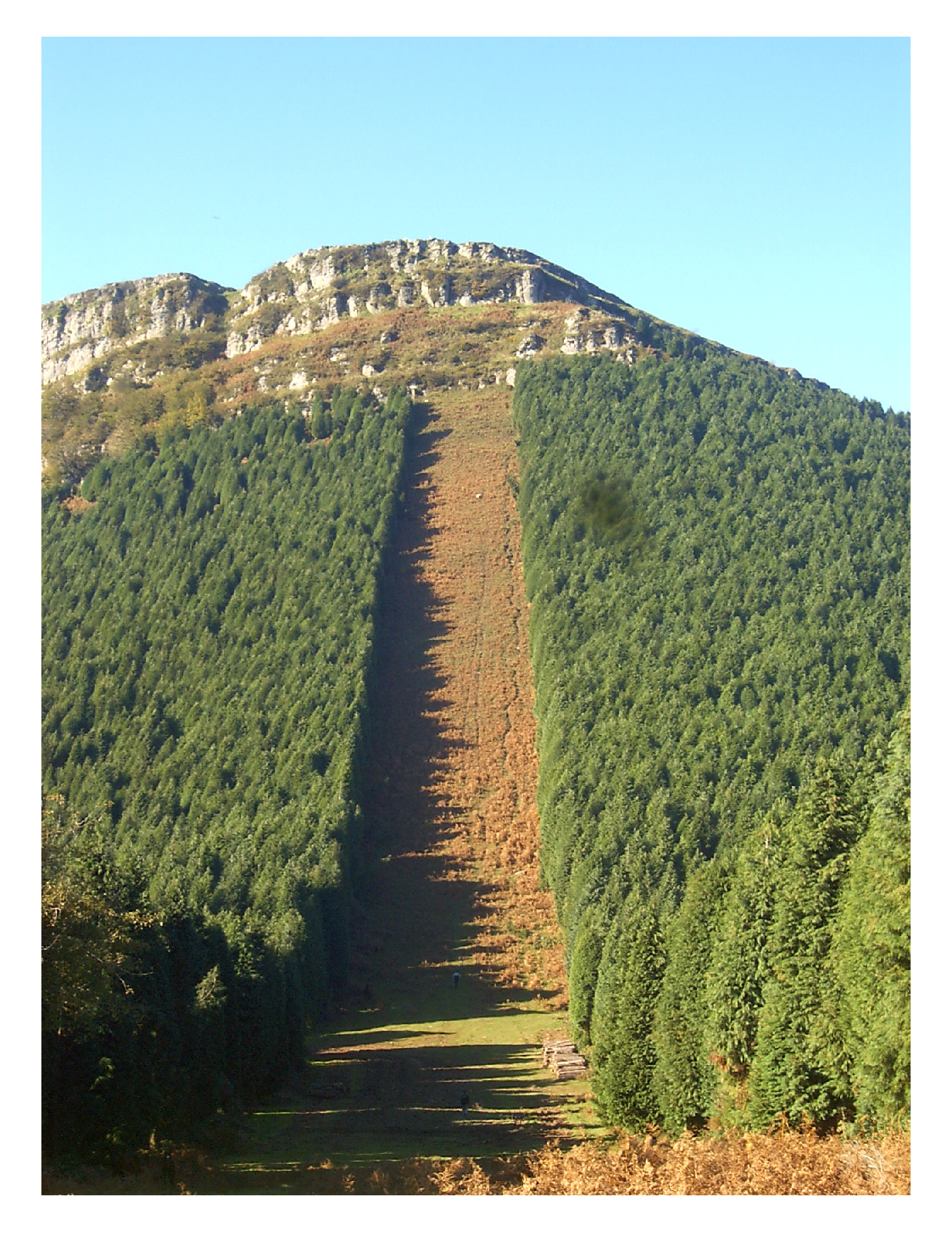
4.3. Example 3: Effect of a Firebreak in the Propagation of a Wildfire

In the prevention and control of forest fires, the role played by the implementation or construction of firebreaks (see Figure 6) is very important. Their role is to mitigate the effect of a fire or ideally prevent the spread of fire. This is usually done through the creation of a rectangular space void of fuel, that is in this case, of vegetation whose objective is to separate two zones to protect a certain area. Clearly, it is of great importance that one should be able to estimate the necessary width of the firebreak, as is pointed out in [14,15]. The protected area could be a forest with a large amount of fuel from which wood is obtained for commercial use, a native forest, or a set of households. To implement this fire control strategy using firebreaks, it is essential to study the effects that determine the width of said area with a fuel density close or equal to zero.

This situation motivates this third example where we study the effect of a firebreak in the propagation of a wildfire separating two areas with different fuel distribution. We consider the same parameters as in Example 2 with $u_0$ as in (15) and the initial distribution of fuel

$$v_0(x,y)=\left\{\begin{array}{cc}0.45+\delta (x,y)\hfill & \mathrm{for}x\le 100-l,\hfill \\ 0.7+\delta (x,y)\hfill & \mathrm{for}x>100,\hfill \end{array}\right.$$

where again the function $\delta$ is constant on each cell of the computational grid, and takes random values with $\left|\delta \right(x,y\left)\right|\le 0.025$. Moreover, $l>0$ is the width of the firebreak separating the two areas. Here we consider two cases, $l=25$ and $l=50$.

In the case $l=25$, we display in Figure 7 the dynamics of propagation of the wildfire at four simulated times. We observe that when the wildfire front crosses the firebreak region, the non-dimensional temperature decreases, however the wildfire does not extinguish and propagates into the area with high fuel density. Its temperature increases and the fire focus widens. In

Table 3. Example 3: Total amount of available (unburnt) fuel in the denser area at different times.

Time	$\mathit{l}=0$	$\mathit{l}=25$	$\mathit{l}=50$
$T=0.1$	14,000.93	14,000.93	14,000.93
$T=0.2$	13,826.65	14,000.93	14,000.93
$T=0.3$	12,699.81	12,956.04	14,000.93

we compute the total amount of fuel in the denser area for different widths of the firebreak. We observe that amount of fuel burnt for $l=25$ is smaller than for $l=0$, see also Figure 4 corresponding to the first part of Example 2. On the other hand, when $l=50$, we can see in Figure 8 that the wildfire is extinguished and does not propagate from the area with lower fuel density to that with higher density. These values of l are in accordance with those suggested by CONAF in its handbook [15].

The results obtained in these two scenarios agree with those of the second part of the previous example since there it can be seen that the temperature is below $u_{\mathrm{pc}}=20$ and remains so over time for $x<100$, which suggests that the width of the firebreak should be approximately 50 units of length. The numerical results of Figure 9 were computed by the S-LIMEX scheme with $\Delta x=\Delta y=200/M$ and $M=200$, corresponding to a time step $\Delta t=1.25\times {10}^{-4}$.

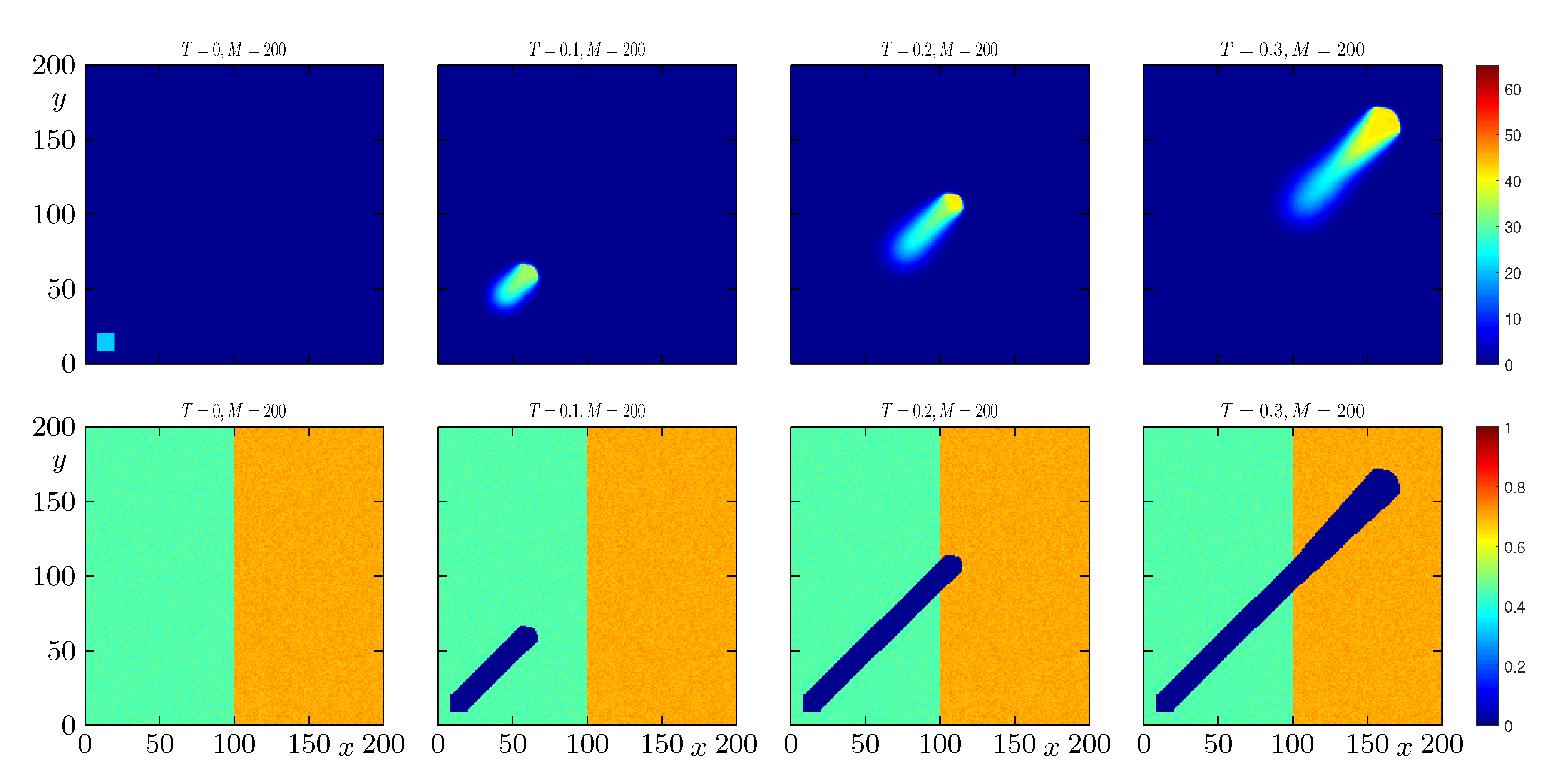
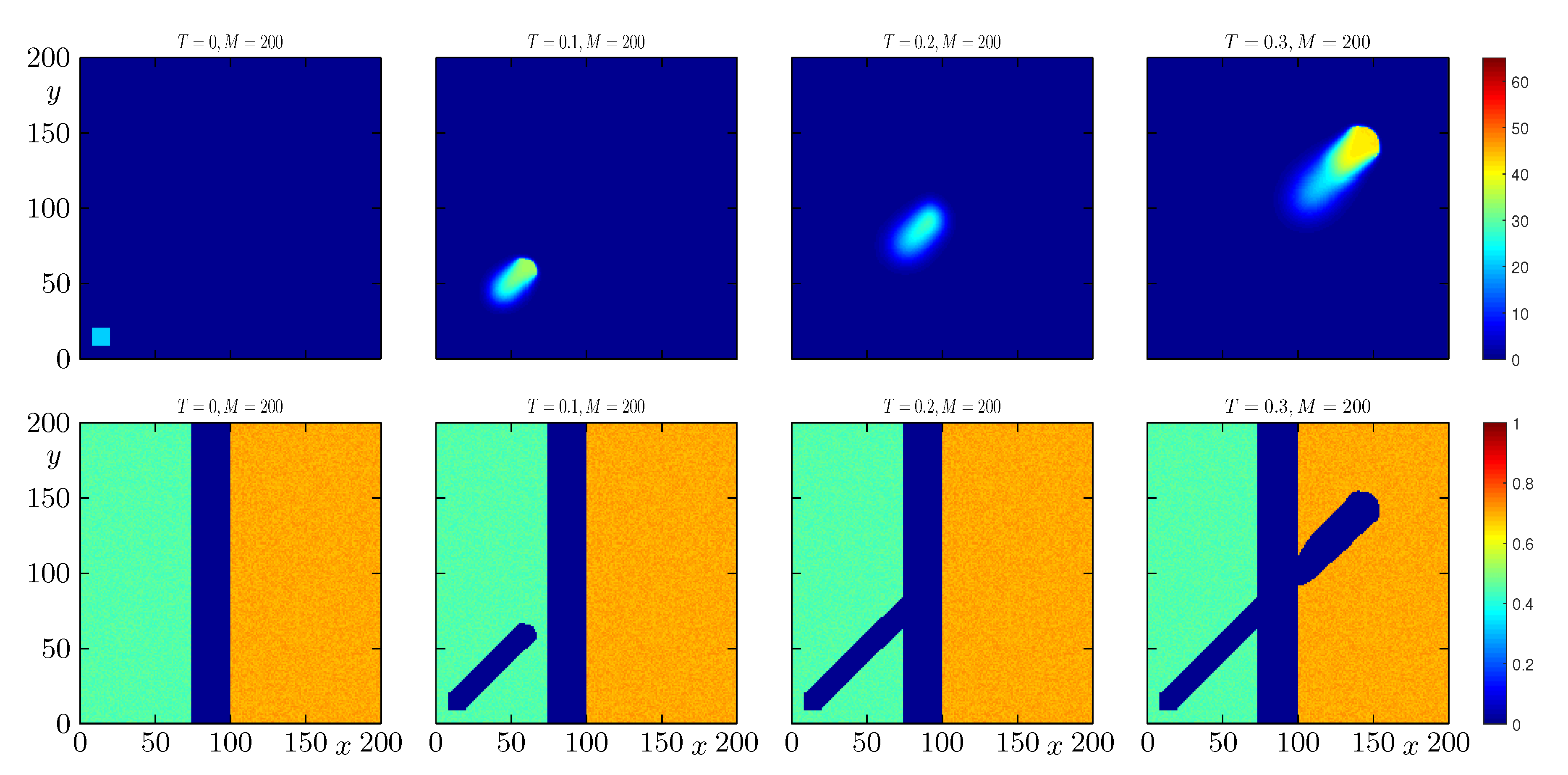
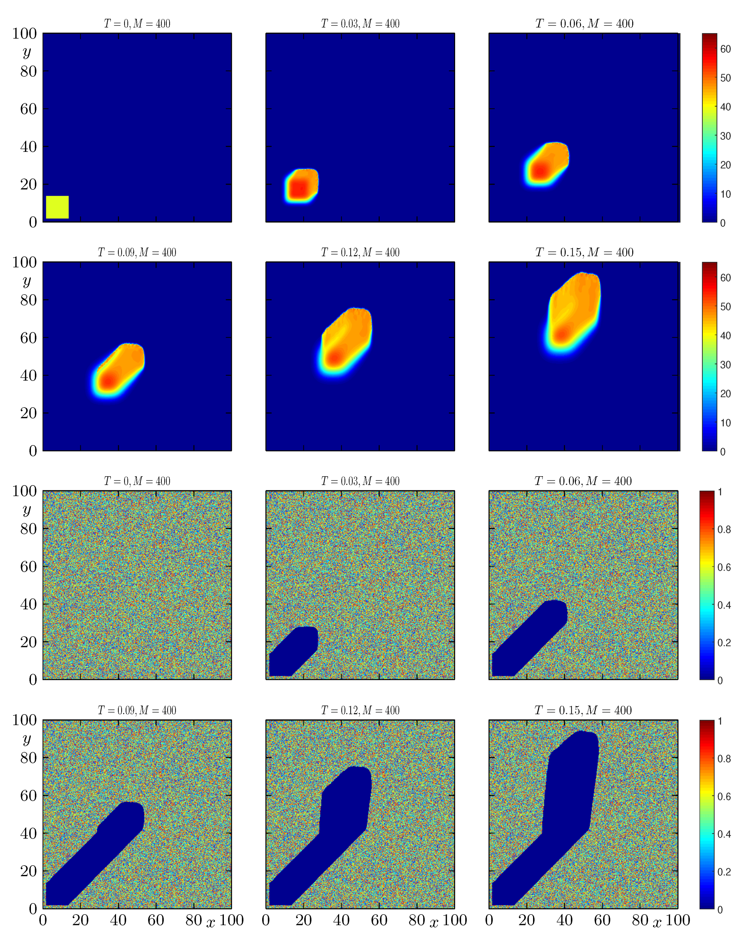
4.4. Example 4: Propagation of a Wildfire with Randomized Initial Distribution of Fuel and a Slight Change of Direction in the Wind

On a macroscopic scale, the wind direction is generally variable, but on a smaller scale and for a fixed region in the context of forest fires this direction can be considered constant or at most slightly variable only. In this configuration we consider $\mathsf{\Omega }$ with $L=200$ in dimensionless variables, which corresponds to a square of side length $200l_0=59.96\mathrm{m}$ with a randomized initial distribution of fuel in the whole domain. We choose initially the dimensionless initial wind vector $\mathit{w}=(300,300)$ and we change the wind direction at time $T=0.085$, which represents approximately 14 minutes, to ${\mathit{w}}^{*}=(50,400)$. We wish to observe the dynamics in the wildfire until simulated time $T=0.15$. The initial values for the non-dimensional temperature and the fuel distribution are

$$u_0(x,y)=38{\chi }_{{[2,14]}^2}(x,y),v_0(x,y)=0.5+\delta (x,y)$$

where $\delta$ is a function that is constant on each cell of the computational grid, and takes random values with $\left|\delta \right(x,y\left)\right|\le 0.4$.

In Figure 9 we can observe the effect of the change of the wind. From the initial time until before the simulated time $T=0.085$ it can be seen that the strip corresponding to the burnt fuel has a certain constant thickness and when the direction of the wind changes to ${\mathit{w}}^{*}$ we observe an increase in the width of the strip of the burnt area. The numerical results in Figure 9 were obtained by the S-LIMEX scheme with $\Delta x=\Delta y=100/M$ and $M=400$, corresponding to $\Delta t=6.25\times {10}^{-5}$.

5. Conclusions

We have implemented two numerical methods that allow studying the model defined by (4) and (5). The first method is a linearly implicit IMEX-RK scheme (denoted by “LIMEX”) and is described in Section 3.2. The second is a linearly implicit IMEX-RK method with Strang-type splitting (denoted by “S-LIMEX”) and is described in Section 3.3. Both methods allow us to study the evolution of the temperature and fuel variables over time based on certain initial conditions. In the first instance, we worked with both methods in order to study the evolution of numerical simulations such as those of Example 1. With respect to the original main research question on the gain of efficiency we mention that as Table 2 indicates, the S-LIMEX method is associated with significantly smaller CPU times, especially for fine discretizations of the computational domain in compare to the fully Explicit scheme. Concerning the secondary research question whether the model is indeed suitable for the simulation of wildfire control, we comment first that by considering a certain set of parameters we observe that the fire focus tends to move through the domain according to the direction of the wind speed and that given a certain constant fuel density, this focus increases as time passes. In Example 1 both methods are compared according to the projection of the fire front onto the diagonal of the domain.

To further demonstrate the practical applicability of the second numerical method we have designed a strategy, knowing that when the availability of fuel is very low then the wildfire tends to be extinguished by the effect of diffusion and convection. This property allows us to detect the horizontal distance that the fire front travels before it is completely extinguished. One may then build a firebreak in order to mitigate the effect of the fire or totally prevent its passage towards a certain area that has to be protected and thus avoid what is seen in one of the subcases of Example 2. Then considering the ideal width of said firebreak we proceed to compare two situations, one in which the width is less than the ideal and whose effect is partial in the sense that the fire does propagate into the area one is interested in protecting. The partiality of the effect becomes apparent in that only less fuel is consumed than in the case when the firebreak is absent (as is illustrated by Example 3), but the propagation of the fire is not stopped. On the other hand, when considering the ideal width we can see that this new firebreak does prevent the fire front from passing into the area that one wishes to protect. We have also studied what happens when a slight change in the direction of the wind occurs in a certain domain, which has the effect of considerably widening the width of the focus of the fire.

Clearly, our approach still exhibits a number of limitations. For the moment, and to focus on computational issues, we have considered idealized examples and no real-world scenarios, for which data of the terrain, vegetation, climate and wind effects would be required. Another omission is the neglect of moisture and pyrolysis effects. From a computational point of view, we mention that the present version of the Strang splitting method is still based on using a single time step for the whole computational domain. It could probably be made more efficient by local time stepping so that time-consuming small time steps are employed only where it is necessary.

Overcoming the limitations addressed above will be our main goal of future research. We mention first that our interest in the wildfire propagation model (1) is partially motivated by experience with IMEX methods for related applicative nonlinear convection-diffusion problems. These methods achieve a considerable gain of efficiency compared with easier-to-implement explicit schemes, but require the solution of linear or nonlinear systems of algebraic equations. The results presented herein are basically encouraging and reconfirm that the model can in principle be used for the prediction of wildfire propagation and its mitigation through cutting firebreaks of sufficient width. However, future research is still necessary to establish IMEX methods as a really competitive tool for wildfire simulation. One aspect is related to the discretization of the reaction terms. Another future research direction points at incorporating further model ingredients. These include topography of the terrain (as expressed by the function $h\left(\mathit{x}\right)$ that describes spatial heterogeneity but which has been chosen constant here; see Section 2.2), as well as radiation, moisture content and pyrolysis via a multivalued enthalpy function.

Finally, we remark that as the discussion of Section 1.1 and Section 1.2 shows, a considerable number of variants of the model (4), (5), as originally proposed in [1], have appeared along with a great variety of numerical methods. All these models refer to realities that vary drastically between different geographic regions, types of vegetation and climate. Moreover forecasts are sought on spatial and temporal scales that differ substantially from case to case. Thus, a comprehensive comparison of the models and their discretizations should start with the definition of a unique “benchmark” scenario for numerical testing that could be handled by all of them. This endeavor is, however, outside the scope of this paper.

References

1. Asensio, M.I.; Ferragut, L. On a wildland fire model with radiation. Int. J. Numer. Meth. Engrg. 2002, 54, 137–157. [Google Scholar] [CrossRef]
2. LeVeque, R.J. Finite Volume Methods for Hyperbolic Problems; Cambridge University Press: Cambridge, UK, 2002. [Google Scholar]
3. Boscarino, S.; Bürger, R.; Mulet, P.; Russo, G.; Villada, L.M. Linearly implicit IMEX Runge-Kutta methods for a class of degenerate convection-diffusion problems. SIAM J. Sci. Comput. 2015, 37, B305–B331. [Google Scholar] [CrossRef]
4. Boscarino, S.; Bürger, R.; Mulet, P.; Russo, G.; Villada, L.M. On linearly implicit IMEX Runge-Kutta Methods for degenerate convection-diffusion problems modelling polydisperse sedimentation. Bull. Braz. Math. Soc. (New Ser.) 2016, 47, 171–185. [Google Scholar] [CrossRef]
5. Boscarino, S.; Filbet, F.; Russo, G. High order semi-implicit schemes for time dependent partial differential equations. J. Sci. Comput. 2016, 68, 975–1001. [Google Scholar] [CrossRef] [Green Version]
6. Boscarino, S.; LeFloch, P.G.; Russo, G. High order asymptotic-preserving methods for fully nonlinear relaxation problems. SIAM J. Sci. Comput. 2014, 36, A377–A395. [Google Scholar] [CrossRef]
7. Bürger, R.; Chowell, G.; Gavilán, E.; Mulet, P.; Villada, L.M. Numerical solution of a spatio-temporal gender-structured model for hantavirus infection in rodents. Math. Biosci. Eng. 2018, 15, 95–123. [Google Scholar] [CrossRef] [PubMed] [Green Version]
8. Bürger, R.; Chowell, G.; Gavilán, E.; Mulet, P.; Villada, L.M. Numerical solution of a spatio-temporal predator-prey model with infected prey. Math. Biosci. Eng. 2019, 16, 438–473. [Google Scholar] [CrossRef] [PubMed]
9. Bürger, R.; Inzunza, D.; Mulet, P.; Villada, L.M. Implicit-explicit schemes for nonlinear nonlocal equations with a gradient flow structure in one space dimension. Numer. Methods Partial Differ. Equ. 2019, 35, 1008–1034. [Google Scholar] [CrossRef]
10. Bürger, R.; Inzunza, D.; Mulet, P.; Villada, L.M. Implicit-explicit methods for a class of nonlinear nonlocal gradient flow equations modelling collective behaviour. Appl. Numer. Math. 2019, 144, 234–252. [Google Scholar] [CrossRef]
11. Bürger, R.; Mulet, P.; Villada, L.M. Regularized nonlinear solvers for IMEX methods applied to diffusively corrected multi-species kinematic flow models. SIAM J. Sci. Comput. 2013, 35, B751–B777. [Google Scholar] [CrossRef]
12. Butcher, J.C. Numerical Methods for Ordinary Differential Equations, 2nd ed.; Wiley: Chichester, UK, 2008. [Google Scholar]
13. Donat, R.; Guerrero, F.; Mulet, P. Implicit-explicit methods for models for vertical equilibrium multiphase flow. Comput. Math. Appl. 2014, 68, 363–383. [Google Scholar] [CrossRef]
14. Generalitat Valenciana. Manual of Good Practices in Forest Fires Prevention. Available online: http://www.agroambient.gva.es/documents/162905929/162908886/Manual+de+Buenas+Pr%C3%A1cticas+en+Prevenci%C3%B3n+de+Incendios+Forestales+-+English+%28383%2C2k%29/65f00043-102a-4835-a129-0b4bd364df79 (accessed on 1 April 2020).
15. Ortega, M. Manual Medidas Prediales de Protección Contra Incendios Forestales; Documento de trabajo 451; Corporación Nacional Forestal: Antofagasta, Chile, 2006. [Google Scholar]
16. Pastor, E.; Zárate, L.; Planas, E.; Arnaldos, J. Mathematical models and calculation systems for the study of wildland fire behaviour. Progr. Energy Combust. Sci. 2003, 29, 139–153. [Google Scholar] [CrossRef]
17. Eberle, S.; Freeden, W.; Matthes, U. Forest fire spreading. In Handbook of Geomathematics, 2nd ed.; Freeden, W., Nashed, M.Z., Sonar, T., Eds.; Springer-Verlag: Berlin, Germany, 2015; pp. 1349–1385. [Google Scholar]
18. San Martín, D.; Torres, C.E. Ngen-Kütral: Toward an open source framework for Chilean wildfire spreading. In Proceedings of the 37th International Conference of the Chilean Computer Science Society (SCCC), Santiago, Chile, 5–9 November 2018; pp. 1–8. [Google Scholar]
19. Ferragut, L.; Asensio, M.I.; Monedero, S. Modelling radiation and moisture content in fire spread. Commun. Numer. Meth. Engrg. 2007, 23, 819–833. [Google Scholar] [CrossRef]
20. Ferragut, L.; Asensio, M.I.; Monedero, S. A numerical method for solving convection-reaction-diffusion multivalued equations in fire spread modelling. Adv. Engrg. Softw. 2007, 38, 366–371. [Google Scholar] [CrossRef]
21. Prieto, D.; Asensio, M.I.; Ferragut, L.; Cascón, J.M.; Morillo, A. A GIS-based fire spread simulator integrating a simplified physical wildland fire model and a wind field model. Int. J. Geograph. Inf. Sci. 2017, 31, 2142–2163. [Google Scholar] [CrossRef]
22. San Martín, D.; Torres, C.E. Exploring a spectral numerical algorithm for solving a wildfire mathematical model. In Proceedings of the 38th International Conference of the Chilean Computer Science Society (SCCC), Concepción, Chile, 4–9 November 2019; pp. 1–7. [Google Scholar]
23. Barovik, D.; Taranchuk, V. Mathematical modelling of running crown forest fires. Math. Model. Anal. 2010, 15, 161–174. [Google Scholar] [CrossRef] [Green Version]
24. Taranchuk, V.; Barovik, D. Numerical modeling of surface forest fire spread in nonuniform woodland. In Computer Algebra Systems in Teaching and Research Vol. VIII; Prokopenya, A.N., Gil-Świderska, A., Siłuszyk, M., Eds.; Siedlce University of Natural Sciences and Humanities, Institute of Mathematics and Physics: Siedlce, Poland, 2019; pp. 159–168. [Google Scholar]
25. Pareschi, L.; Russo, G. Implicit-Explicit Runge-Kutta schemes and applications to hyperbolic systems with relaxation. J. Sci. Comput. 2005, 25, 129–155. [Google Scholar]
26. Glassman, I.; Yetter, R.A.; Glumac, N.G. Combustion, 5th ed.; Academic Press: Boston, MA, USA, 2015. [Google Scholar]
27. Abgrall, R.; Shu, C.-W. Handbook of Numerical Analysis for Hyperbolic Problems. Basic and Fundamental Issues; North-Holland: Amsterdam, The Netherlands, 2016. [Google Scholar]
28. Hesthaven, J.S. Numerical Methods for Conservation Laws; Society for Industrial and Applied Mathematics: Philadelphia, PA, USA, 2018. [Google Scholar]
29. Holden, H.; Karlsen, K.H.; Lie, K.-A.; Risebro, N.H. Splitting Methods for Partial Differential Equations with Rough Solutions; European Mathematical Society: Zurich, Switzerland, 2010. [Google Scholar]
Figure 1. Example 1: Evolution of the dynamics of temperature (top) and fuel (bottom). Numerical approximation with S-LIMEX for Δ x = Δ y = 50 / 800 .
Mathematics 08 01034 g001
Figure 2. Example 1: Evolution of the dynamics of temperature (top) and fuel (bottom). Numerical approximation with LIMEX for Δ x = Δ y = 50 / 800 .
Mathematics 08 01034 g002
Figure 3. Example 1: 1-D projection of the numerical solution onto the line y = x : (left) evolution of the non-dimensional temperature during short time intervals, (right) comparison of the numerical approximations (with M = 200 and M = 400 at time T = 0.16 ) obtained by LIMEX and S-LIMEX schemes with the reference solution.
Mathematics 08 01034 g003
Figure 4. Example 2: Evolution of the dynamics of temperature (top) and fuel (bottom). Simulation when the wildfire enters a region with higher fuel density.
Mathematics 08 01034 g004
Figure 5. Example 2: Evolution of the dynamics of temperature (top) and fuel (bottom). Simulation when the wildfire enters a region with a very low fuel density.
Mathematics 08 01034 g005
Figure 6. An example of a firebreak (see https://es.wikipedia.org/wiki/Archivo:Eretza_2.jpg).
Mathematics 08 01034 g006
Figure 7. Example 3: Evolution of the dynamics of temperature (top) and fuel (bottom). Propagation of fire across a firebreak of insufficient width.
Mathematics 08 01034 g007
Figure 8. Example 3: Evolution of the dynamics of temperature (top) and fuel (bottom). Extinction of fire by a sufficiently wide firebreak.
Mathematics 08 01034 g008
Figure 9. Example 4: Evolution of the dynamics of temperature (top) and fuel (bottom). Evolution of the non-dimensional temperature and proportion of fuel in space under a change of the wind direction.
Mathematics 08 01034 g009