Article

Group Invariant Solutions and Conserved Quantities of a (3+1)-Dimensional Generalized Kadomtsev–Petviashvili Equation

by
Innocent Simbanefayi
1 and
Chaudry Masood Khalique
1,2,3,*
1
International Institute for Symmetry Analysis and Mathematical Modelling, Department of Mathematical Sciences, North-West University, Mafikeng Campus, Private Bag X 2046, Mmabatho 2735, South Africa
2
College of Mathematics and Systems Science, Shandong University of Science and Technology, Qingdao 266590, China
3
Department of Mathematics and Informatics, Azerbaijan University, Jeyhun Hajibeyli str., 71, Baku AZ1007, Azerbaijan
*
Author to whom correspondence should be addressed.
Mathematics 2020, 8(6), 1012; https://doi.org/10.3390/math8061012
Submission received: 13 May 2020 / Revised: 8 June 2020 / Accepted: 10 June 2020 / Published: 20 June 2020
(This article belongs to the Special Issue Recent Advances in Differential Equations and Applications)

Abstract

:
In this work, we investigate a (3+1)-dimensional generalised Kadomtsev–Petviashvili equation, recently introduced in the literature. We determine its group invariant solutions by employing Lie symmetry methods and obtain elliptic, rational and logarithmic solutions. The solutions derived in this paper are the most general since they contain elliptic functions. Finally, we derive the conserved quantities of this equation by employing two approaches—the general multiplier approach and Ibragimov’s theorem. The importance of conservation laws is explained in the introduction. It should be pointed out that the investigation of higher dimensional nonlinear partial differential equations is vital to our perception of the real world since they are more realistic models of natural and man-made phenomena.

1. Introduction

The study of nonlinear partial differential equations (NLPDEs) and their solutions has become a subject of much interest in the past few decades. Modelling natural phenomena such as the behaviour of water waves is often an interdisciplinary research area connecting such areas as mathematics, physics and engineering. Along with the progress in modelling nonlinear phenomena came a myriad of methods designed to derive the exact solutions of these models. Some of these methods are Lie group analysis [1,2,3,4,5], homogeneous balance technique [6], the ansatz method [7], the Hirota bilinear method [8], the ( G / G ) -expansion technique [9,10], the Kudryashov method [11,12], the simplest equation method [13], the Jacobi elliptic function expansion technique [14], and the F-expansion method [15], bifurcation method [16] just to mention a few.
The (3+1)-dimensional Kadomtsev–Petviashvili (KP) equations [17]
( u t + 6 u u x + u x x x ) x ± 3 u y y ± 3 u z z = 0
have their origins in the classic 1970 work of two Soviet physicists Kadomtsev and Petviashvili [18]. It models waves in scenarios where the ratio between the depth of water and the wavelength is very small coupled with insubstantial nonlinear restoring forces. It is also a generalisation of the Korteweg–de Vries (KdV) equation, named after the Dutch mathematicians Korteweg and de Vries [19]. The highest order term u x x x caters for weak dispersion, while the term u u x describes the nonlinearity aspect of a wave and the last two terms of (1) describe diffractive divergence [20]. The sign “±" in the last two terms corresponds to either positive or negative dispersion. Since then, several researchers have studied equations of the form (1), see for instance [21,22,23,24,25,26]. Investigations into (1) have ranged from establishing the stability of their solitons [23], determining their integrability properties [24], Painlevé analysis [25] and deriving their exact multiple wave solutions [26]. The (3+1)-dimensional generalised KP equation
u t x + u t y + 3 u x u x y + 3 u x x u y + u x x x y u z z = 0
to the best of our knowledge was introduced in [27], where the Plücker relation for determinants was used to obtain one Wronskian solution. Furthermore, in the same work, the Jacobi identity for determinants was used to establish a Grammian solution for (2). Multiple solitons and multiple singular solitons for Equation (2) were derived in [28] using a simplified form of Hirota’s method. In their work, the researchers in [28] contrast their results with those obtained in [27] in terms of the spatial variable z. Later in [29], an extra term u t z , was added to (2), thus introducing a new form of the (3+1)-dimensional generalised KP equation, which we denote here by (3+1)-D gKPe, and it reads
u t x + u t y + u t z + 3 u x u x y + 3 u x x u y + u x x x y u z z = 0 .
In their work [29], the authors showed that addition of the new term affects the dispersion relations significantly. Furthermore, they applied Hirota’s direct method to determine the multiple soliton solutions of (3). In [30], the Equation (3) was studied and exact solutions were obtained through the use of Hirota’s bilinear method and an extended homoclinic test approach.
In this work, we seek to derive the exact solutions of the (3+1)-D gKPe (3) by making use of its Lie point symmetries and direct integration. We will not employ adhoc methods as often is the case when treating NLPDEs of this nature. Furthermore, we will for the first time derive the conserved quantities of Equation (3) by invoking two approaches.
Lie group theory was discovered by a Norwegian mathematician, Marius Sophus Lie (1842–1899), around the middle of nineteenth century. Lie perceived that the seemingly different methods for finding exact solutions of differential equations were, in reality, all special cases of a broad integration approach; the theory of transformation groups. This theory is an analog of Galois theory and has an enormous impact on mathematics and mathematical physics today. It is contemplated to be one of the most significant techniques to determine the exact solutions of differential equations [1,2,3,4,5].
Conservation laws are essential to our comprehension of the physical world and are considered to be basic laws of nature, with wide application in physics, and in other fields for instance chemistry, engineering, and so on. In classical physics, three types of such laws are conservation of energy, linear momentum and angular momentum. Conservation laws are used in establishing the integrability of differential equations (DEs) and are also used in determining whether the solution of a DE exists and is unique. Moreover, one can also use conservation laws in checking the authenticity of numerical solution methods [31,32,33,34,35,36,37,38,39,40,41,42,43,44].
We want to emphasize here that a study of higher dimensional NLPDEs is critical to our understanding of the world around us since they are more realistic models of natural and man-made phenomena [45].

2. Exact Solutions of the (3+1)-D gKPe

In this section, we determine the exact solutions of the (3+1)-D gKPe (3) by utilizing its Lie point symmetries and direct integration. Roughly speaking, a Lie point symmetry of a PDE is a local group of transformations acting on the independent and dependent variables of the PDE that maps every solution of the PDE to another solution of the same PDE. That is to say, it maps the solution set of the PDE to itself.
It can be seen, using for example, MathLie package [46], that Equation (3) has a finite-dimensional Lie subalgebra L 6 , which is generated by the vector fields
X 1 = t , X 2 = x , X 3 = y , X 4 = z , X 5 = t t + z x + z y + ( 2 t + z ) z , X 6 = 15 t t + 3 ( 4 t + x ) x + 3 ( 3 y 2 z ) y 3 ( 4 t z ) z + ( 4 x + 4 y 3 u ) u ,
and the two infinite-dimensional subalgebras generated by
X F 1 = F 1 ( t ) u , X F 2 = F 2 ( t + z ) u ,
where F 1 and F 2 are arbitrary functions of their arguments.

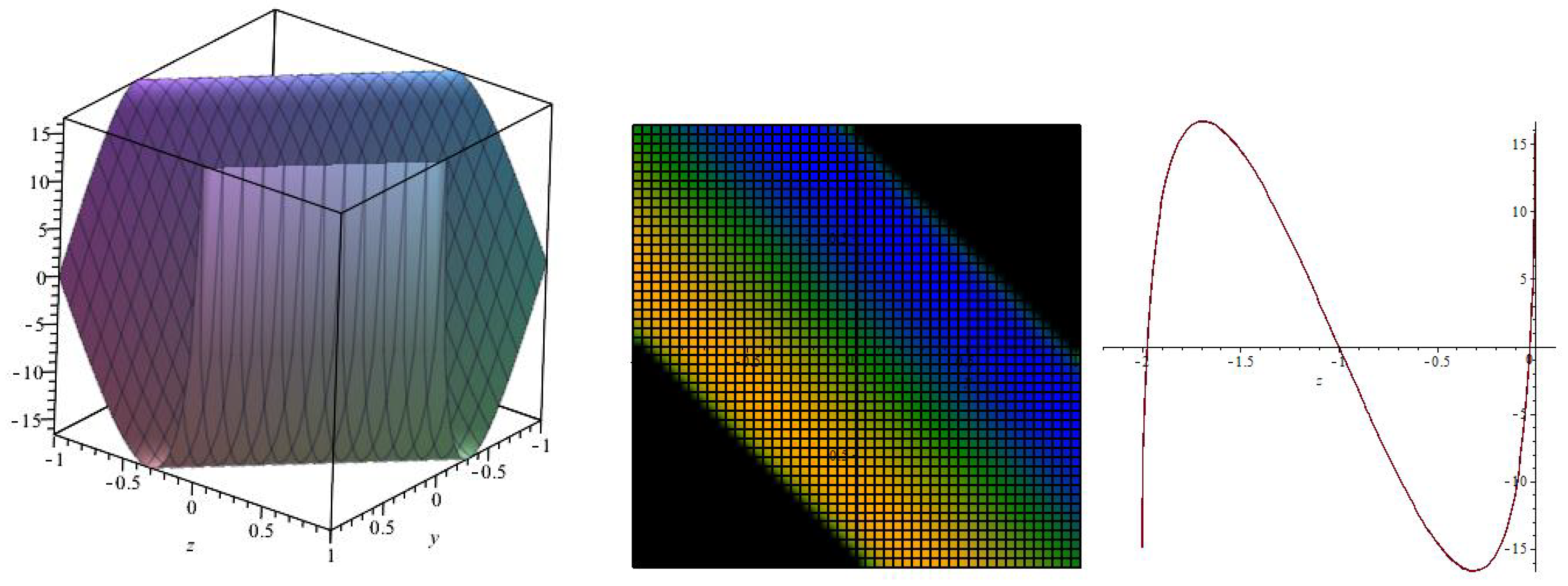
2.1. Invariant Solutions under the Symmetries X 1 , ⋯, X 4

Firstly, we invoke the translation symmetries and reduce the (3+1)-D gKPe (3) to a fourth order ordinary differential equation (ODE). Thus, using the four translation symmetries X 1 , X 2 , X 3 and X 4 of Equation (3), we can obtain the following invariant solution:
u ( t , x , y , z ) = U ( p ) , p = γ x + α y + β z ν t ,
where γ , α , β and ν are constants. This reduces the Equation (3) to
α γ 3 U + 6 α γ 2 U U ( α ν + β 2 + β ν + γ ν ) U = 0 .
Integrating (7) once with respect to p yields
α γ 3 U + 3 α γ 2 U 2 ( α ν + β 2 + β ν + γ ν ) U + K 0 = 0
with K 0 a constant. Now letting
U ( p ) = γ ϕ ( p ) , ω = α ν + β 2 + β ν + γ ν α γ 3 and K 1 = K 0 α γ 4 ,
Equation (8) becomes
ϕ + 3 ϕ 2 ω ϕ + K 1 = 0 .
This ODE can be integrated easily. Multiplying (9) by ϕ and integrating once with respect to p gives
ϕ 2 = ( 2 ϕ 3 ω ϕ 2 + 2 K 1 ϕ + 2 K 2 )
with K 2 an integration constant. If the algebraic equation ϕ 3 1 2 ω ϕ 2 + K 1 ϕ + K 2 = 0 has the roots λ 1 λ 2 λ 3 , then we have
ϕ 2 = 2 ( ϕ λ 1 ) ( ϕ λ 2 ) ( ϕ λ 3 ) .
Equation (11) has the well-known solution expressed in terms of the Jacobi elliptic function, that is,
ϕ ( p ) = λ 2 + ( λ 1 λ 2 ) cn 2 λ 1 λ 3 2 p M 2 , M 2 = λ 1 λ 2 λ 1 λ 3 .
Here cn ( p | M 2 ) is the Jacobi elliptic cosine function. Furthermore, pertinent to note is that when M 2 → 1, cn ( p | M 2 ) sech ( p ) and when M 2 → 0, cn ( p | M 2 ) cos ( p ) [47]. A comparison of Equations (9) and (10) reveals that
ω = 2 ( λ 1 + λ 2 + λ 3 ) , K 1 = λ 1 λ 2 + λ 2 λ 3 + λ 1 λ 3 , K 2 = λ 1 λ 2 λ 3 .
Reverting to original variables, the solution of the (3+1)-D gKPe (3) is thus
u ( t , x , y , z ) = { λ 2 ( 1 M 2 ) λ 1 } p M 2 + λ 1 λ 2 dn A p | M 2 E am A p | M 2 | M 2 A M 2 dn A p | M 2 2 ,
where E ( p | M 2 ) is the elliptic integral of the second kind, am ( p | M 2 ) is the amplitude function, dn ( p | M 2 ) is the delta amplitude function, cn ( p | M 2 ) is the Jacobi cosine function and A = ( λ 1 λ 3 ) / 2 [47,48]. Figure 1 depicts the profile of solution (13) for suitable parameter values.
Figure 1 depicts the coexistence of bright and dark solitons. It is well-known that bright soliton profile are characterized by hyperbolic secant. The bright soliton solution usually takes a bell-shaped figure and propagate undistorted without any change in shape for arbitrarily long distances. However, dark soliton solutions, configured also as topological optical solitons, are given by hyperbolic tangent.
Important to note is that Equation (10) is reminiscent of the ODE obtained in the quintessential work of Korteweg and de Vries in [49]. This ODE is associated with long waves propagating along a rectangular canal. The ODE (10) describes stationary waves and by imposing certain constraints such as having the fluid undisturbed at infinity, Korteweg and de Vries obtained negative and positive solitary waves as well as cnoidal wave solutions [49,50].

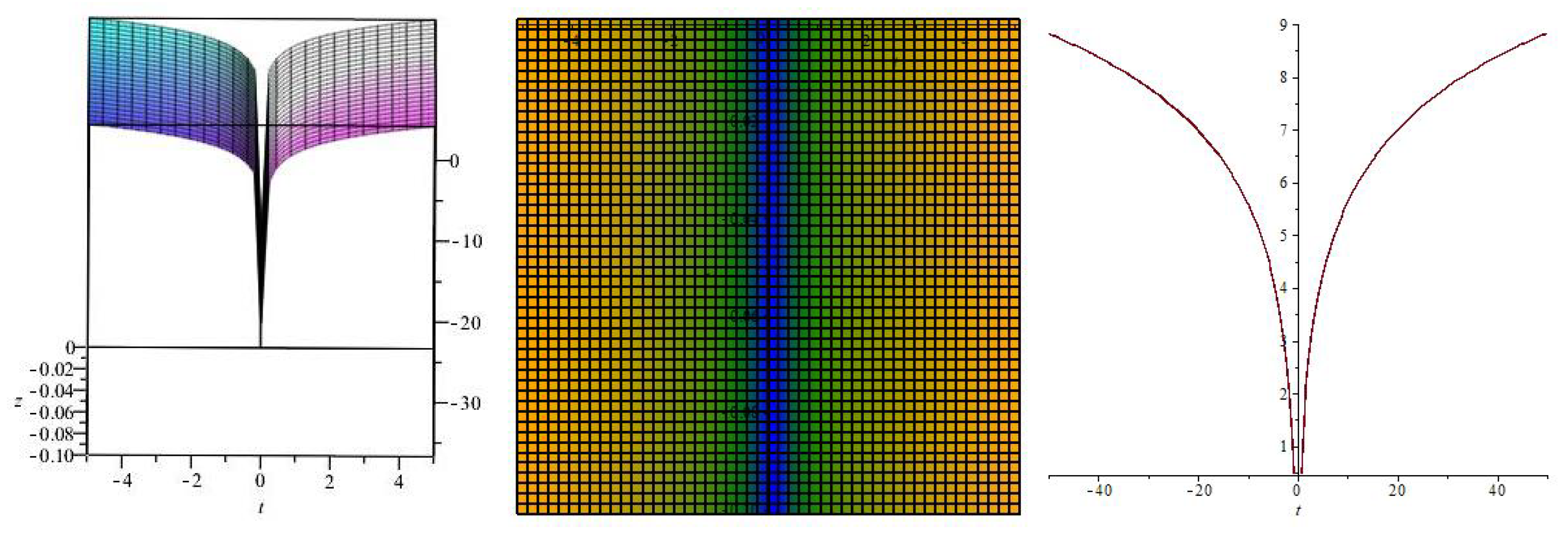
2.2. Invariant Solution under the Symmetry X 5

We now turn our attention to the point symmetry X 5 . The usual computations yield the group invariant solution u ( t , x , y , z ) = U ( ξ ) , where ξ = t ( t + z ) . This, substituted into (3) gives the ODE
ξ U + U = 0 ,
whose solution is U ( ξ ) = C 1 + C 2 ln ( ξ ) , and hence the group invariant solution of the (3+1)-D gKPe (3) under the symmetry X 5 is
u ( t , x , y , z ) = C 1 + C 2 ln t ( t + z )
with C 1 , C 2 integration constants. The corresponding graphical representation of solution (15) is given in Figure 2.
The profiles portrayed in Figure 2 are typical of a grey singular soliton solution, more so the distinctive asymptotic form observable for lim t 0 u ( t , x , y , z ) = .

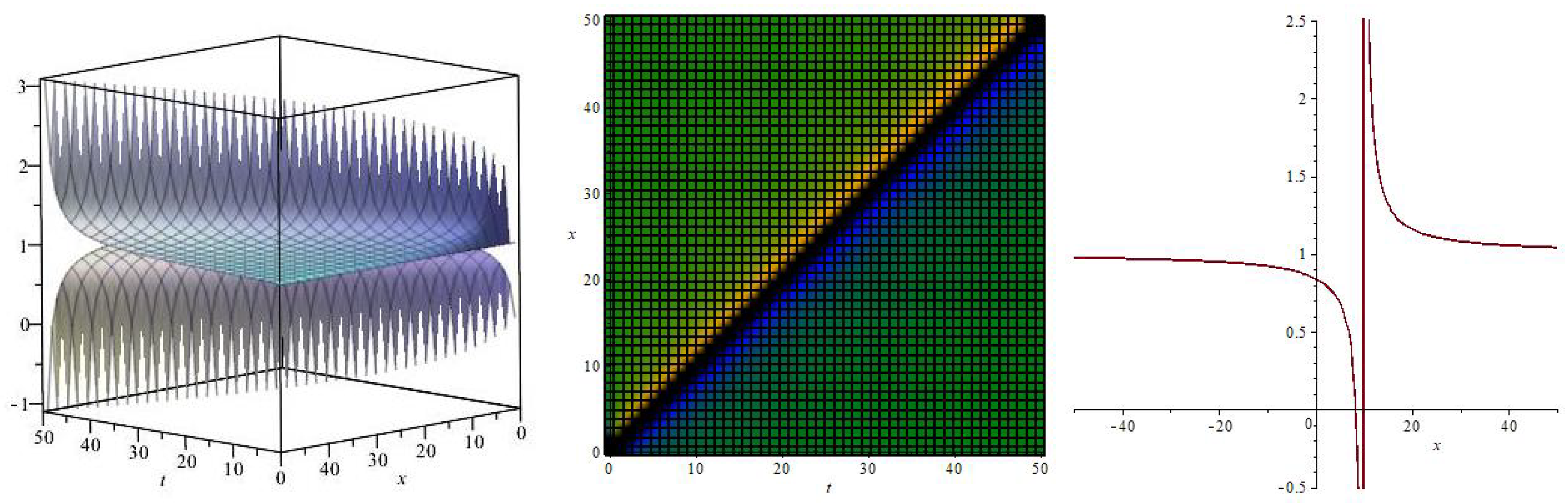
2.3. Invariant Solution under the Symmetry X 6

Finally, we compute the group invariant solution under X 6 . By following the ususal procedure we obtain the group invariant solution
u ( t , x , y , z ) = t 1 5 U ( ξ ) 2 9 t + 2 3 x + 1 3 y + 1 3 z ,
where ξ = t 1 / 5 ( x t ) . Substituting (16) into (3) and simplifying ultimately yields the second-order ODE
ξ U + 2 U = 0 .
Equation (17) can be solved much like Equation (14), which in turn gives the invariant solution of the (3+1)-D gKPe (3) under the group generated by X 6 :
u ( t , x , y , z ) = C 1 + C 2 t 1 / 5 ( x t ) 1
with C 1 , C 2 integration constants. In Figure 3, solution (18) is depicted.
The density plot coupled with the two dimensional profile in Figure 3 depicts a singular soliton-like wave with a singularity in the spatial domain at 0 x 20 .

3. Conserved Quantities of the (3+1)-D gKPe

In this section, we compute the conserved quantities of the (3+1)-D gKPe (3). In our work we use the multiplier approach and the conservation theorem due to Ibragimov to derive the conserved quantities of (3). However, first we provide salient features on both these approaches.

3.1. Multiplier Approach

The multiplier method is one of the most robust and preferred methods for deriving conserved quantities of DEs [4,36,37,38,39,40,41]. This method attempts to mitigate the shortcomings of Noether’s theorem [31], which requires amongst other things, the existence of a variational principle or a Lagrangian before the theorem can be applied. We begin by providing a concise basis of the method.

3.1.1. Preliminaries

Let G be a system of m PDEs of order k, having n independent variables x = ( x 1 , x 2 , , x n ) and m field variables Φ = ( ( Φ 1 , Φ 2 , , Φ m ) ) :
G = ( G 1 ( x , Φ , Φ ( 1 ) , Φ ( 2 ) , , Φ ( k ) ) , , G m ( x , Φ , Φ ( 1 ) , Φ ( 2 ) , , Φ ( k ) ) ) ,
where Φ ( 1 ) , Φ ( 2 ) , , Φ ( k ) denote the derivatives of Φ with respect to the variables x up to the k-th derivative. A local conserved quantity T i ( x , Φ , Φ ( 1 ) , Φ ( 2 ) , , Φ ( l ) ) of system (19) is a continutity equation
D i T i | ε = 0 ,
valid for the solution space ε of system (19).
In general, local nontrivial conserved quantities emanate from the divergence identity
D x 1 T 1 + D x 2 T 2 + + D x n T n = Λ α ( x , Φ , Φ ( 1 ) , Φ ( 2 ) , , Φ ( r ) ) G ( Φ ) .
Here, Λ α ( x , Φ , Φ ( 1 ) , Φ ( 2 ) , , Φ ( r ) ) is a series of conservation law multipiers which are dependent on x, Φ and the derivatives of Φ , up to some arbitrary order r < k . The relationship (21) brings to light the pre-eminent interrelation between conserved quantities T i and multipliers Λ α . A determining condition to derive a set of multipliers Λ α ( x , Φ , Φ ( 1 ) , Φ ( 2 ) , , Φ ( r ) ) for system (19) is that
δ δ Φ α Λ α G = 0 , α = 1 , , m ,
where δ / δ Φ α is the Euler–Lagrange operator given by
δ δ Φ i α = Φ i α + s 1 ( 1 ) s D j 1 D j s Φ i j 1 j 2 j s α , i = 1 , , n , α = 1 , , m .
The condition (22) is requisite and adequate for Λ to be a multiplier. A more rigorous and detailed treatment of the theoretical justification of the multiplier approach including proofs of the formulas utilised in this section can be found in [33].

3.1.2. Application of the Method

In order to determine conserved quantities of Equation (3), we begin by computing the first order multipliers
Λ = Λ ( t , x , u , u x , u y , u z ) ,
by utilising condition (22), that is,
δ δ u Λ E = 0 ,
where
E u t x + u t y + u t z + 3 u x u x y + 3 u x x u y + u x x x y u z z = 0 .
The Euler operator (23) is given by
δ δ u = u D x u x D y u y + D t D x u t x + D t D y u t y + D t D z u t z + D x 2 u x x + D x D y u x y + D z 2 u z z + D x 3 D y u x x x y
and D t , D x , D y and D z are total derivative operators [4]. Expanding (24) and splitting on derivatives of u, we obtain the following system of nine multiplier determining equations:
Λ t y + Λ t z Λ z z = 0 , Λ t u x = 0 , Λ y u x = 0 , Λ z u x = 0 , Λ u x u x = 0 , Λ x = 0 , Λ u = 0 , Λ u y = 0 , Λ u z = 0 .
The solution algorithm of system (25) is simliar to that of obtaining Lie point symmetries. However, with the aid of Gem, a Maple based package [44], this can be expedited. We thus have the multiplier
Λ = C u x
with C an integration constant. The conserved quantities of (3) are obtained via the divergence identity
D t T t + D x T x + D y T y + D z T z = E Λ ,
where T t is a conserved density and T x , T y , T z are spatial fluxes [36]. Thus, after some calculations, we obtain the following conservation law:
T t = 1 2 u x 2 + 1 2 u y u x + 1 2 u z u x , T x = u u x u x y + 2 u x 2 u y + 1 2 u y u x x x 1 2 u x y u x x + 1 2 u x x y u x + 1 2 u u t y + 1 2 u u t z + 1 2 u u x x x y 1 2 u u z z , T y = u u x u x x 1 2 u u t x 1 2 u u x x x x , T z = 1 2 u u t x + 1 2 u u x z 1 2 u z u x .
Since the derivatives of u in the multiplier (26) are of a lower order than both leading derivatives of Equation (3), that is, u t x and u x x x y , the conserved quantities derived here are low-order conservation laws [36].

3.2. Ibragimov’s Approach

We now determine the conservation laws of (3) by applying a theorem due to Ibragimov [42,43]. As in the case of multiplier method, this theorem does not demand availability of a Lagrangian and is established on a concept of an adjoint equation. Thus, it applies to an arbitrary differential equation, irrespective of whether or not it comes from a variational principle.

3.2.1. Preliminaries

The gist of Ibragimov’s method is that every infinitesimal generator is associated with a conserved quantity, notwithstanding the absence of traditional Lagrangians which are envisaged in Noether’s theorem [31]. Below we outline the method in detail.
Consider a system of NLPDEs (19) and its adjoint equations given by
G * ( x , Φ , Ψ , Φ ( 1 ) , Ψ ( 1 ) , Φ ( 2 ) , Ψ ( 2 ) , , Φ ( k ) , Ψ ( k ) ) = δ δ Φ α ( Ψ G β )
where δ / δ Φ α is the Euler–Lagrange operator (23) and m novel field variables Ψ = ( Ψ 1 , , Ψ m ) .
Theorem 1.
Consider a system of m Equations (19). The adjoint system given by (27), inherits the symmetries of the system (19). Namely, if the system (19) admits a point transformation group with a generator X = ξ i / t + η / Φ α , then the adjoint system (27) admits the operator X extended to the variables Ψ α by the formula
Y = ξ i x i + η α Φ α + η * α Ψ α
with appropriately chosen η * α = η * α ( x , Φ , Ψ ) .
The functions ξ i and η α are infinitiesimal generator coefficients dependent on x and Φ . In [43], the coefficients η * α in (28) are given by
η * α = λ β α Ψ β + Ψ α D i ( ξ i ) ,
where λ β α can be computed by utilising the equation
X ( G α ) = λ α β G β .
We can obtain a conserved vector, for instance, for a third-order Lagrangian by applying the formula
C i = ξ i L + W α L Φ i α D j L Φ i j α + D j D k L Φ i j k α + + D j ( W α ) L Φ i j α D k L Φ i j k α + + D j D k ( W α ) L Φ i j k + ,
where L is the Lagrangian of the system G and G * that is defined as
L = Ψ α G α
and W α is the Lie characteristic function given by
W α = η α ξ j Φ j α , α = 1 , , m .
The reader is referred to [42,43] for a more comprehensive discussion of this method.

3.2.2. Application of the Method

To begin, we define the adjoint equation of (3) as [43]
F * = δ δ u v ( u t x + u t y + u t z + 3 u x u x y + 3 u x x u y + u x x x y u z z ) = u D x u x D y u y + D t D x u t x + D t D y u t y + D t D z u t z    + D x 2 u x x + D x D y u x y + D z 2 u z z + D x 3 D y u x x x y v u t x + u t y    + u t z + 3 u x u x y + 3 u x x u y + u x x x y u z z = v t x + v t y + v t z + 6 v x u x y + 3 u x v x y + 3 u y v x x + v x x x y v z z = 0 .
We have introduced a new variable v = v ( t , x , y , z ) . According to [43], the Equation (3) considered together with its adjoint (34) has a Lagrangian L , given by
L = v F = v ( u t x + u t y + u t z + 3 u x u x y + 3 u x x u y + u x x x y u z z ) .
Notice how δ L / δ u = F * and δ L / δ v = F . The Lagrangian (35) is equivalent to the second order Lagrangian
L = v ( u t x + u t y + u t z + 3 u x u x y + 3 u x x u y u z z ) + v x x u x y .
Now, Equation (34) admits all the symmetries (4) and (5) of (3) extended to the new variable v ( t , x , y , z ) . That is, the generators (4) and (5) become
Y = ξ 1 t + ξ 2 x + ξ 3 y + ξ 4 z + η u + η * v
with
η * = η * ( t , x , y , z , u , v ) = λ + D t ( ξ 1 ) + D x ( ξ 2 ) + D y ( ξ 3 ) + D z ( ξ 4 ) v .
The parameter λ is determined by using
X ( F ) = λ F ,
where X is the generator (4) prolonged to all the derivatives in (3), that is,
X = X + ζ x u x + ζ y u y + ζ t x u t x + ζ t y u t y + ζ t z u t z + ζ x x u x x + ζ x y u x y + ζ z z u z z + ζ x x x y u x x x y .
Here X = ξ 1 / t + ξ 2 / x + ξ 3 / y + ξ 4 / z + η / u and ξ 1 , , ξ 4 , and η are functions of ( t , x , y , z , u ) . Furthermore, ζ x , ζ y , ζ t x , ζ t y , ζ t z , ζ x x , ζ x y , ζ z z and ζ x x x y are coefficient functions, each given by the following formulae:
ζ x = D x ( η ) u t D x ( ξ 1 ) u x D x ( ξ 2 ) u y D x ( ξ 3 ) u z D x ( ξ 4 ) , ζ y = D y ( η ) u t D y ( ξ 1 ) u x D y ( ξ 2 ) u y D y ( ξ 3 ) u z D y ( ξ 4 ) , ζ t x = D x ( ζ t ) u t t D x ( ξ 1 ) u t x D x ( ξ 2 ) u t y D x ( ξ 3 ) u t z D x ( ξ 4 ) , ζ t y = D y ( ζ t ) u t t D y ( ξ 1 ) u t x D y ( ξ 2 ) u t y D y ( ξ 3 ) u t z D y ( ξ 4 ) , ζ t z = D z ( ζ t ) u t t D z ( ξ 1 ) u t x D z ( ξ 2 ) u t y D z ( ξ 3 ) u t z D z ( ξ 4 ) , ζ x x = D x ( ζ x ) u x t D x ( ξ 1 ) u x x D x ( ξ 2 ) u x y D x ( ξ 3 ) u x z D x ( ξ 4 ) , ζ x y = D y ( ζ x ) u x t D y ( ξ 1 ) u x x D y ( ξ 2 ) u x y D y ( ξ 3 ) u x z D y ( ξ 4 ) , ζ z z = D z ( ζ x ) u z t D z ( ξ 1 ) u z x D z ( ξ 2 ) u z y D z ( ξ 3 ) u z z D z ( ξ 4 ) , ζ x x x = D x ( ζ x x ) u x x t D x ( ξ 1 ) u x x x D x ( ξ 2 ) u x x y D z ( ξ 3 ) u x x z D x ( ξ 4 ) , ζ x x x y = D y ( ζ x x x ) u x x x t D y ( ξ 1 ) u x x x x D y ( ξ 2 ) u x x x y D y ( ξ 3 ) u x x x z D y ( ξ 4 ) .
See the full expansions of (41) in Appendix A. Now using Equations (3), (39) and (40) we compute the values of the parameter λ corresponding to each of the vector fields in (4) and (5).
Cases X 1 , ⋯, X 4
For the time translation symmetry X 1 , we have ξ 1 = 1 and ξ 2 = ξ 3 = ξ 4 = η = 0 . Thus, it is easy to see that
ζ x = ζ y = ζ t x = ζ t y = ζ t z = ζ x x = ζ x y = ζ z z = ζ x x x y = 0 .
Consequently, we have X 1 ( F ) = 0 F , that is λ = 0 . From (38), we obtain η * = 0 and the new generator (4) retains the form of X 1 , i.e., Y 1 = / t . Since the generator coefficients are all constants, the translation symmetries will retain their form and this leads us to conclude that Y 2 = / x , Y 3 = / y and Y 4 = / z .
Case X 5
Here, we have the generator coefficients ξ 1 = t , ξ 2 = x , ξ 3 = z , ξ 4 = 2 t + z and η = 0 from which we can establish the following:
ζ x = 0 , ζ y = 0 , ζ t x = u t x 2 u x z , ζ t y = u t y 2 u y z , ζ t z = 2 u z z u t x u t y , ζ x x = 0 , ζ x y = 0 , ζ z z = 2 u x z 2 u y z 2 u z z , ζ x x x y = 0 .
Consequently, we can verify that X 5 ( F ) = 0 F , that is, λ = 0 . From (38), we can further establish that η * = 0 . The generator for the adjoint Equation (34) is thus Y 5 = t / t + z / x + z / y + ( 2 t + z ) / z .
Case X 6
The vector field X 6 has the coefficients ξ 1 = 15 t , ξ 2 = 12 t + 3 x , ξ 3 = 9 y 6 z , ξ 4 = 12 t + 3 z and η = 4 x + 4 y 3 u . The reckoning of the coefficient functions (41) yields
ζ x = 4 6 u x , ζ y = 4 12 u y , ζ t x = 21 u t x 12 u x x + 12 u x z , ζ t y = 27 u t y 12 u x y + 12 u y z , ζ t z = 21 u t z 12 u x z + 12 u z z + 6 u t y , ζ x x = 9 u x x , ζ x y = 15 u x y , ζ z z = 9 u z z + 12 u y z , ζ x x x y = 21 u x x x y .
Now, from Equations (39)–(41), we have
X 6 ( F ) = 21 u t x 21 u t y 21 u t z 63 u x u x y 63 u x x u y 21 u x x x y + 21 u z z = 21 ( u t x + u t y + u t z + 3 u x u x y + 3 u x x u y + u x x x y u z z ) = 21 F .
We can thus see that λ = 21 . Consequently,
η * = 21 + D t ( 15 t ) + D x ( 12 t + 3 x ) + D y ( 9 y 6 z ) + D z ( 12 t + 3 z ) v = 7 v .
We now have the vector field:
Y 6 = 15 t t + ( 12 t + 3 x ) x + ( 9 y 6 z ) y + ( 3 z 12 t ) z + ( 4 x + 4 y 3 u ) u 9 v v , corresponding to (34).
Cases X 7 , X 8
Finally, considering the infinite-dimensional vector fields X 7 and X 8 we have, for (34), Y 7 = F ( t ) u and Y 8 = F ( t + z ) u , respectively.
To compute the conservation laws of (3), we utilise the formula [43]
C i = ξ i L + W α L u i α D k L u i k α + D k ( W α ) L u i k α ,
where W α is the Lie characteristic function given by W α = η α ξ j u j α . The reckoning of (42) gives the following conserved quantities:
T 1 = v u z z + 3 v u x u x y + 3 v u y u x x + v u x x x y + 1 2 v z u t + 1 2 v y u t + 1 2 v x u t + 1 2 v u t z + 1 2 v u t y + 1 2 v u t x , X 1 = 3 2 v y u x u t + 3 u y v x u t + 3 2 v u x y u t + 3 4 v x x y u t + 1 2 v t u t 3 2 v u x u t y 1 4 v x x u t y 3 v u y u t x 1 2 v x y u t x + 1 2 v x u t x y + 1 4 v y u t x x 3 4 v u t x x y 1 2 v u t t , Y 1 = 3 2 u x v x u t 3 2 v u x x u t + 1 4 v x x x u t + 1 2 v t u t 3 2 v u x u t x 1 4 v x x u t x + 1 4 v x u t x x 1 4 v u t x x x 1 2 v u t t , Z 1 = v z u t + 1 2 v t u t + v u t z 1 2 v u t t ; T 2 = 1 2 u x z v 1 2 u x y v 1 2 u x x v + 1 2 u x v y + 1 2 u x v z + 1 2 u x v x , X 2 = 3 u x u x y v u z z v + 1 4 u x x x y v + u t z v + u t y v + 1 2 u t x v + 1 2 v t u x + 3 2 u x 2 v y + 3 u x u y v x + 3 4 u x v x x y 1 2 u x x v x y 1 4 v x x u x y + 1 2 v x u x x y + 1 4 u x x x v y , Y 2 = 3 u x x u x v 1 4 u x x x x v 1 2 u t x v + 1 2 v t u x + 3 2 u x 2 v x + 1 4 u x v x x x 1 4 u x x v x x + 1 4 u x x x v x , Z 2 = u x z v 1 2 u t x v + 1 2 v t u x u x v z ;
T 3 = 1 2 u y z v 1 2 u y y v 1 2 u x y v + 1 2 u y v x + 1 2 u y v z + 1 2 u y v y , X 3 = 3 2 u y u x y v 3 2 u x u y y v 3 4 u x x y y v 1 2 u t y v + 1 2 v t u y + 3 u y 2 v x + 3 2 u x u y v y + 3 4 u y v x x y 1 2 u x y v x y + 1 2 v x u x y y 1 4 u y y v x x + 1 4 v y u x x y , Y 3 = u z z v + 3 2 u x u x y v + 3 2 u x x u y v + 3 4 u x x x y v + u t z v + 1 2 u t y v + u t x v + 1 2 v t u y + 3 2 u x u y v x 1 4 v x x u x y + 1 4 v x u x x y + 1 4 u y v x x x , Z 3 = u y z v 1 2 u t y v + 1 2 v t u y u y v z ; T 4 = 1 2 u z v z 1 2 v u z z + 1 2 u z v y 1 2 v u y z + 1 2 u z v x 1 2 v u x z , X 4 = 3 2 u z v y u x 3 2 v u y z u x + 3 u z u y v x 3 v u y u x z + 3 2 v u z u x y 1 2 u x z v x y + 1 2 v x u x y z 1 4 u y z v x x + 1 4 v y u x x z + 3 4 u z v x x y 3 4 v u x x y z + 1 2 u z v t 1 2 v u t z , Y 4 = 3 2 u z u x v x + 1 4 u x x z v x 3 2 v u x u x z 3 2 v u z u x x 1 4 u x z v x x + 1 4 u z v x x x 1 4 v u x x x z + 1 2 u z v t 1 2 v u t z , Z 4 = u z v z + 3 v u x u x y + 3 v u y u x x + v u x x x y + 1 2 u z v t + 1 2 v u t z + v u t y + v u t x ; T 5 = 1 2 v u z + t v z u z + 1 2 z v z u z + t v y u z + 1 2 z v y u z + t v x u z + 1 2 z v x u z 1 2 z v u z z 1 2 v u y + 1 2 z v z u y + 1 2 z u y v y t v u y z z v u y z 1 2 z v u y y 1 2 v u x + 1 2 z v z u x + 1 2 z v y u x + 1 2 z u y v x + 1 2 z u x v x t v u x z z v u x z z v u x y 3 t v u x u x y 1 2 z v u x x 3 t v u y u x x t v u x x x y 1 2 t v z u t 1 2 t v y u t 1 2 t v x u t 1 2 t v u t z 1 2 t v u t y 1 2 t v u t x , X 5 = 3 z v x u y 2 + 3 2 z v y u x u y + 6 t u z v x u y + 3 z u z v x u y + 3 z u x v x u y 6 t v u x z u y 3 z v u x z u y 3 2 z v u x y u y + 3 4 z v x x y u y 3 t v x u t u y + 1 2 z v t u y + 3 t v u t x u y + 3 2 z v y u x 2 v u z z v u z z + 3 t u z v y u x + 3 2 z u z v y u x 3 t v u y z u x 3 2 z v u y z u x 3 2 z v u y y u x + 3 t v u z u x y + 3 2 z v u z u x y + 3 z v u x u x y t u x z v x y 1 2 z u x z v x y 1 2 z u x y v x y + t v x u x y z + 1 2 z v x u x y z + 1 2 z v x u x y y 1 2 z v x y u x x 1 2 t u y z v x x 1 4 z u y z v x x 1 4 z u y y v x x 1 4 z u x y v x x + 1 2 t v y u x x z + 1 4 z v y u x x z + 1 4 z v y u x x y + 1 2 z v x u x x y + 3 2 t u z v x x y + 3 4 z u z v x x y + 3 4 z u x v x x y 3 2 t v u x x y z 3 4 z v u x x y z 3 4 z v u x x y y + 1 4 z v y u x x x + 1 4 z v u x x x y + 1 2 v u t 3 2 t v y u x u t 3 2 t v u x y u t 3 4 t v x x y u t + t u z v t + 1 2 z u z v t + 1 2 z u x v t 1 2 t u t v t t v u t z + 1 2 z v u t z + 1 2 z v u t y + 3 2 t v u x u t y + 1 4 t v x x u t y + 1 2 z v u t x + 1 2 t v x y u t x 1 2 t v x u t x y 1 4 t v y u t x x + 3 4 t v u t x x y + 1 2 t v u t t ,
Y 5 = 3 2 z v x u x 2 + 3 t u z v x u x + 3 2 z u z v x u x + 3 2 z u y v x u x 3 t v u x z u x 3 2 z v u x z u x + 3 2 z v u x y u x 3 z v u x x u x + 1 4 z v x x x u x 3 2 t v x u t u x + 1 2 z v t u x + 3 2 t v u t x u x v u z z v u z z 3 t v u z u x x 3 2 z v u z u x x + 3 2 z v u y u x x 1 2 t u x z v x x 1 4 z u x z v x x 1 4 z u x y v x x 1 4 z u x x v x x + 1 2 t v x u x x z + 1 4 z v x u x x z + 1 4 z v x u x x y + 1 4 z v x u x x x + 1 2 t u z v x x x + 1 4 z u z v x x x + 1 4 z u y v x x x 1 2 t v u x x x z 1 4 z v u x x x z + 3 4 z v u x x x y 1 4 z v u x x x x + 1 2 v u t + 3 2 t v u x x u t 1 4 t v x x x u t + t u z v t + 1 2 z u z v t + 1 2 z u y v t 1 2 t u t v t t v u t z + 1 2 z v u t z + 1 2 z v u t y + 1 2 z v u t x + 1 4 t v x x u t x 1 4 t v x u t x x + 1 4 t v u t x x x + 1 2 t v u t t , Z 5 = 2 t u z v z z u z v z z u y v z z u x v z + t u t v z + v u y + z v u y z + v u x + z v u x z + 6 t v u x u x y + 3 z v u x u x y + 6 t v u y u x x + 3 z v u y u x x + 2 t v u x x x y + z v u x x x y + 1 2 v u t + t u z v t + 1 2 z u z v t + 1 2 z u y v t + 1 2 z u x v t 1 2 t u t v t + 1 2 z v u t z + 2 t v u t y + 1 2 z v u t y + 2 t v u t x + 1 2 z v u t x + 1 2 t v u t t ; T 6 = 3 v u z 9 t u z z v 3 2 z u z z v 3 u y v + 6 t u y z v 9 2 y u y z v + 3 2 z u y z v 9 2 y u y y v + 3 z v u y y 3 u x v 3 2 x u x z v 3 2 z u x z v 6 t u x y v 3 2 x u x y v 9 2 y u x y v + 3 z u x y v + 45 t u x u x y v 6 t u x x v 3 2 x u x x v + 45 t u y u x x v + 15 t u x x x y v + 15 2 t u t z v + 15 2 t u t y v + 15 2 t v u t x + 4 v 2 x v z 2 y v z + 3 2 u v z 6 t u z v z + 3 2 z u z v z + 9 2 y v z u y 3 z v z u y 2 x v y 2 y v y + 3 2 u v y 6 t u z v y + 3 2 z u z v y + 9 2 y u y v y 3 z u y v y + 6 t v z u x + 3 2 x v z u x + 6 t v y u x + 3 2 x v y u x 2 x v x 2 y v x + 3 2 u v x 6 t u z v x + 3 2 z u z v x + 9 2 y u y v x 3 z u y v x + 6 t u x v x + 3 2 x u x v x + 15 2 t v z u t + 15 2 t v y u t + 15 2 t v x u t ,
X 6 = 27 y v x u y 2 18 z v x u y 2 + 12 v u y 36 v u x u y + 27 2 y v y u x u y 9 z v y u x u y 12 x v x u y 12 y v x u y + 9 u v x u y 36 t u z v x u y + 9 z u z v x u y + 36 t u x v x u y + 9 x u x v x u y + 36 t v u x z u y 9 z v u x z u y 27 2 y v u x y u y + 9 z v u x y u y 3 v x x u y + 27 4 y v x x y u y 9 2 z v x x y u y + 45 t v x u t u y + 9 2 y v t u y 3 z v t u y 45 t v u t x u y + 18 t v y u x 2 + 9 2 x v y u x 2 + 6 v u z 12 t v u z z 3 x v u z z 6 x v y u x 6 y v y u x + 9 2 u v y u x 18 t u z v y u x + 9 2 z u z v y u x + 18 t v u y z u x 9 2 z v u y z u x 27 2 y v u y y u x + 9 z v u y y u x 6 x v u x y 6 y v u x y + 9 2 u v u x y 18 t v u z u x y + 9 2 z v u z u x y + 36 t v u x u x y + 9 x v u x u x y + 15 2 v x u x y 3 u x v x y + 6 t u x z v x y 3 2 z u x z v x y 9 2 y u x y v x y + 3 z u x y v x y + 2 v x y 6 t v x u x y z + 3 2 z v x u x y z + 9 2 y v x u x y y 3 z v x u x y y + 9 4 v y u x x 6 t v x y u x x 3 2 x v x y u x x + 3 t u y z v x x 3 4 z u y z v x x 9 4 y u y y v x x + 3 2 z u y y v x x 3 t u x y v x x 3 4 x u x y v x x + v x x 3 t v y u x x z + 3 4 z v y u x x z 27 2 v u x x y + 9 4 y v y u x x y 3 2 z v y u x x y + 6 t v x u x x y + 3 2 x v x u x x y 3 x v x x y 3 y v x x y + 9 4 u v x x y 9 t u z v x x y + 9 4 z u z v x x y + 9 t u x v x x y + 9 4 x u x v x x y + 9 t v u x x y z 9 4 z v u x x y z 27 4 y v u x x y y + 9 2 z v u x x y y + 3 t v y u x x x + 3 4 x v y u x x x + 3 t v u x x x y + 3 4 x v u x x x y 9 v u t + 45 2 t v y u x u t + 45 2 t v u x y u t + 45 4 t v x x y u t 2 x v t 2 y v t + 3 2 u v t 6 t u z v t + 3 2 z u z v t + 6 t u x v t + 3 2 x u x v t + 15 2 t u t v t + 18 t v u t z + 3 x v u t z 3 2 z v u t z + 12 t v u t y + 3 x v u t y 9 2 y v u t y + 3 z v u t y 45 2 t v u x u t y 15 4 t v x x u t y + 6 t v u t x + 3 2 x v u t x 15 2 t v x y u t x + 15 2 t v x u t x y + 15 4 t v y u t x x 45 4 t v u t x x y 15 2 t v u t t ,
Y 6 = 9 v u x 2 + 18 t v x u x 2 + 9 2 x v x u x 2 6 x v x u x 6 y v x u x + 9 2 u v x u x 18 t u z v x u x + 9 2 z u z v x u x + 27 2 y u y v x u x 9 z u y v x u x + 18 t v u x z u x 9 2 z v u x z u x + 27 2 y v u x y u x 9 z v u x y u x 36 t v u x x u x 9 x v u x x u x 3 2 v x x u x + 3 t v x x x u x + 3 4 x v x x x u x + 45 2 t v x u t u x + 6 t v t u x + 3 2 x v t u x 45 2 t v u t x u x + 6 v u z 9 y v u z z + 6 z v u z z + 6 x v u x x + 6 y v u x x 9 2 u v u x x + 18 t v u z u x x 9 2 z v u z u x x + 27 2 y v u y u x x 9 z v u y u x x + 9 4 v x u x x + 3 t u x z v x x 3 4 z u x z v x x 9 4 y u x y v x x + 3 2 z u x y v x x 3 t u x x v x x 3 4 x u x x v x x + v x x 3 t v x u x x z + 3 4 z v x u x x z + 9 4 y v x u x x y 3 2 z v x u x x y 3 v u x x x + 3 t v x u x x x + 3 4 x v x u x x x x v x x x y v x x x + 3 4 u v x x x 3 t u z v x x x + 3 4 z u z v x x x + 9 4 y u y v x x x 3 2 z u y v x x x + 3 t v u x x x z 3 4 z v u x x x z + 27 4 y v u x x x y 9 2 z v u x x x y 3 t v u x x x x 3 4 x v u x x x x 9 v u t 45 2 t v u x x u t + 15 4 t v x x x u t 2 x v t 2 y v t + 3 2 u v t 6 t u z v t + 3 2 z u z v t + 9 2 y u y v t 3 z u y v t + 15 2 t u t v t + 6 t v u t z + 9 y v u t z 15 2 z v u t z + 9 2 y v u t y 3 z v u t y 6 t v u t x 3 2 x v u t x + 9 y v u t x 6 z v u t x 15 4 t v x x u t x + 15 4 t v x u t x x 15 4 t v u t x x x 15 2 t v u t t , Z 6 = 12 v u z + 12 t v z u z 3 z v z u z 6 t v t u z + 3 2 z v t u z + 4 x v z + 4 y v z 3 u v z 6 v u y 9 y v z u y + 6 z v z u y + 9 y v u y z 6 z v u y z 6 v u x 12 t v z u x 3 x v z u x + 12 t v u x z + 3 x v u x z 36 t v u x u x y + 9 z v u x u x y 36 t v u y u x x + 9 z v u y u x x 12 t v u x x x y + 3 z v u x x x y 9 v u t 15 t v z u t 2 x v t 2 y v t + 3 2 u v t + 9 2 y u y v t 3 z u y v t + 6 t u x v t + 3 2 x u x v t + 15 2 t u t v t + 9 t v u t z + 3 2 z v u t z 12 t v u t y 9 2 y v u t y + 6 z v u t y 18 t v u t x 3 2 x v u t x + 3 z v u t x 15 2 t v u t t ; T F 1 = 1 2 F 1 ( t ) v x 1 2 F 1 ( t ) v y 1 2 F 1 ( t ) v z , X F 1 = 3 2 F 1 ( t ) u x y v + 1 2 F 1 v 3 2 F 1 ( t ) u x v y 3 F 1 ( t ) u y v x 3 4 F 1 ( t ) v x x y 1 2 F 1 ( t ) v t , Y F 1 = 3 2 F 1 ( t ) u x x v + 1 2 F 1 v 3 2 F 1 ( t ) u x v x 1 4 F 1 ( t ) v x x x 1 2 F 1 ( t ) v t , Z F 1 = 1 2 F 1 v + F 1 ( t ) v z 1 2 F 1 ( t ) v t ;
T F 2 = 1 2 F 2 v 1 2 v x F 2 ( t + z ) 1 2 v y F 2 ( t + z ) 1 2 v z F 2 ( t + z ) , X F 2 = 3 2 F 2 ( t + z ) u x y v + 1 2 F 2 v 3 2 u x v y F 2 ( t + z ) 3 u y v x F 2 ( t + z ) 3 4 F 2 ( t + z ) v x x y 1 2 v t F 2 ( t + z ) , Y F 2 = 3 2 u x x F 2 ( t + z ) v + 1 2 F 2 v 3 2 u x v x F 2 ( t + z ) 1 4 v x x x F 2 ( t + z ) 1 2 v t F 2 ( t + z ) , Z F 2 = 1 2 F 2 v + v z F 2 ( t + z ) 1 2 v t F 2 ( t + z ) .

4. Concluding Remarks

In this work, we used Lie symmetry methods to obtain analytical solutions of the (3+1)-dimensional generalised KP Equation (3). The first solution contains an elliptic integral of the second kind, an amplitude function, a delta amplitude function and a Jacobi cosine function. It is common knowlegde that these functions degenerate to trigonometric or hyperbolic functions depending on the behaviour of the parameter M 2 . Thus, the solution (13) is to our knowledge the most general solution of (3) that has been obtained to date. Some of the solutions obtained were presented graphically. Furthermore, we obtained logarithmic and rational solutions. Finally, we computed the conserved quantities of Equation (3) using the multiplier method as well as Ibragimov’s conservation theorem. The former method yielded a local low-order conserved quantity, while the later method yielded eight conservation laws with each conserved vector corresponding to an infinitesimal generator.

Author Contributions

Conceptualization, I.S. and C.M.K.; methodology, C.M.K.; software, I.S.; validation, C.M.K.; writing—original draft preparation, I.S.; writing—review and editing, C.M.K. All authors have read and agreed to the published version of the manuscript.

Funding

This research received no external funding.

Acknowledgments

The authors thank North-West University for its continued support and sincerely thank the reviewers for their positive suggestions, which helped to improve the paper enormously.

Conflicts of Interest

The authors declare no conflict of interest.

Appendix A. Prolongation Coefficients: Full Expansions

ζ x = η x + u x η u u t u x ξ u 1 u t ξ x 1 u x 2 ξ u 2 u x ξ x 2 u x u y ξ u 3 u y ξ x 3 u x u z ξ u 4 u z ξ x 4 , ζ y = η y + η u u y u t ξ u 1 u y u t ξ y 1 ξ u 2 u x u y u x ξ y 2 ξ u 4 u y u z u z ξ y 4 u y 2 ξ u 3 u y ξ y 3 , ζ t x = u t u x η u u u t ξ u u 2 u x 2 ξ t u 2 u x 2 2 u t x ξ u 2 u x u t t ξ u 1 u x u t y ξ u 3 u x u t z ξ u 4 u x u t 2 ξ u u 1 u x u y u t ξ u u 3 u x u z u t ξ u u 4 u x u t ξ x u 2 u x + η t u u x u t ξ t u 1 u x u z ξ t u 4 u x ξ t x 2 u x + u t x η u u x x u t ξ u 2 2 u t u t x ξ u 1 u x y u t ξ u 3 u y u t x ξ u 3 u x z u t ξ u 4 u z u t x ξ u 4 u t x ξ x 2 u t t ξ x 1 u t y ξ x 3 u t z ξ x 4 + u t η x u u t 2 ξ x u 1 u y u t ξ x u 3 u z u t ξ x u 4 u x x ξ t 2 u t x ξ t 1 u x y ξ t 3 u x z ξ t 4 + η t x u t ξ t x 1 u y ξ t x 3 u z ξ t x 4 u y ξ t u 3 u x ,
ζ t y = u t η u u u y u t ξ u u 3 u y 2 ξ t u 3 u y 2 u t x ξ u 2 u y u t t ξ u 1 u y 2 u t y ξ u 3 u y u t z ξ u 4 u y u x u t ξ u u 2 u y u t 2 ξ u u 1 u y u z u t ξ u u 4 u y u t ξ y u 3 u y + η t u u y u x ξ t u 2 u y u z ξ t u 4 u y ξ t y 3 u y + u t y η u u x y u t ξ u 2 u x u t y ξ u 2 2 u t u t y ξ u 1 u y y u t ξ u 3 u y z u t ξ u 4 u t ξ t u 1 u y u z u t y ξ u 4 u t x ξ y 2 u t t ξ y 1 u t y ξ y 3 u t z ξ y 4 + u t η y u u x u t ξ y u 2 u t 2 ξ y u 1 u z u t ξ y u 4 u x y ξ t 2 u t y ξ t 1 u y y ξ t 3 u y z ξ t 4 + η t y u x ξ t y 2 u t ξ t y 1 u z ξ t y 4 , ζ t z = u t η u u u z u t ξ u u 4 u z 2 ξ t u 4 u z 2 u t x ξ u 2 u z u t t ξ u 1 u z u t y ξ u 3 u z 2 u t z ξ u 4 u z u x u t ξ u u 2 u z u t 2 ξ u u 1 u z u y u t ξ u u 3 u z u t ξ z u 4 u z + η t u u z u x ξ t u 2 u z u t ξ t u 1 u z u y ξ t u 3 u z ξ t z 4 u z + u t z η u u x z u t ξ u 2 u x u t z ξ u 2 2 u t u t z ξ u 1 u y z u t ξ u 3 u y u t z ξ u 3 u z z u t ξ u 4 u t x ξ z 2 u t t ξ z 1 u t y ξ z 3 u t z ξ z 4 + u t η z u u x u t ξ z u 2 u t 2 ξ z u 1 u y u t ξ z u 3 u x z ξ t 2 u t z ξ t 1 u y z ξ t 3 u z z ξ t 4 + η t z u x ξ t z 2 u t ξ t z 1 u y ξ t z 3 , ζ x x = η u u u x 2 ξ u u 2 u x 3 u t ξ u u 1 u x 2 u y ξ u u 3 u x 2 u z ξ u u 4 u x 2 2 ξ x u 2 u x 2 3 u x x ξ u 2 u x 2 u t x ξ u 1 u x 2 u x y ξ u 3 u x 2 u x z ξ u 4 u x + 2 η x u u x 2 u t ξ x u 1 u x 2 u y ξ x u 3 u x 2 u z ξ x u 4 u x ξ x x 2 u x + u x x η u u x x u t ξ u 1 u y u x x ξ u 3 u z u x x ξ u 4 2 u x x ξ x 2 2 u t x ξ x 1 2 u x y ξ x 3 2 u x z ξ x 4 + η x x u t ξ x x 1 u y ξ x x 3 u z ξ x x 4 , ζ x y = u x η u u u y u x ξ u u 3 u y 2 ξ x u 3 u y 2 u x x ξ u 2 u y u t x ξ u 1 u y 2 u x y ξ u 3 u y u x z ξ u 4 u y u x 2 ξ u u 2 u y u x u t ξ u u 1 u y u z u x ξ u u 4 u y u x ξ y u 3 u y + η x u u y u x ξ x u 2 u y u t ξ x u 1 u y u z ξ x u 4 u y ξ x y 3 u y + u x y η u 2 u x u x y ξ u 2 u x y u t ξ u 1 u x u t y ξ u 1 u y y u x ξ u 3 u y z u x ξ u 4 u z u x y ξ u 4 u x x ξ y 2 u t x ξ y 1 u x y ξ y 3 u x z ξ y 4 + u x η y u u x 2 ξ y u 2 u x u t ξ y u 1 u z u x ξ y u 4 u x y ξ x 2 u t y ξ x 1 u y y ξ x 3 u y z ξ x 4 + η x y u x ξ x y 2 u t ξ x y 1 u z ξ x y 4 , ζ z z = η u u u z 2 ξ u u 4 u z 3 u x ξ u u 2 u z 2 u t ξ u u 1 u z 2 u y ξ u u 3 u z 2 2 ξ z u 4 u z 2 2 u x z ξ u 2 u z 2 u t z ξ u 1 u z 2 u y z ξ u 3 u z 3 u z z ξ u 4 u z + 2 η z u u z 2 u x ξ z u 2 u z 2 u t ξ z u 1 u z 2 u y ξ z u 3 u z ξ z z 4 u z + u z z η u u z z u x ξ u 2 u z z u t ξ u 1 u z z u y ξ u 3 2 u x z ξ z 2 2 u t z ξ z 1 2 u y z ξ z 3 2 u z z ξ z 4 + η z z u x ξ z z 2 u t ξ z z 1 u y ξ z z 3 , ζ x x x y = u y η u u u u u x 3 u y ξ u u u u 2 u x 4 ξ y u u u 2 u x 4 4 u x y ξ u u u 2 u x 3 u t y ξ u u u 1 u x 3 u y y ξ u u u 3 u x 3 u y z ξ u u u 4 u x 3 u y u t ξ u u u u 1 u x 3 u y 2 ξ u u u u 3 u x 3 u z u y ξ u u u u 4 u x 3 + η y u u u u x 3 u t ξ y u u u 1 u x 3 u y ξ y u u u 3 u x 3 u z ξ y u u u 4 u x 3 3 u y ξ x u u u 2 u x 3 3 ξ x y u u 2 u x 3 6 u x x y ξ u u 2 u x 2 3 u t x y ξ u u 1 u x 2 3 u x y y ξ u u 3 u x 2 3 u x y z ξ u u 4 u x 2 + 3 u x y η u u u u x 2 6 u y u x x ξ u u u 2 u x 2 3 u x y u t ξ u u u 1 u x 2 3 u y u t x ξ u u u 1 u x 2 6 u y u x y ξ u u u 3 u x 2 3 u y u x z ξ u u u 4 u x 2 3 u z u x y ξ u u u 4 u x 2 6 u x x ξ y u u 2 u x 2 3 u t x ξ y u u 1 u x 2 3 u x y ξ y u u 3 u x 2 3 u x z ξ y u u 4 u x 2 9 u x y ξ x u u 2 u x 2 3 u t y ξ x u u 1 u x 2 3 u y y ξ x u u 3 u x 2 3 u y z ξ x u u 4 u x 2 + 3 u y η x u u u u x 2 3 u y u t ξ x u u u 1 u x 2 3 u y 2 ξ x u u u 3 u x 2 3 u z u y ξ x u u u 4 u x 2 + 3 η x y u u u x 2 3 u t ξ x y u u 1 u x 2 3 u y ξ x y u u 3 u x 2 3 u z ξ x y u u 4 u x 2 3 u y ξ x x u u 2 u x 2 3 ξ x x y u 2 u x 2 4 u x x x y ξ u 2 u x u x x x x ξ u 2 u x 3 u t x x y ξ u 1 u x u t x x x ξ u 1 u x 3 u x x y y ξ u 3 u x
u x x x y ξ u 3 u x 3 u x x y z ξ u 4 u x u x x x z ξ u 4 u x + 3 u x x y η u u u x 12 u x y u x x ξ u u 2 u x 4 u y u x x x ξ u u 2 u x 3 u x x y u t ξ u u 1 u x 3 u x x u t y ξ u u 1 u x 6 u x y u t x ξ u u 1 u x 3 u y u t x x ξ u u 1 u x 6 u x y 2 ξ u u 3 u x 3 u y y u x x ξ u u 3 u x 6 u y u x x y ξ u u 3 u x 6 u x z u x y ξ u u 4 u x 3 u y z u x x ξ u u 4 u x 3 u y u x x z ξ u u 4 u x 3 u z u x x y ξ u u 4 u x + 3 u y u x x η u u u u x 3 u y u x x u t ξ u u u 1 u x 3 u y 2 u x x ξ u u u 3 u x 3 u z u y u x x ξ u u u 4 u x 4 u x x x ξ y u 2 u x 3 u t x x ξ y u 1 u x 3 u x x y ξ y u 3 u x 3 u x x z ξ y u 4 u x + 3 u x x η y u u u x 3 u x x u t ξ y u u 1 u x 3 u y u x x ξ y u u 3 u x 3 u z u x x ξ y u u 4 u x 9 u x x y ξ x u 2 u x 6 u t x y ξ x u 1 u x 6 u x y y ξ x u 3 u x 6 u x y z ξ x u 4 u x + 6 u x y η x u u u x 9 u y u x x ξ x u u 2 u x 6 u x y u t ξ x u u 1 u x 6 u y u t x ξ x u u 1 u x 12 u y u x y ξ x u u 3 u x 6 u y u x z ξ x u u 4 u x 6 u z u x y ξ x u u 4 u x 9 u x x ξ x y u 2 u x 6 u t x ξ x y u 1 u x 6 u x y ξ x y u 3 u x 6 u x z ξ x y u 4 u x 6 u x y ξ x x u 2 u x 3 u t y ξ x x u 1 u x 3 u y y ξ x x u 3 u x 3 u y z ξ x x u 4 u x + 3 u y η x x u u u x 3 u y u t ξ x x u u 1 u x 3 u y 2 ξ x x u u 3 u x 3 u z u y ξ x x u u 4 u x + 3 η x x y u u x 3 u t ξ x x y u 1 u x 3 u y ξ x x y u 3 u x 3 u z ξ x x y u 4 u x u y ξ x x x u 2 u x ξ x x x y 2 u x + u x x x y η u 6 u x x u x x y ξ u 2 4 u x y u x x x ξ u 2 u x x x y u t ξ u 1 u x x x u t y ξ u 1 3 u x x y u t x ξ u 1 3 u x x u t x y ξ u 1 3 u x y u t x x ξ u 1 3 u x y y u x x ξ u 3 6 u x y u x x y ξ u 3 u y y u x x x ξ u 3 u y u x x x y ξ u 3 3 u x y z u x x ξ u 4 3 u x y u x x z ξ u 4 3 u x z u x x y ξ u 4 u y z u x x x ξ u 4 u z u x x x y ξ u 4 + 3 u x y u x x η u u + u y u x x x η u u 3 u y u x x 2 ξ u u 2 3 u x y u x x u t ξ u u 1 u y u x x x u t ξ u u 1 3 u y u x x u t x ξ u u 1 6 u y u x y u x x ξ u u 3 u y 2 u x x x ξ u u 3 3 u y u x z u x x ξ u u 4 3 u z u x y u x x ξ u u 4 u z u y u x x x ξ u u 4 + u x x x η y u 3 u x x 2 ξ y u 2 u x x x u t ξ y u 1 3 u x x u t x ξ y u 1 3 u x y u x x ξ y u 3 u y u x x x ξ y u 3 3 u x z u x x ξ y u 4 u z u x x x ξ y u 4 3 u x x x y ξ x 2 u x x x x ξ x 2 3 u t x x y ξ x 1 u t x x x ξ x 1 3 u x x y y ξ x 3 u x x x y ξ x 3 3 u x x y z ξ x 4 u x x x z ξ x 4 + 3 u x x y η x u 9 u x y u x x ξ x u 2 3 u y u x x x ξ x u 2 3 u x x y u t ξ x u 1 3 u x x u t y ξ x u 1 6 u x y u t x ξ x u 1 3 u y u t x x ξ x u 1 6 u x y 2 ξ x u 3 3 u y y u x x ξ x u 3 6 u y u x x y ξ x u 3 6 u x z u x y ξ x u 4 3 u y z u x x ξ x u 4 3 u y u x x z ξ x u 4 3 u z u x x y ξ x u 4 + 3 u y u x x η x u u 3 u y u x x u t ξ x u u 1 3 u y 2 u x x ξ x u u 3 3 u z u y u x x ξ x u u 4 3 u x x x ξ x y 2 3 u t x x ξ x y 1 3 u x x y ξ x y 3 3 u x x z ξ x y 4 + 3 u x x η x y u 3 u x x u t ξ x y u 1 3 u y u x x ξ x y u 3 3 u z u x x ξ x y u 4 3 u x x y ξ x x 2 3 u t x y ξ x x 1 3 u x y y ξ x x 3 3 u x y z ξ x x 4 + 3 u x y η x x u 3 u y u x x ξ x x u 2 3 u x y u t ξ x x u 1 3 u y u t x ξ x x u 1 6 u y u x y ξ x x u 3 3 u y u x z ξ x x u 4 3 u z u x y ξ x x u 4 3 u x x ξ x x y 2 3 u t x ξ x x y 1 3 u x y ξ x x y 3 3 u x z ξ x x y 4 u x y ξ x x x 2 u t y ξ x x x 1 u y y ξ x x x 3 u y z ξ x x x 4 + u y η x x x u u y u t ξ x x x u 1 u y 2 ξ x x x u 3 u z u y ξ x x x u 4 + η x x x y u t ξ x x x y 1 u y ξ x x x y 3 u z ξ x x x y 4 .

References

  1. Ovsiannikov, L.V. Group Analysis of Differential Equations; Academic Press: New York, NY, USA, 1982. [Google Scholar]
  2. Ibragimov, N.H. CRC Handbook of Lie Group Analysis of Differential Equations; CRC Press: Boca Raton, FL, USA, 1994; Volume 1. [Google Scholar]
  3. Stephani, H. Differential Equations: Their Solution Using Symmetries; Cambridge University Press: New York, NY, USA, 1989. [Google Scholar]
  4. Olver, P.J. Applications of Lie Groups to Differential Equations, 2nd ed.; Springer: Berlin, Germany, 1993. [Google Scholar]
  5. Hydon, P.E. Symmetry Methods for Differential Equations; Cambridge University Press: Cambridge, UK, 2000. [Google Scholar]
  6. Zhou, Y.; Wang, M.; Li, Z. Application of a homogeneous balance method to exact solutions of nonlinear equations in mathematical physics. Phys. Lett. A 1996, 216, 67–75. [Google Scholar]
  7. Hu, J.; Zhang, H. A new method for finding exact traveling wave solutions to nonlinear partial differential equations. Phys. Lett. A 2001, 286, 175–179. [Google Scholar] [CrossRef]
  8. Hirota, R. The Direct Method in Soliton Theory; Cambridge University Press: Cambridge, UK, 2004. [Google Scholar]
  9. Wang, M.; Li, X.; Zhang, J. The (G/G)-expansion method and travelling wave solutions for linear evolution equations in mathematical physics. Phys. Lett. A 2008, 372, 417–423. [Google Scholar] [CrossRef]
  10. Khalique, C.M.; Moleleki, L.D. A (3+1)-dimensional generalized BKP-Boussinesq equation: Lie group approach. Results Phys. 2019, 13, 102239. [Google Scholar] [CrossRef]
  11. Kudryashov, N.A. One method for finding exact solutions of nonlinear differential equations. Commun. Nonlinear Sci. Numer. Simul. 2012, 17, 2248–2253. [Google Scholar] [CrossRef] [Green Version]
  12. Motsepa, T.; Khalique, C.M. Closed-form solutions and conserved vectors of the (3+1)-dimensional negative-order KdV equation. Adv. Math. Model. Appl. 2020, 5, 7–18. [Google Scholar]
  13. Kudryashov, N.A. Simplest equation method to look for exact solutions of nonlinear differential equations. Chaos Soliton Fract. 2005, 24, 1217–1231. [Google Scholar] [CrossRef] [Green Version]
  14. Simbanefayi, I.; Khalique, C.M. Travelling wave solutions and conservation laws for the Korteweg-de Vries-Benjamin-Bona-Mahony equation. Results Phys. 2018, 8, 57–63. [Google Scholar] [CrossRef]
  15. Zhou, Y.; Wang, M.; Wang, Y. Periodic wave solutions to a coupled KdV equations with variable coefficients. Phys. Lett. A 2003, 308, 31–36. [Google Scholar] [CrossRef]
  16. Zhang, L.; Khalique, C.M. Classification and bifurcation of a class of second-order ODEs and its application to nonlinear PDEs. Discret. Contin. Dynam. Syst. S 2018, 11, 777–790. [Google Scholar] [CrossRef]
  17. Ma, W.X. Comment on the (3+1)-dimensional Kadomtsev–Petviashvili equations. Commun. Nonlinear Sci. Numer. Simul. 2011, 16, 2663–2666. [Google Scholar] [CrossRef]
  18. Kadomtsev, B.B.; Petviashvili, V.I. On the stability of solitary waves in weakly dispersing media. Sov. Phys. Dokl. 1970, 192, 753–756. [Google Scholar]
  19. You, F.; Xia, T.; Chen, D. Decomposition of the generalized KP, cKP and mKP and their exact solutions. Phys. Lett. A 2008, 372, 3184–3194. [Google Scholar] [CrossRef]
  20. Kuznetsov, E.A.; Turitsyn, S.K. Two- and three-dimensional solitons in weakly dispersive media. Zh. Ebp. Teor. Fa. 1982, 82, 1457–1463. [Google Scholar]
  21. Ablowitz, M.J.; Segur, H. On the evolution of packets of water waves. J. Fluid Mech. 1979, 92, 691–715. [Google Scholar] [CrossRef]
  22. Infeld, E.; Rowlands, G. Three-dimensional stability of Korteweg–de Vries waves and solitons II. Acta Phys. Pol. A 1979, 56, 329–332. [Google Scholar]
  23. Senatorski, A.; Infeld, E. Simulations of two-dimensional Kadomtsev–Petviashvili soliton dynamics in three-dimensional space. Phys. Rev. Lett. 1996, 77, 2855–2858. [Google Scholar] [CrossRef]
  24. Alagesan, T.; Uthayakumar, A.; Porsezian, K. Painlevé analysis and Bäcklund transformation for a three-dimensional Kadomtsev–Petviashvili equation. Chaos Soliton Fract. 1997, 8, 893–895. [Google Scholar] [CrossRef]
  25. Xu, G.; Li, Z. Symbolic computation of the Painlevé test for nonlinear partial differential equations using Maple. Comput. Phys. Commun. 2004, 161, 65–75. [Google Scholar] [CrossRef]
  26. Ma, W.X.; Fan, E. Linear superposition principle applying to Hirota bilinear equations. Comput. Math. Appl. 2011, 61, 950–959. [Google Scholar] [CrossRef] [Green Version]
  27. Ma, W.X.; Abdeljabbar, A.; Asaad, M.G. Wronskian and Grammian solutions to a (3+1)-dimensional generalized KP equation. Appl. Math. Comput. 2011, 217, 10016–10023. [Google Scholar] [CrossRef]
  28. Wazwaz, A.M. Multiple-soliton solutions for a (3 +1)-dimensional generalized KP equation, Commun. Nonlinear Sci. Numer. Simul. 2012, 17, 491–495. [Google Scholar] [CrossRef]
  29. Wazwaz, A.M.; El-Tantawy, S.A. A new (3+1)-dimensional generalized Kadomtsev–Petviashvili equation. Nonlinear Dyn. 2016, 84, 1107–1112. [Google Scholar] [CrossRef]
  30. Liu, J.G.; Tian, Y.; Zeng, Z.F. New exact periodic solitary-wave solutions for the new (3+1)-dimensional generalized Kadomtsev–Petviashvili equation in multi-temperature electron plasmas. AIP Adv. 2017, 7, 2158–3226. [Google Scholar] [CrossRef] [Green Version]
  31. Noether, E. Invariante variationsprobleme. Nachr. VD Ges. D. Wiss. Göttingen 1918, 2, 235–257. [Google Scholar]
  32. Bessel-Hagen, E. Uber die Erhaltungsatze der Elektrodynamik. Math. Ann. 1921, 84, 258–276. [Google Scholar] [CrossRef]
  33. Bluman, G.W.; Cheviakov, A.F.; Anco, S.C. Applications of Symmetry Methods to Partial Differential Equations; Springer: New York, NY, USA, 2010. [Google Scholar]
  34. Leveque, R.J. Numerical Methods for Conservation Laws, 2nd ed.; Birkhäuser-Verlag: Basel, Switzerland, 1992. [Google Scholar]
  35. Sarlet, W. Comment on ‘Conservation laws of higher order nonlinear PDEs and the variational conservation laws in the class with mixed derivatives’. J. Phys. A Math. Theor. 2010, 43, 458001. [Google Scholar] [CrossRef]
  36. Anco, S.C. Generalization of Noether’s Theorem in Modern Form to Non-variational Partial Differential Equations. In Recent Progress and Modern Challenges in Applied Mathematics, Modeling and Computational Science; Melnik, R., Makarov, R., Belair, J., Eds.; Fields Institute Communications, Springer: New York, NY, USA, 2017; Volume 79. [Google Scholar]
  37. Johnpillai, A.G.; Khalique, C.M.; Mahomed, F.M. Travelling wave group-invariant solutions and conservation laws for θ-equation. Malays. J. Math. Sci. 2019, 13, 13–29. [Google Scholar]
  38. Motsepa, T.; Abudiab, M.; Khalique, C.M. A Study of an extended generalized (2+1)-dimensional Jaulent-Miodek equation. Int. J. Nonlin. Sci. Numer. Simul. 2018, 19, 391–395. [Google Scholar] [CrossRef]
  39. Khalique, C.M.; Abdallah, S.A. Coupled Burgers equations governing polydispersive sedimentation: A Lie symmetry approach. Results Phys. 2020, 16, 102967. [Google Scholar] [CrossRef]
  40. Bruzón, M.S.; Gandarias, M.L. Traveling wave solutions of the K(m, n) equation with generalized evolution. Math. Meth. Appl. Sci. 2018, 41, 5851–5857. [Google Scholar] [CrossRef]
  41. Khalique, C.M.; Adeyemo, O.D. A study of (3+1)-dimensional generalized Korteweg-de Vries-Zakharov- Kuznetsov equation via Lie symmetry approach. Results Phys. 2020, in press. [Google Scholar]
  42. Ibragimov, N.H. Integrating factors, adjoint equations and Lagrangians. J. Math. Anal. Appl. 2006, 318, 742–757. [Google Scholar] [CrossRef] [Green Version]
  43. Ibragimov, N.H. A new conservation theorem. J. Math. Anal. Appl. 2007, 333, 311–328. [Google Scholar] [CrossRef] [Green Version]
  44. Cheviakov, A.F. Computation of fluxes of conservation laws. J. Eng. Math. 2010, 66, 153–173. [Google Scholar] [CrossRef] [Green Version]
  45. Wazwaz, A.M. Exact soliton and kink solutions for new (3+1)-dimensional nonlinear modified equations of wave propagation. Open Eng. 2017, 7, 169–174. [Google Scholar] [CrossRef]
  46. Baumann, G. Symmetry Analysis of Differential Equations with Mathematica®; Springer: New York, NY, USA, 2000. [Google Scholar]
  47. Gradshteyn, I.S.; Ryzhik, I.M. Table of Integrals, Series, and Products, 7th ed.; Academic Press: New York, NY, USA, 2007. [Google Scholar]
  48. Billingham, J.; King, A.C. Wave Motion; Cambridge University Press: Cambridge, UK, 2000. [Google Scholar]
  49. Korteweg, D.J.; de Vries, G. On the change of form of long waves advancing in a rectangular canal, and on a new type of long stationary waves. Phil Mag. 1895, 39, 422–443. [Google Scholar] [CrossRef]
  50. Drazin, P.G.; Johnson, R.S. Soliton: An Introduction; Cambridge University Press: Cambridge, UK, 1989. [Google Scholar]
Figure 1. Profiles of solution (13).
Mathematics 08 01012 g001
Figure 2. Profiles of solution (15).
Mathematics 08 01012 g002
Figure 3. Profiles of solution (18).
Mathematics 08 01012 g003

