L^p-Solution to the Random Linear Delay Differential Equation with a Stochastic Forcing Term

Abstract

This paper aims at extending a previous contribution dealing with the random autonomous-homogeneous linear differential equation with discrete delay $\tau >0$, by adding a random forcing term $f\left(t\right)$ that varies with time: $x^{\prime }\left(t\right)=ax\left(t\right)+bx(t-\tau )+f\left(t\right)$, $t\ge 0$, with initial condition $x\left(t\right)=g\left(t\right)$, $-\tau \le t\le 0$. The coefficients a and b are assumed to be random variables, while the forcing term $f\left(t\right)$ and the initial condition $g\left(t\right)$ are stochastic processes on their respective time domains. The equation is regarded in the Lebesgue space ${\mathrm{L}}^p$ of random variables with finite p-th moment. The deterministic solution constructed with the method of steps and the method of variation of constants, which involves the delayed exponential function, is proved to be an ${\mathrm{L}}^p$-solution, under certain assumptions on the random data. This proof requires the extension of the deterministic Leibniz’s integral rule for differentiation to the random scenario. Finally, we also prove that, when the delay $\tau$ tends to 0, the random delay equation tends in ${\mathrm{L}}^p$ to a random equation with no delay. Numerical experiments illustrate how our methodology permits determining the main statistics of the solution process, thereby allowing for uncertainty quantification.

1. Introduction

In this paper, we are concerned with random delay differential equations, defined as classical delay differential equations whose inputs (coefficients, forcing term, initial condition, …) are considered as random variables or regular stochastic processes on an underlying complete probability space $(\Omega ,\mathcal{F},\mathbb{P})$, which may take a wide variety of probability distributions, such as Binomial, Poisson, Gamma, Gaussian, etc.

Equations of this kind should not be confused with stochastic differential equations of Itô type, forced by an irregular error term called White noise process (formal derivative of Brownian motion). In contrast to random differential equations, the solutions to stochastic differential equations exhibit nondifferentiable sample-paths. See [1] (pp. 96–98) for a detailed explanation of the difference between random and stochastic differential equations. See [1,2,3,4,5,6], for instance, for applications of random differential equations in engineering, physics, biology, etc. Thus, random differential equations require their own treatment and study: they model smooth random phenomena, with any type of input probability distributions.

From a theoretical viewpoint, random differential equations may be studied in two senses: the sample-path sense or the ${\mathrm{L}}^p$-sense. The former case considers the trajectories of the stochastic processes involved, so that the realizations of the random system correspond to deterministic versions of the problem. The latter case works with the topology of the Lebesgue space $({\mathrm{L}}^p,\parallel ·{\parallel }_p)$ of random variables with finite absolute p-th moment, where the norm ${\parallel ·\parallel }_p$ is defined as: ${\parallel U\parallel }_p={\mathbb{E}\left[\right|U|}^p{]}^{1/p}$ for $1\le p<\infty$ ($\mathbb{E}$ denotes the expectation operator), and ${\parallel U\parallel }_{\infty }=inf\{C\ge 0:|U|\le C\mathrm{almost}\mathrm{surely}\}$ (essential supremum), $U:\Omega \to \mathbb{R}$ being any random variable. The Lebesgue space $({\mathrm{L}}^p,\parallel ·{\parallel }_p)$ has the structure of a Banach space. Continuity, differentiability, Riemann integrability, etc., can be considered in the aforementioned space ${\mathrm{L}}^p$, which gives rise to the random ${\mathrm{L}}^p$-calculus.

In order to fix concepts, given a stochastic process $x\left(t\right)\equiv x(t,\omega )$ on $I\times \Omega$, where $I\subseteq \mathbb{R}$ is an interval (notice that as usual the $\omega$-sample notation might be hidden), we say that x is ${\mathrm{L}}^p$-continuous at $t_0\in I$ if ${lim}_{h\to 0}{\parallel x(t_0+h)-x\left(t_0\right)\parallel }_p=0$. We say that x is ${\mathrm{L}}^p$-differentiable at $t_0\in I$ if ${lim}_{h\to 0}{\parallel \frac{x(t_0+h)-x\left(t_0\right)}{h}-x^{\prime }\left(t_0\right)\parallel }_p=0$, for certain random variable $x^{\prime }\left(t_0\right)$ (called the derivative of x at $t_0$). Finally, if $I=[a,b]$, we say that x is ${\mathrm{L}}^p$-Riemann integrable on $[a,b]$ if there exists a sequence of partitions ${\left\{P_n\right\}}_{n=1}^{\infty }$ with mesh tending to 0, $P_n=\{a=t_0^n<t_1^n<\dots <t_{r_n}^n=b\}$, such that, for any choice of points $s_i^n\in [t_{i-1}^n,t_i^n]$, $i=1,\dots ,r_n$, the limit ${lim}_{n\to \infty }{\sum }_{i=1}^{r_n}x\left(s_i^n\right)(t_i^n-t_{i-1}^n)$ exists in ${\mathrm{L}}^p$. In this case, these Riemann sums have the same limit, which is a random variable and is denoted by ${\int }_a^{b}x\left(t\right)\mathrm{d}t$.

This ${\mathrm{L}}^p$-approach has been widely used in the context of random differential equations with no delay, especially the case $p=2$ which corresponds to the Hilbert space ${\mathrm{L}}^2$ and yields the so-called mean square calculus; see [5,7,8,9,10,11,12,13,14,15]. Only recently, a theoretical probabilistic analysis of random differential equations with discrete constant delay has been addressed in [16,17,18]. In [16], general random delay differential equations in ${\mathrm{L}}^p$ were analyzed, with the goal of extending some of the existing results on random differential equations with no delay from the celebrated book [5]. In [17], we started our study on random delay differential equations with the basic autonomous-homogeneous linear equation, by proving the existence and uniqueness of ${\mathrm{L}}^p$-solution under certain conditions. In [18], the authors studied the same autonomous-homogeneous random linear differential equation with discrete delay as [17], but considered the solution in the sample-path sense and computed its probability density function via the random variable transformation technique, for certain forms of the initial condition process. Other recent contributions for random delay differential equations, but focusing on numerical methods instead, are [19,20,21].

There is still a lack of theoretical analysis for important random delay differential equations. Motivated by this issue, the aim of this contribution is to advance further in the theoretical analysis of relevant random differential equations with discrete delay. In particular, in this paper we extend the recent study performed in [17] for the basic linear equation by adding a stochastic forcing term:

$$\left\{\begin{array}{ccc}{x}^{\prime }(t,\omega )& =& a\left(\omega \right)x(t,\omega )+b\left(\omega \right)x(t-\tau ,\omega )+f(t,\omega ),t\ge 0,\omega \in \Omega ,\hfill \\ x(t,\omega )& =& g(t,\omega ),-\tau \le t\le 0,\omega \in \Omega .\hfill \end{array}\right.$$

(1)

The delay $\tau >0$ is constant. The coefficients a and b are random variables. The forcing term $f\left(t\right)$ and the initial condition $g\left(t\right)$ are stochastic processes on $[0,\infty )$ and $[-\tau ,0]$ respectively, which depend on the outcome $\omega \in \Omega$ of a random experiment which might be sometimes omitted in notation. The term $x\left(t\right)$ represents the differentiable solution stochastic process in a certain probabilistic sense. Formally, according to the deterministic theory [22], we may express the solution process as

$$\begin{array}{ccc}\hfill x(t,\omega )& =\hfill & {\mathrm{e}}^{a\left(\omega \right)(t+\tau )}{\mathrm{e}}_{\tau }^{b_1\left(\omega \right),t}g(-\tau ,\omega )\hfill \\ \hfill & +\hfill & {\int }_{-\tau }^0{\mathrm{e}}^{a\left(\omega \right)(t-s)}{\mathrm{e}}_{\tau }^{b_1\left(\omega \right),t-\tau -s}(g^{\prime }(s,\omega )-a\left(\omega \right)g(s,\omega ))\mathrm{d}s\hfill \\ \hfill & +\hfill & {\int }_0^t{\mathrm{e}}^{a\left(\omega \right)(t-s)}{\mathrm{e}}_{\tau }^{b_1\left(\omega \right),t-\tau -s}f(s,\omega )\mathrm{d}s,\hfill \end{array}$$

(2)

where $b_1={\mathrm{e}}^{-a\tau }b$ and

$${\mathrm{e}}_{\tau }^{c,t}=\left\{\begin{array}{cc}0,\hfill & -\infty <t<-\tau ,\hfill \\ 1,\hfill & -\tau \le t<0,\hfill \\ {\displaystyle 1+c\frac{t}{1!},}\hfill & 0\le t<\tau ,\hfill \\ {\displaystyle 1+c\frac{t}{1!}+c^2\frac{{(t-\tau )}^2}{2!},}\hfill & \tau \le t<2\tau ,\hfill \\ ⋮\hfill & ⋮\hfill \\ {\displaystyle \sum _{k=0}^n{c}^k\frac{{(t-(k-1)\tau )}^k}{k!},}\hfill & (n-1)\tau \le t<n\tau ,\hfill \end{array}\right.$$

is the delayed exponential function [22] (Definition 1), $c,t\in \mathbb{R}$, and $n=\lfloor t/\tau \rfloor +1$ (here $\lfloor ·\rfloor$ denotes the integer part defined by the so-called floor function). This formal solution is obtained with the method of steps and the method of variation of constants.

The primary objective of this paper is to set probabilistic conditions under which $x\left(t\right)$ is an ${\mathrm{L}}^p$-solution to (1). We decompose the original problem (1) as

$$\left\{\begin{array}{ccc}{y}^{\prime }(t,\omega )& =& a\left(\omega \right)y(t,\omega )+b\left(\omega \right)y(t-\tau ,\omega ),t\ge 0,\hfill \\ y(t,\omega )& =& g(t,\omega ),-\tau \le t\le 0,\hfill \end{array}\right.$$

(3)

and

$$\left\{\begin{array}{ccc}{z}^{\prime }(t,\omega )& =& a\left(\omega \right)z(t,\omega )+b\left(\omega \right)z(t-\tau ,\omega )+f(t,\omega ),t\ge 0,\hfill \\ z(t,\omega )& =& 0,-\tau \le t\le 0.\hfill \end{array}\right.$$

(4)

System (3) does not possess a stochastic forcing term, and it was deeply studied in the recent contribution [17]. Under certain assumptions, its ${\mathrm{L}}^p$-solution is expressed as

$$\begin{array}{ccc}\hfill y(t,\omega )& =\hfill & {\mathrm{e}}^{a\left(\omega \right)(t+\tau )}{\mathrm{e}}_{\tau }^{b_1\left(\omega \right),t}g(-\tau ,\omega )\hfill \\ \hfill & +\hfill & {\int }_{-\tau }^0{\mathrm{e}}^{a\left(\omega \right)(t-s)}{\mathrm{e}}_{\tau }^{b_1\left(\omega \right),t-\tau -s}(g^{\prime }(s,\omega )-a\left(\omega \right)g(s,\omega ))\mathrm{d}s,\hfill \end{array}$$

(5)

as a generalization of the deterministic solution to (3) obtained via the method of steps [22] (Theorem 1). Problem (4) is new and requires an analysis in the ${\mathrm{L}}^p$-sense, in order to solve the initial problem (1). Its formal solution is given by

$$z(t,\omega )={\int }_0^t{\mathrm{e}}^{a\left(\omega \right)(t-s)}{\mathrm{e}}_{\tau }^{b_1\left(\omega \right),t-\tau -s}f(s,\omega )\mathrm{d}s,$$

(6)

see [22] (Theorem 2). In order to differentiate (6) in the ${\mathrm{L}}^p$-sense, one requires the extension of the deterministic Leibniz’s integral rule for differentiation to the random scenario. This extension is an important piece of this paper.

In Section 2, we show preliminary results on ${\mathrm{L}}^p$-calculus that are used through the exposition, which correspond to those preliminary results from [17] and the new random Leibniz’s rule for ${\mathrm{L}}^p$-Riemann integration. Auxiliary but novel results to demonstrate the random Leibniz’s integral rule are Fubini’s theorem and a chain rule theorem. In Section 3, we prove in detail that $x\left(t\right)$ defined by (2) is the unique ${\mathrm{L}}^p$-solution to (1), by analyzing problem (4). We also find closed-form expressions for some statistics (expectation and variance) of $x\left(t\right)$ related to its moments. Section 4 deals with the ${\mathrm{L}}^p$-convergence of $x\left(t\right)$ as the delay $\tau$ tends to 0. We then show a numerical example that illustrates the theoretical findings. Finally, Section 5 draws the main conclusions.

In order to complete a fair overview of the existing literature, it must be pointed out that, apart for random delay differential equations (which is the context of this paper), other complementary approaches are stochastic delay differential equations and fuzzy delay differential equations. Stochastic delay differential equations are those in which uncertainty appears due to stochastic processes with irregular sample-paths: the Brownian motion process, Wiener process, Poisson process, etc. A new tool is required to tackle equations of this type, called Itô calculus [23]. Studies on stochastic delay differential equations can be read in [24,25,26,27,28], for example. On the other hand, in fuzzy delay differential equations, uncertainty is driven by fuzzy processes; see [29] for instance. In any of these approaches, the delay might even be considered random; see [30,31].

2. Results on ${\mathrm{L}}^p$-Calculus

In this section, we state the preliminary results on ${\mathrm{L}}^p$-calculus needed for the following sections. Proposition 1 is the chain rule theorem in ${\mathrm{L}}^p$-calculus, which was first proved in [8] (Theorem 3.19) in the setting of mean square calculus ($p=2$). Both Lemma 1 and Lemma 2 provide conditions under which the product of three stochastic processes is ${\mathrm{L}}^p$-continuous or ${\mathrm{L}}^p$-differentiable. Proposition 2 is a result concerning ${\mathrm{L}}^p$-differentiation under the ${\mathrm{L}}^p$-Riemann integral sign, when the interval of integration is fixed. These four results have been already used and stated in the recent contribution [17], and will be required through our forthcoming exposition.

For the sake of completeness, we demonstrate Proposition 2 with an alternative proof to [17], based on Fubini’s theorem for ${\mathrm{L}}^p$-Riemann integration. In the random framework, Fubini’s theorem has not been tackled yet in the recent literature. It states that, if a stochastic process depending on two variables is ${\mathrm{L}}^p$-continuous, then the two iterated ${\mathrm{L}}^p$-Riemann integrals can be interchanged.

We present a new result, Proposition 3, in which we put conditions in order to ${\mathrm{L}}^p$-differentiate an ${\mathrm{L}}^p$-Riemann integral whose interval of integration depends on t. This proposition supposes the extension of the so-called Leibniz’s rule for integration to the random scenario. The proof relies on a new chain rule theorem.

Proposition 1

(Chain rule theorem ([17] Proposition 2.1)). Let $\left\{X\right(t):t\in [a,b\left]\right\}$ be a stochastic process, where $[a,b]$ is any interval in $\mathbb{R}$. Let f be a deterministic $C^1$ function on an open set that contains $X\left(\right[a,b\left]\right)$. Fix $1\le p<\infty$. Let $t\in [a,b]$ be any point such that:

(i)

X is ${\mathrm{L}}^{2p}$-differentiable at t;

(ii)

X is path continuous on $[a,b]$;

(iii)

there exist $r>2p$ and $\delta >0$ such that ${sup}_{s\in [-\delta ,\delta ]}\mathbb{E}\left[\right|f^{\prime }\left(X(t+s)\right){|}^r]<\infty$.

Then $f\circ X$ is ${\mathrm{L}}^p$-differentiable at t and ${(f\circ X)}^{\prime }\left(t\right)=f^{\prime }\left(X\left(t\right)\right)X^{\prime }\left(t\right)$.

Lemma 1

([17] Lemma 2.1). Let $Y_1(t,s)$, $Y_2(t,s)$ and $Y_3(t,s)$ be three stochastic processes and fix $1\le p<\infty$. If $Y_1$ and $Y_2$ are ${\mathrm{L}}^q$-continuous for all $1\le q<\infty$, and $Y_3$ is ${\mathrm{L}}^{p+\eta }$-continuous for certain $\eta >0$, then the product process $Y_1{Y}_2{Y}_3$ is ${\mathrm{L}}^p$-continuous.

On the other hand, if $Y_1$ and $Y_2$ are ${\mathrm{L}}^{\infty }$-continuous, and $Y_3$ is ${\mathrm{L}}^p$-continuous, then the product process $Y_1{Y}_2{Y}_3$ is ${\mathrm{L}}^p$-continuous.

Lemma 2

([17] Lemma 2.2). Let $Y_1\left(t\right)$, $Y_2\left(t\right)$ and $Y_3\left(t\right)$ be three stochastic processes, and $1\le p<\infty$. If $Y_1$ and $Y_2$ are ${\mathrm{L}}^q$-differentiable for all $1\le q<\infty$, and $Y_3$ is ${\mathrm{L}}^{p+\eta }$-differentiable for certain $\eta >0$, then the product process $Y_1{Y}_2{Y}_3$ is ${\mathrm{L}}^p$-differentiable and $\frac{\mathrm{d}}{\mathrm{d}t}\left(Y_1\left(t\right)Y_2\left(t\right)Y_3\left(t\right)\right)=Y_1^{\prime }\left(t\right)Y_2\left(t\right)Y_3\left(t\right)+Y_1\left(t\right)Y_2^{\prime }\left(t\right)Y_3\left(t\right)+Y_1\left(t\right)Y_2\left(t\right)Y_3^{\prime }\left(t\right)$.

Additionally, if $Y_1$ and $Y_2$ are assumed to be ${\mathrm{L}}^{\infty }$-differentiable, and $Y_3$ is ${\mathrm{L}}^p$-differentiable, then $Y_1{Y}_2{Y}_3$ is ${\mathrm{L}}^p$-differentiable, with $\frac{\mathrm{d}}{\mathrm{d}t}\left(Y_1\left(t\right)Y_2\left(t\right)Y_3\left(t\right)\right)=Y_1^{\prime }\left(t\right)Y_2\left(t\right)Y_3\left(t\right)+Y_1\left(t\right)Y_2^{\prime }\left(t\right)Y_3\left(t\right)+Y_1\left(t\right)Y_2\left(t\right)Y_3^{\prime }\left(t\right)$.

Lemma 3

(Fubini’s theorem for iterated ${\mathrm{L}}^p$-Riemann integrals). Let $H(t,s)$ be a process on $[a,b]\times [c,d]$. If H is ${\mathrm{L}}^p$-continuous, then ${\int }_a^b{\int }_c^{d}H(t,s)\mathrm{d}s\mathrm{d}t={\int }_c^d{\int }_a^{b}H(t,s)\mathrm{d}t\mathrm{d}s$, where the integrals are regarded as ${\mathrm{L}}^p$-Riemann integrals.

Proof. 

The proof is a variation of Fubini’s theorem for Itô stochastic integration with respect to the standard Brownian motion ([32] Theorem 2.10.1). The stochastic processes $H(t,s)$, ${\int }_c^{d}H(t,s)\mathrm{d}s$ and ${\int }_a^{b}H(t,s)\mathrm{d}t$ are ${\mathrm{L}}^p$-continuous, so the iterated integrals exist. Let ${\left\{P_n\right\}}_{n=1}^{\infty }$ be a sequence of partitions of $[a,b]$ with mesh tending to 0. Write $P_n=\{a=t_0^n<t_1^n<\cdots <t_n^n=b\}$, and let $r_i^n\in [t_{i-1}^n,t_i^n]$, $1\le i\le n$, $n\ge 1$. Consider the processes $G_n(t,s)={\sum }_{i=1}^{n}H(r_i^n,s){𝟙}_{[t_{i-1}^n,t_i^n]}\left(t\right)$ (here $𝟙$ denotes the characteristic function of a set) and $F_n\left(s\right)={\int }_a^b{G}_n(t,s)\mathrm{d}t={\sum }_{i=1}^{n}H(r_i^n,s)(t_i^n-t_{i-1}^n)$. Notice that, by definition of ${\mathrm{L}}^p$-Riemann integral, ${lim}_{n\to \infty }{F}_n\left(s\right)={\int }_a^{b}H(t,s)\mathrm{d}t$ in ${\mathrm{L}}^p$.

By definition of ${\mathrm{L}}^p$-Riemann integral,

$${\int }_c^d{F}_n\left(s\right)\mathrm{d}s=\sum _{i=1}^n\left({\int }_c^{d}H(r_i^n,s)\mathrm{d}s\right)(t_i^n-t_{i-1}^n)\stackrel{n\to \infty }{⟶}{\int }_a^b{\int }_c^{d}H(t,s)\mathrm{d}s\mathrm{d}t$$

in ${\mathrm{L}}^p$. On the other hand,

$$\begin{array}{ccc}\hfill {\parallel {\int }_c^d{\int }_a^{b}H(t,s)\mathrm{d}t\mathrm{d}s-{\int }_c^d{F}_n\left(s\right)\mathrm{d}s\parallel }_p& =\hfill & {∥{\int }_c^d\left({\int }_a^{b}H(t,s)\mathrm{d}t-F_n\left(s\right)\right)\mathrm{d}s∥}_p\hfill \\ \hfill & \le \hfill & {\int }_c^d{∥{\int }_a^{b}H(t,s)\mathrm{d}t-F_n\left(s\right)∥}_p\mathrm{d}s,\hfill \end{array}$$

where the last inequality is due to a property of ${\mathrm{L}}^p$-integration ([5] p. 102). As $H(t,s)$ and $F_n\left(s\right)$ are ${\mathrm{L}}^p$-bounded on $[a,b]\times [c,d]$ and $[c,d]$, respectively (uniformly on $n\ge 1$), the dominated convergence theorem allows concluding that ${lim}_{n\to \infty }{\int }_c^d{F}_n\left(s\right)\mathrm{d}s={\int }_c^d{\int }_a^{b}H(t,s)\mathrm{d}t\mathrm{d}s$ in ${\mathrm{L}}^p$. □

Proposition 2

(${\mathrm{L}}^p$-differentiation under the ${\mathrm{L}}^p$-Riemann integral sign). Let $F(t,s)$ be a stochastic process on $[a,b]\times [c,d]$. Fix $1\le p<\infty$. Suppose that $F(t,·)$ is ${\mathrm{L}}^p$-continuous on $[c,d]$, for each $t\in [a,b]$, and that there exists the ${\mathrm{L}}^p$-partial derivative $\frac{\partial F}{\partial t}(t,s)$ for all $(t,s)\in [a,b]\times [c,d]$, which is ${\mathrm{L}}^p$-continuous on $[a,b]\times [c,d]$. Let $G\left(t\right)={\int }_c^{d}F(t,s)\mathrm{d}s$ (the integral is understood as an ${\mathrm{L}}^p$-Riemann integral). Then G is ${\mathrm{L}}^p$-differentiable on $[a,b]$ and $G^{\prime }\left(t\right)={\int }_c^d\frac{\partial F}{\partial t}(t,s)\mathrm{d}s$.

Proof. 

We present an alternative and simpler proof to ([17] Proposition 2.2), based on Fubini’s theorem (Lemma 3). Since $\frac{\partial F}{\partial t}$ is ${\mathrm{L}}^p$-continuous, by Barrow’s rule ([5] p. 104) we can write $G\left(t\right)={\int }_c^{d}F(a,s)\mathrm{d}s+{\int }_c^d{\int }_a^t\frac{\partial F}{\partial t}(\tau ,s)\mathrm{d}\tau \mathrm{d}s={\int }_c^{d}F(a,s)\mathrm{d}s+{\int }_a^t{\int }_c^d\frac{\partial F}{\partial t}(\tau ,s)\mathrm{d}s\mathrm{d}\tau$. The stochastic process $\tau \in [a,b]\mapsto {\int }_c^d\frac{\partial F}{\partial t}(\tau ,s)\mathrm{d}s$ is ${\mathrm{L}}^p$-continuous; therefore, $G^{\prime }\left(t\right)={\int }_c^d\frac{\partial F}{\partial t}(t,s)\mathrm{d}s$ in ${\mathrm{L}}^p$, as a consequence of the fundamental theorem for ${\mathrm{L}}^p$-calculus; see ([5] p. 103). □

Lemma 4

(Version of the chain rule theorem). Let $G(t,s)$ be a stochastic process on $[a,b]\times [c,d]$. Let $u:[a,b]\to [c,d]$ be a differentiable deterministic function. Suppose that $G(t,s)$ has ${\mathrm{L}}^p$-partial derivatives, with $\frac{\partial G}{\partial t}(t,s)$ being ${\mathrm{L}}^p$-continuous on $[a,b]\times [c,d]$, and $\frac{\partial G}{\partial s}(t,·)$ being ${\mathrm{L}}^p$-continuous on $[c,d]$, for each $t\in [a,b]$. Then $\frac{\mathrm{d}}{\mathrm{d}t}G(t,u\left(t\right))=\frac{\partial G}{\partial t}(t,u\left(t\right))+u^{\prime }\left(t\right)\frac{\partial G}{\partial s}(t,u\left(t\right))$ in ${\mathrm{L}}^p$.

Proof. 

For $h\ne 0$, by the triangular inequality,

$$\begin{array}{cc}\hfill & {∥\frac{G(t+h,u(t+h\left)\right)-G(t,u(t\left)\right)}{h}-\frac{\partial G}{\partial t}(t,u\left(t\right))-u^{\prime }\left(t\right)\frac{\partial G}{\partial s}(t,u\left(t\right))∥}_p\hfill \\ \hfill \le & \underset{I_1(t,h)}{\underbrace{{∥\frac{G(t+h,u(t+h\left)\right)-G(t,u(t+h\left)\right)}{h}-\frac{\partial G}{\partial t}(t,u\left(t\right))∥}_p}}\hfill \\ \hfill +& \underset{I_2(t,h)}{\underbrace{{∥\frac{G(t,u(t+h\left)\right)-G(t,u(t\left)\right)}{h}-u^{\prime }\left(t\right)\frac{\partial G}{\partial s}(t,u\left(t\right))∥}_p}}.\hfill \end{array}$$

By Barrow’s rule ([5] p. 104) and an inequality from ([5] p. 102),

$$\begin{array}{ccc}\hfill I_1(t,h)& =\hfill & {∥\frac{1}{h}{\int }_t^{t+h}\frac{\partial G}{\partial t}(\tau ,u(t+h))\mathrm{d}\tau -\frac{\partial G}{\partial t}(t,u\left(t\right))∥}_p\hfill \\ \hfill & =\hfill & {∥\frac{1}{h}{\int }_t^{t+h}\left(\frac{\partial G}{\partial t}(\tau ,u(t+h))-\frac{\partial G}{\partial t}(t,u\left(t\right))\right)\mathrm{d}\tau ∥}_p\hfill \\ \hfill & \hfill \le & \frac{1}{\left|h\right|}\left|{\int }_t^{t+h}{∥\frac{\partial G}{\partial t}(\tau ,u(t+h))-\frac{\partial G}{\partial t}(t,u\left(t\right))∥}_p\mathrm{d}\tau \right|.\hfill \end{array}$$

The process $\frac{\partial G}{\partial t}(t,u\left(r\right))$ is ${\mathrm{L}}^p$-uniform continuous on $[a,b]\times [a,b]$; therefore,

$$I_1(t,h)\le \underset{\tau \in [t,t+h]\cup [t+h,t]}{sup}{∥\frac{\partial G}{\partial t}(\tau ,u(t+h))-\frac{\partial G}{\partial t}(t,u\left(t\right))∥}_p\stackrel{h\to 0}{⟶}0.$$

On the other hand, let $Y\left(r\right)=G(t,r)$, for $t\in [a,b]$ fixed. To conclude that ${lim}_{h\to 0}{I}_2(t,h)=0$, we need ${(Y\circ u)}^{\prime }\left(t\right)=Y^{\prime }\left(u\left(t\right)\right)u^{\prime }\left(t\right)$. We have that Y is ${\mathrm{L}}^p$-$C^1\left([c,d]\right)$ and that u is differentiable on $[a,b]$, so the following existing version of the chain rule theorem applies: ([33] Theorem 2.1). □

Remark 1.

Although not needed in the subsequent development, Lemma 4 gives in fact a general multidimensional chain rule theorem for ${\mathrm{L}}^p$-calculus, for the composition of a stochastic process $G(t,s)$ and two deterministic functions $\left(v\right(r),u(r\left)\right)$. This is the generalization of ([33] Theorem 2.1) to several variables. Indeed, let $G(t,s)$ be a stochastic process on an open set $\Lambda \subseteq {\mathbb{R}}^2$, with ${\mathrm{L}}^p$-partial derivatives, $\frac{\partial G}{\partial t}(t,s)$ and $\frac{\partial G}{\partial s}(t,s)$, being ${\mathrm{L}}^p$-continuous on Λ. Let $v,u:[a,b]\to \mathbb{R}$ be two $C^1$ deterministic functions with $\left(v\right(r),u(r\left)\right)\in \Lambda$. Then $\frac{\mathrm{d}}{\mathrm{d}r}G(v\left(r\right),u\left(r\right))=v^{\prime }\left(r\right)\frac{\partial G}{\partial t}(v\left(r\right),u\left(r\right))+u^{\prime }\left(r\right)\frac{\partial G}{\partial s}(v\left(r\right),u\left(r\right))$. For the proof, just define $\overline{G}(t,r)=G(v\left(t\right),r)$. By ([33] Theorem 2.1), $\frac{\partial \overline{G}}{\partial t}(t,r)=v^{\prime }\left(t\right)\frac{\partial G}{\partial t}(v\left(t\right),r)$, which is ${\mathrm{L}}^p$-continuous on $(t,r)$. Additionally, $\frac{\partial \overline{G}}{\partial r}(t,r)=\frac{\partial G}{\partial s}(v\left(t\right),r)$ is ${\mathrm{L}}^p$-continuous. Then $G(v\left(r\right),u\left(r\right))=\overline{G}(r,u\left(r\right))$ can be ${\mathrm{L}}^p$-differentiated at each r, by our Lemma 4: $\frac{\mathrm{d}}{\mathrm{d}r}G(v\left(r\right),u\left(r\right))=\frac{\partial \overline{G}}{\partial t}(r,u\left(r\right))+u^{\prime }\left(r\right)\frac{\partial \overline{G}}{\partial r}(r,u\left(r\right))=v^{\prime }\left(r\right)\frac{\partial G}{\partial t}(v\left(r\right),u\left(r\right))+u^{\prime }\left(r\right)\frac{\partial G}{\partial s}(v\left(r\right),u\left(r\right))$.

Proposition 3

(Random Leibniz’s rule for ${\mathrm{L}}^p$-calculus). Let $F(t,s)$ be a stochastic process on $[a,b]\times [c,d]$. Let $u,v:[a,b]\to [c,d]$ be two differentiable deterministic functions. Suppose that $F(t,·)$ is ${\mathrm{L}}^p$-continuous on $[c,d]$, for each $t\in [a,b]$, and that $\frac{\partial F}{\partial t}(t,s)$ exists in the ${\mathrm{L}}^p$-sense and is ${\mathrm{L}}^p$-continuous on $[a,b]\times [c,d]$. Then $H\left(t\right)={\int }_{u\left(t\right)}^{v\left(t\right)}F(t,s)\mathrm{d}s$ is ${\mathrm{L}}^p$-differentiable and

$$H^{\prime }\left(t\right)=v^{\prime }\left(t\right)F(t,v\left(t\right))-u^{\prime }\left(t\right)F(t,u\left(t\right))+{\int }_{u\left(t\right)}^{v\left(t\right)}\frac{\partial F}{\partial t}(t,s)\mathrm{d}s$$

(the integral is considered as an ${\mathrm{L}}^p$-Riemann integral).

Proof. 

First, notice that $H\left(t\right)$ is well-defined, since $F(t,·)$ is ${\mathrm{L}}^p$-continuous. Decompose $H\left(t\right)$ as $H\left(t\right)={\int }_a^{v\left(t\right)}F(t,s)\mathrm{d}s-{\int }_a^{u\left(t\right)}F(t,s)\mathrm{d}s$. Let $G(t,r)={\int }_a^{r}F(t,s)\mathrm{d}s$, $t\in [a,b]$, $r\in [c,d]$. We have $H\left(t\right)=G(t,v(t\left)\right)-G(t,u(t\left)\right)$.

Let us check the conditions of Lemma 4. By Lemma 2, $\frac{\partial G}{\partial t}(t,r)={\int }_a^r\frac{\partial F}{\partial t}(t,s)\mathrm{d}s$, which is ${\mathrm{L}}^p$-continuous on $[a,b]\times [c,d]$ as a consequence of the ${\mathrm{L}}^p$-continuity of $\frac{\partial F}{\partial t}(t,s)$. On the other hand, $\frac{\partial G}{\partial r}(t,r)=F(t,r)$, by the fundamental theorem of ${\mathrm{L}}^p$-calculus ([5] p. 103), with $\frac{\partial G}{\partial r}(t,·)=F(t,·)$ being ${\mathrm{L}}^p$-continuous. Thus, by Lemma 4,

$$\begin{array}{cc}\hfill H^{\prime }\left(t\right)=& \frac{\partial G}{\partial t}(t,v\left(t\right))+v^{\prime }\left(t\right)\frac{\partial G}{\partial r}(t,v\left(t\right))-\frac{\partial G}{\partial t}(t,u\left(t\right))-u^{\prime }\left(t\right)\frac{\partial G}{\partial r}(t,u\left(t\right))\hfill \\ \hfill =& v^{\prime }\left(t\right)F(t,v\left(t\right))-u^{\prime }\left(t\right)F(t,u\left(t\right))+{\int }_{u\left(t\right)}^{v\left(t\right)}\frac{\partial F}{\partial t}(t,s)\mathrm{d}s.\hfill \end{array}$$

□

Remark 2

(Proposition 3 against another proof of the random Leibniz’s rule). In [10] Proposition 6, a result pointing towards the conclusion of Proposition 3 was stated (in the mean square case $p=2$, with $v\left(t\right)=t$, $u\left(t\right)=0$ and $[c,d]=[a,b]$). However, the proof presented therein is not correct. In the notation therein, the authors proved an inequality of the form

$${\parallel K(t,\Delta t)\parallel }_2\le (t-a)\underset{x\in [a,t]}{max}\parallel K_1{(x,t,\Delta t)\parallel }_2+\underset{x\in [t,t+\Delta t]}{max}{\parallel K_2(x,t,\Delta t)\parallel }_2.$$

The authors justified correctly that $\parallel K_1{(x,t,\Delta t)\parallel }_2\to 0$ and $\parallel K_2{(x,t,\Delta t)\parallel }_2\to 0$ as $\Delta t\to 0$, for each $x\in [a,b]$. However, this fact does not imply

$$\underset{x\in [a,t]}{max}\parallel K_1{(x,t,\Delta t)\parallel }_2\stackrel{\Delta t\to 0}{⟶}0,\underset{x\in [t,t+\Delta t]}{max}{\parallel K_2(x,t,\Delta t)\parallel }_2\stackrel{\Delta t\to 0}{⟶}0,$$

as they stated at the end of their proof. For $K_1$, one has to utilize the dominated convergence theorem. For $K_2$, one should use uniform continuity.

Remark 3

(Random Leibniz’s rule cannot be proved with a mean value theorem). In the deterministic setting, both Proposition 2 and Proposition 3 can be proven with the mean value theorem. However, such proofs do not work in the random scenario, as there is no version of the stochastic mean value theorem. In previous contributions (see [15] Lemma 2.4, Corollary 2.5; [34] Lemma 3.1, Theorem 3.2), there is an incorrect version of it. For instance, if $U\sim \mathrm{Uniform}(0,1)$ and $Y\left(t\right)={𝟙}_{\{t>U\}}\left(t\right)$, $t\in [0,1]$, then Y is mean square continuous on $[0,1]$ (notice that ${\parallel Y\left(t\right)-Y\left(s\right)\parallel }_2^2=|t-s|$). Suppose that there exists $\eta \in [0,1]$ such that ${\int }_0^{1}Y\left(s\right)\mathrm{d}s=Y\left(\eta \right)$ almost surely. Then $Y\left(\eta \right)=1-U$ almost surely. But this is not possible, since $1-U\in (0,1)$ and $Y\left(\eta \right)\in \{0,1\}$. Thus, Y does not satisfy any mean square mean value theorem.

3. ${\mathrm{L}}^p$-Solution to the Random Linear Delay Differential Equation with a Stochastic Forcing Term

In this section we solve (1) in the ${\mathrm{L}}^p$-sense. To do so, we will demonstrate that $x\left(t\right)$ defined by (2) is the unique ${\mathrm{L}}^p$-solution to (1). We will take advantage of the decomposition of problem (1) into its homogeneous part, (3), and its complete part, (4). The formal solution to (3) is given by $y\left(t\right)$ defined as (5), while the formal solution to (4) is given by $z\left(t\right)$ expressed as (6). The previous contribution [17] provides conditions under which $y\left(t\right)$ defined by (5) solves (3) in the ${\mathrm{L}}^p$-sense. Thus, our primary goal will be to find conditions under which $z\left(t\right)$ given by (6) is a true solution to (4) in the ${\mathrm{L}}^p$-sense.

Again, recall that the integrals that appear in the expressions (2), (5) and (6) are ${\mathrm{L}}^p$-Riemann integrals.

The uniqueness (not existence for now) of (1) is proved analogously to ([17] Theorem 3.1), by invoking results from [7] that connect ${\mathrm{L}}^p$-solutions with sample-path solutions, which satisfy analogous properties to deterministic solutions. The precise uniqueness statement is as follows.

Theorem 1

(Uniqueness). The random differential equation problem with delay (1) has at most one ${\mathrm{L}}^p$-solution, for $1\le p<\infty$.

Proof. 

Assume that (1) has an ${\mathrm{L}}^p$-solution. We will prove it is unique. Let $x_1\left(t\right)$ and $x_2\left(t\right)$ be two ${\mathrm{L}}^p$-solutions to (1). Let $u\left(t\right)=x_1\left(t\right)-x_2\left(t\right)$, which satisfies the random differential equation problem with delay

$$\left\{\begin{array}{c}{u}^{\prime }(t,\omega )=a\left(\omega \right)u(t,\omega )+b\left(\omega \right)u(t-\tau ,\omega ),t\ge 0,\hfill \\ u(t,\omega )=0,-\tau \le t\le 0.\hfill \end{array}\right.$$

If $t\in [0,\tau ]$, then $t-\tau \in [-\tau ,0]$; therefore, $u(t-\tau )=0$. Thus, $u\left(t\right)$ satisfies a random differential equation problem with no delay on $[0,\tau ]$:

$$\left\{\begin{array}{c}{u}^{\prime }(t,\omega )=a\left(\omega \right)u(t,\omega ),t\in [0,\tau ],\hfill \\ u(0,\omega )=0.\hfill \end{array}\right.$$

(7)

In [7], it was proved that any ${\mathrm{L}}^p$-solution to a random initial value problem has a product measurable representative which is an absolutely continuous solution in the sample-path sense. Since the sample-path solution to (7) must be 0 (from the deterministic theory), we conclude that $u\left(t\right)=0$ on $[0,\tau ]$, as desired. For the subsequent intervals $[\tau ,2\tau ]$, $[2\tau ,3\tau ]$, etc., the same reasoning applies. □

Now we move on to existence results. First, recall that the random delayed exponential function is the solution to the random linear homogeneous differential equation with pure delay that satisfies the unit initial condition.

Proposition 4

(${\mathrm{L}}^p$-derivative of the random delayed exponential function ([17] Prop 3.1)). Consider the random system with discrete delay

$$\left\{\begin{array}{c}{x}^{\prime }(t,\omega )=c\left(\omega \right)x(t-\tau ,\omega ),t\ge 0,\hfill \\ x(t,\omega )=1,-\tau \le t\le 0,\hfill \end{array}\right.$$

(8)

where $c\left(\omega \right)$ is a random variable.

If c has absolute moments of any order, then ${\mathrm{e}}_{\tau }^{c,t}$ is the unique ${\mathrm{L}}^p$-solution to (8), for all $1\le p<\infty$.

On the other hand, if c is bounded, then ${\mathrm{e}}_{\tau }^{c,t}$ is the unique ${\mathrm{L}}^{\infty }$-solution to (8).

In [17], two results on the existence of solution to (3) were stated and proved. In terms of notation, the moment-generating function of a random variable a is denoted as ${\varphi }_a\left(\zeta \right)=\mathbb{E}\left[{\mathrm{e}}^{a\zeta }\right]$, $\zeta \in \mathbb{R}$.

Theorem 2

(Existence and uniqueness for (3), first version ([17] Theorem 3.2)). Fix $1\le p<\infty$. Suppose that ${\varphi }_a\left(\zeta \right)<\infty$ for all $\zeta \in \mathbb{R}$, b has absolute moments of any order, and g belongs to $C^1\left([-\tau ,0]\right)$ in the ${\mathrm{L}}^{p+\eta }$-sense, for certain $\eta >0$. Then the stochastic process $y\left(t\right)$ defined by (5) is the unique ${\mathrm{L}}^p$-solution to (3).

Theorem 3

(Existence and uniqueness for (3), second version ([17] Theorem 3.4)). Fix $1\le p<\infty$. Suppose that a and b are bounded random variables, and g belongs to $C^1\left([-\tau ,0]\right)$ in the ${\mathrm{L}}^p$-sense. Then the stochastic process $y\left(t\right)$ defined by (5) is the unique ${\mathrm{L}}^p$-solution to (3).

In what follows, we establish two theorems on the existence of a solution to (4); see Theorem 4 and Theorem 5. As a corollary, we will derive the solution to (1); see Theorem 6 and Theorem 7.

Theorem 4

(Existence and uniqueness for (4), first version). Fix $1\le p<\infty$. Suppose that ${\varphi }_a\left(\zeta \right)<\infty$ for all $\zeta \in \mathbb{R}$, b has absolute moments of any order, and f is continuous on $[0,\infty )$ in the ${\mathrm{L}}^{p+\eta }$-sense, for certain $\eta >0$. Then the stochastic process $z\left(t\right)$ defined by (6) is the unique ${\mathrm{L}}^p$-solution to (4).

Proof. 

At the beginning of the proof of ([17] Theorem 3.2), it was proved that $b_1={\mathrm{e}}^{-a\tau }b$ has absolute moments of any order, as a consequence of Cauchy-Schwarz inequality, therefore Proposition 4 tells us that the process ${\mathrm{e}}_{\tau }^{b_1,t}$ is ${\mathrm{L}}^q$-differentiable, for each $1\le q<\infty$, and $\frac{\mathrm{d}}{\mathrm{d}t}{\mathrm{e}}_{\tau }^{b_1,t}=b_1{\mathrm{e}}_{\tau }^{b_1,t-\tau }$. It was also proved that, by the chain rule theorem (Proposition 1), the process ${\mathrm{e}}^{at}$ is ${\mathrm{L}}^q$-differentiable, for each $1\le q<\infty$, and $\frac{\mathrm{d}}{\mathrm{d}t}{\mathrm{e}}^{at}=a{\mathrm{e}}^{at}$. To justify these two assertions on ${\mathrm{e}}_{\tau }^{b_1,t}$ and ${\mathrm{e}}^{at}$, the hypotheses ${\varphi }_a\left(\zeta \right)<\infty$ and b having absolute moments of any order are required.

Fix $0\le s\le t$. Let $Y_1(t,s)={\mathrm{e}}^{a(t-s)}$, $Y_2(t,s)={\mathrm{e}}_{\tau }^{b_1,t-\tau -s}$ and $Y_3\left(s\right)=f\left(s\right)$, according to the notation of Lemma 1. Set the product of the three processes $F(t,s)=Y_1(t,s)Y_2(t,s)Y_3\left(s\right)$, so that our candidate solution process becomes $z\left(t\right)={\int }_0^{t}F(t,s)\mathrm{d}s$. We check the conditions of the random Leibniz’s rule, see Proposition 3, to differentiate $z\left(t\right)$. By the first paragraph of this proof, in which we stated that both ${\mathrm{e}}_{\tau }^{b_1,t}$ and ${\mathrm{e}}^{at}$ are ${\mathrm{L}}^q$-differentiable, for each $1\le q<\infty$, we derive that $Y_1$ and $Y_2$ are ${\mathrm{L}}^q$-continuous on both variables, for all $1\le q<\infty$. Since $Y_3$ is ${\mathrm{L}}^{p+\eta }$-continuous, for certain $\eta >0$ by assumption, we deduce that F is ${\mathrm{L}}^p$-continuous on both variables, as a consequence of Lemma 1.

Fixed s, let $Y_1\left(t\right)={\mathrm{e}}^{a(t-s)}$, $Y_2\left(t\right)={\mathrm{e}}_{\tau }^{b_1,t-\tau -s}$ and $Y_3=f\left(s\right)$. We have that $Y_1$ and $Y_2$ are ${\mathrm{L}}^q$-differentiable, for each $1\le q<\infty$. The random variable $Y_3$ belongs to ${\mathrm{L}}^{p+\eta }$. By Lemma 2, $F(·,s)$ is ${\mathrm{L}}^p$-differentiable at each t, with

$$\frac{\partial F}{\partial t}(t,s)=\left\{a{\mathrm{e}}^{a(t-s)}{\mathrm{e}}_{\tau }^{b_1,t-\tau -s}+{\mathrm{e}}^{a(t-s)}{b}_1{\mathrm{e}}_{\tau }^{b_1,t-2\tau -s}\right\}f\left(s\right).$$

Let us see that $\frac{\partial F}{\partial t}(t,s)$ is ${\mathrm{L}}^p$-continuous at $(t,s)$. Since a has absolute moments of any order (by finiteness of its moment-generating function) and ${\mathrm{e}}^{a(t-s)}$ is ${\mathrm{L}}^q$-continuous at $(t,s)$, for each $1\le q<\infty$, we derive that $a{\mathrm{e}}^{a(t-s)}$ is ${\mathrm{L}}^q$-continuous at each $(t,s)$, for every $1\le q<\infty$, by Hölder’s inequality. Thus, we have that $Y_1(t,s)=a{\mathrm{e}}^{a(t-s)}$ and $Y_2(t,s)={\mathrm{e}}_{\tau }^{b_1,t-\tau -s}$ are ${\mathrm{L}}^q$-continuous at $(t,s)$, for each $1\le q<\infty$, while $Y_3\left(s\right)=f\left(s\right)$ is ${\mathrm{L}}^{p+\eta }$-continuous. By Lemma 1, $a{\mathrm{e}}^{a(t-s)}{\mathrm{e}}_{\tau }^{b_1,t-\tau -s}f\left(s\right)$ is ${\mathrm{L}}^p$-continuous at each $(t,s)$. Analogously, ${\mathrm{e}}^{a(t-s)}{b}_1{\mathrm{e}}_{\tau }^{b_1,t-2\tau -s}f\left(s\right)$ is ${\mathrm{L}}^p$-continuous at $(t,s)$. Therefore, $\frac{\partial F}{\partial t}(t,s)$ is ${\mathrm{L}}^p$-continuous at $(t,s)$. By Proposition 3, the process $z\left(t\right)$ is ${\mathrm{L}}^p$-differentiable and $z^{\prime }\left(t\right)=F(t,t)+{\int }_0^t\frac{\partial F}{\partial t}(t,s)\mathrm{d}s=f\left(t\right)+az\left(t\right)+bz(t-\tau )$ (by definition of $F(t,s)$ in the proof, $F(t,t)={\mathrm{e}}^{a(t-t)}{\mathrm{e}}_{\tau }^{b_1,t-\tau -t}f\left(t\right)={\mathrm{e}}_{\tau }^{b_1,-\tau }f\left(t\right)=f\left(t\right)$, where ${\mathrm{e}}_{\tau }^{b_1,-\tau }=1$ by definition of delayed exponential function), and we are done.

Once the existence of ${\mathrm{L}}^p$-solution has been proved, uniqueness follows from Theorem 1. □

Theorem 5

(Existence and uniqueness for (4), second version). Fix $1\le p<\infty$. Suppose that a and b are bounded random variables, and f is continuous on $[0,\infty )$ in the ${\mathrm{L}}^p$-sense. Then the stochastic process $z\left(t\right)$ defined by (6) is the unique ${\mathrm{L}}^p$-solution to (4).

Proof. 

As was shown in ([17] Theorem 3.4), the process ${\mathrm{e}}_{\tau }^{b_1,t}$ is ${\mathrm{L}}^{\infty }$-differentiable and $\frac{\mathrm{d}}{\mathrm{d}t}{\mathrm{e}}_{\tau }^{b_1,t}=b_1{\mathrm{e}}_{\tau }^{b_1,t-\tau }$, because $b_1=e^{-a\tau }b$ is bounded. Additionally, the process ${\mathrm{e}}^{at}$ is ${\mathrm{L}}^{\infty }$-differentiable and $\frac{\mathrm{d}}{\mathrm{d}t}{\mathrm{e}}^{at}=a{\mathrm{e}}^{at}$, as a consequence of the deterministic mean value theorem and the boundedness of a.

The rest of the proof is completely analogous to the previous Theorem 4, by applying the second part of both Lemma 1 and Lemma 2. □

Theorem 6

(Existence and uniqueness for (1), first version). Fix $1\le p<\infty$. Suppose that ${\varphi }_a\left(\zeta \right)<\infty$ for all $\zeta \in \mathbb{R}$, b has absolute moments of any order, g belongs to $C^1\left([-\tau ,0]\right)$ in the ${\mathrm{L}}^{p+\eta }$-sense and f is continuous on $[0,\infty )$ in the ${\mathrm{L}}^{p+\eta }$-sense, for certain $\eta >0$. Then the stochastic process $x\left(t\right)$ defined by (2) is the unique ${\mathrm{L}}^p$-solution to (1).

Proof. 

This is a consequence of Theorem 2 and Theorem 4, with $x\left(t\right)=y\left(t\right)+z\left(t\right)$. Uniqueness follows from Theorem 1. □

Theorem 7

(Existence and uniqueness for (1), second version). Fix $1\le p<\infty$. Suppose that a and b are bounded random variables, g belongs to $C^1\left([-\tau ,0]\right)$ in the ${\mathrm{L}}^p$-sense and f is continuous on $[0,\infty )$ in the ${\mathrm{L}}^p$-sense. Then the stochastic process $x\left(t\right)$ defined by (2) is the unique ${\mathrm{L}}^p$-solution to (1).

Proof. 

This is a consequence of Theorem 3 and Theorem 5, with $x\left(t\right)=y\left(t\right)+z\left(t\right)$. Uniqueness follows from Theorem 1. □

Remark 4.

As emphasized in ([17] Remark 3.6), the condition of boundedness for a and b in Theorem 7 is necessary if we only assume that $g\in C^1\left([-\tau ,0]\right)$ in the ${\mathrm{L}}^p$-sense. See ([7] Example p. 541), where it is proved that, in order for a random autonomous and homogeneous linear differential equation of first-order to have an ${\mathrm{L}}^p$-solution for every initial condition in ${\mathrm{L}}^p$, one needs the random coefficient to be bounded.

Assume the conditions from Theorem 6 or Theorem 7. From expression (2), it is possible to approximate the statistical moments of $x\left(t\right)$. We focus on its expectation, $\mathbb{E}\left[x\right(t\left)\right]$, and on its variance, $\mathbb{V}\left[x\left(t\right)\right]=\mathbb{E}\left[x{\left(t\right)}^2\right]-{\left(\mathbb{E}\left[x\left(t\right)\right]\right)}^2$. These statistics provide information on the average and the dispersion of $x\left(t\right)$, and they are very useful for uncertainty quantification for $x\left(t\right)$. For ease of notation, denote the stochastic processes

$$F_1(t,\omega )={\mathrm{e}}^{a\left(\omega \right)(t+\tau )}{\mathrm{e}}_{\tau }^{b_1\left(\omega \right),t}g(-\tau ,\omega ),$$

$$F_2(t,s,\omega )={\mathrm{e}}^{a\left(\omega \right)(t-s)}{\mathrm{e}}_{\tau }^{b_1\left(\omega \right),t-\tau -s}(g^{\prime }(s,\omega )-a\left(\omega \right)g(s,\omega )),$$

$$F_3(t,s,\omega )={\mathrm{e}}^{a\left(\omega \right)(t-s)}{\mathrm{e}}_{\tau }^{b_1\left(\omega \right),t-\tau -s}f(s,\omega ).$$

Due to the linearity of the expectation and its interchangeability with the ${\mathrm{L}}^1$-Riemann integral ([5] p. 104), if $p\ge 1$,

$$\mathbb{E}\left[x\left(t\right)\right]=\mathbb{E}\left[F_1\left(t\right)\right]+{\int }_{-\tau }^0\mathbb{E}\left[F_2(t,s)\right]\mathrm{d}s+{\int }_0^t\mathbb{E}\left[F_3(t,s)\right]\mathrm{d}s.$$

(9)

To compute $\mathbb{V}\left[x\right(t\left)\right]$ when $p\ge 2$, we start by

$$\begin{array}{cc}\hfill x{\left(t\right)}^2=& F_1{\left(t\right)}^2+{\int }_{-\tau }^0{\int }_{-\tau }^0{F}_2(t,s_1)F_2(t,s_2)\mathrm{d}{s}_2\mathrm{d}{s}_1\hfill \\ \hfill +& {\int }_0^t{\int }_0^t{F}_3(t,s_1)F_3(t,s_2)\mathrm{d}{s}_2\mathrm{d}{s}_1+2{\int }_{-\tau }^0{F}_1\left(t\right)F_2(t,s)\mathrm{d}s\hfill \\ \hfill +& 2{\int }_0^t{F}_1\left(t\right)F_3(t,s)\mathrm{d}s+2{\int }_{-\tau }^0{\int }_0^t{F}_2(t,s_1)F_3(t,s_2)\mathrm{d}{s}_2\mathrm{d}{s}_1.\hfill \end{array}$$

Each of these integrals has to be considered in ${\mathrm{L}}^{p/2}$; see ([35] Remark 2). This is due to the loss of integrability of the product, by Hölder’s inequality. By applying expectations,

$$\begin{array}{cc}\hfill \mathbb{E}\left[x{\left(t\right)}^2\right]=& \mathbb{E}\left[F_1{\left(t\right)}^2\right]+{\int }_{-\tau }^0{\int }_{-\tau }^0\mathbb{E}\left[F_2(t,s_1)F_2(t,s_2)\right]\mathrm{d}{s}_2\mathrm{d}{s}_1\hfill \\ \hfill +& {\int }_0^t{\int }_0^t\mathbb{E}\left[F_3(t,s_1)F_3(t,s_2)\right]\mathrm{d}{s}_2\mathrm{d}{s}_1+2{\int }_{-\tau }^0\mathbb{E}\left[F_1\left(t\right)F_2(t,s)\right]\mathrm{d}s\hfill \\ \hfill +& 2{\int }_0^t\mathbb{E}\left[F_1\left(t\right)F_3(t,s)\right]\mathrm{d}s+2{\int }_{-\tau }^0{\int }_0^t\mathbb{E}\left[F_2(t,s_1)F_3(t,s_2)\right]\mathrm{d}{s}_2\mathrm{d}{s}_1.\hfill \end{array}$$

(10)

As a consequence, one derives an expression for $\mathbb{V}\left[x\right(t\left)\right]$, by utilizing the relation $\mathbb{V}\left[x\left(t\right)\right]=\mathbb{E}\left[x{\left(t\right)}^2\right]-{\left(\mathbb{E}\left[x\left(t\right)\right]\right)}^2$. Other statistics related to moments could be derived in a similar fashion.

In Example 1, we will show how useful these expressions are to determine $\mathbb{E}\left[x\right(t\left)\right]$ and $\mathbb{V}\left[x\right(t\left)\right]$ in practice. Our procedure is an alternative to the usual techniques for uncertainty quantification: Monte Carlo simulation, generalized polynomial chaos (gPC) expansions, etc. [1,2].

4. ${\mathrm{L}}^p$-Convergence to a Random Complete Linear Differential Equation When the Delay Tends to 0

Given a discrete delay $\tau >0$, we denote the ${\mathrm{L}}^p$-solution (2) to (1) by $x_{\tau }\left(t\right)$. We denote the ${\mathrm{L}}^p$-solutions (5) and (6) to (3) and (4) by $y_{\tau }\left(t\right)$ and $z_{\tau }\left(t\right)$, respectively, so that $x_{\tau }\left(t\right)=y_{\tau }\left(t\right)+z_{\tau }\left(t\right)$. Thus, we are making the dependence on the delay $\tau$ explicit. If we put $\tau =0$ into (1), (3) and (4), we obtain random linear differential equations with no delay:

$$\left\{\begin{array}{c}{x}_0^{\prime }(t,\omega )=(a\left(\omega \right)+b\left(\omega \right))x_0(t,\omega )+f(t,\omega ),t\ge 0,\hfill \\ x_0(0,\omega )=g(0,\omega ),\hfill \end{array}\right.$$

(11)

$$\left\{\begin{array}{c}{y}_0^{\prime }(t,\omega )=(a\left(\omega \right)+b\left(\omega \right))y_0(t,\omega ),t\ge 0,\hfill \\ y_0(0,\omega )=g(0,\omega ),\hfill \end{array}\right.$$

(12)

$$\left\{\begin{array}{c}{z}_0^{\prime }(t,\omega )=(a\left(\omega \right)+b\left(\omega \right))z_0(t,\omega )+f(t,\omega ),t\ge 0,\hfill \\ z_0(0,\omega )=0,\hfill \end{array}\right.$$

(13)

respectively. The following results establish conditions under which (11), (12) and (13) have ${\mathrm{L}}^p$-solutions.

Theorem 8

([17] Corollary 4.1). Fix $1\le p<\infty$. If ${\varphi }_a\left(\zeta \right)<\infty$ and ${\varphi }_b\left(\zeta \right)<\infty$ for all $\zeta \in \mathbb{R}$, and $g\left(0\right)\in {\mathrm{L}}^{p+\eta }$ for certain $\eta >0$, then the stochastic process $y_0\left(t\right)=g\left(0\right){\mathrm{e}}^{(a+b)t}$ is the unique ${\mathrm{L}}^p$-solution to (12).

On the other hand, if a and b are bounded random variables and $g\left(0\right)\in {\mathrm{L}}^p$, then the stochastic process $y_0\left(t\right)=g\left(0\right){\mathrm{e}}^{(a+b)t}$ is the unique ${\mathrm{L}}^p$-solution to (12).

Theorem 9.

Fix $1\le p<\infty$. If ${\varphi }_a\left(\zeta \right)<\infty$ and ${\varphi }_b\left(\zeta \right)<\infty$ for all $\zeta \in \mathbb{R}$, and f is continuous on $[0,\infty )$ in the ${\mathrm{L}}^{p+\eta }$-sense for certain $\eta >0$, then the stochastic process $z_0\left(t\right)={\int }_0^t{\mathrm{e}}^{(a+b)(t-s)}f\left(s\right)\mathrm{d}s$ is the unique ${\mathrm{L}}^p$-solution to (13).

On the other hand, if a and b are bounded random variables and f is continuous on $[0,\infty )$ in the ${\mathrm{L}}^p$-sense, then the stochastic process $z_0\left(t\right)={\int }_0^t{\mathrm{e}}^{(a+b)(t-s)}f\left(s\right)\mathrm{d}s$ is the unique ${\mathrm{L}}^p$-solution to (13).

Proof. 

Take the first set of assumptions. Let $F(t,s)={\mathrm{e}}^{(a+b)(t-s)}f\left(s\right)$ be the process inside the integral sign. Since ${\varphi }_a<\infty$ and ${\varphi }_b<\infty$, the chain rule theorem (Proposition 1) allows differentiating ${\mathrm{e}}^{(a+b)t}$ in ${\mathrm{L}}^q$, for each $1\le q<\infty$. In particular, ${\mathrm{e}}^{(a+b)(t-s)}$ is ${\mathrm{L}}^q$-continuous at $(t,s)$, for $1\le q<\infty$. As f is continuous on $[0,\infty )$ in the ${\mathrm{L}}^{p+\eta }$-sense, we derive that F is ${\mathrm{L}}^p$-continuous at $(t,s)$. It also exists $\frac{\partial F}{\partial t}(t,s)=(a+b){\mathrm{e}}^{(a+b)(t-s)}f\left(s\right)$ in ${\mathrm{L}}^p$. Since $a+b$ has absolute moments of any order, $(a+b){\mathrm{e}}^{(a+b)(t-s)}$ is ${\mathrm{L}}^q$-continuous at $(t,s)$, for $1\le q<\infty$. Then $\frac{\partial F}{\partial t}$ is ${\mathrm{L}}^p$-continuous at $(t,s)$. By Proposition 3, $z_0$ is ${\mathrm{L}}^p$-differentiable and $z_0^{\prime }\left(t\right)=F(t,t)+{\int }_0^t\frac{\partial F}{\partial t}(t,s)\mathrm{d}s=f\left(t\right)+(a+b)z_0\left(t\right)$, and we are done.

Suppose that a and b are bounded random variables and f is continuous on $[0,\infty )$ in the ${\mathrm{L}}^p$-sense. If a and b are bounded, then ${\mathrm{e}}^{(a+b)t}$ is ${\mathrm{L}}^{\infty }$-differentiable (this is because of an application of the deterministic mean value theorem; see ([17] Theorem 3.4)). Then an analogous proof to the previous paragraph works in this case, by only assuming that f is continuous on $[0,\infty )$ in the ${\mathrm{L}}^p$-sense. □

Theorem 10.

Fix $1\le p<\infty$. If ${\varphi }_a\left(\zeta \right)<\infty$ and ${\varphi }_b\left(\zeta \right)<\infty$ for all $\zeta \in \mathbb{R}$, $g\left(0\right)\in {\mathrm{L}}^{p+\eta }$, and f is continuous on $[0,\infty )$ in the ${\mathrm{L}}^{p+\eta }$-sense for certain $\eta >0$, then the stochastic process $x_0\left(t\right)=g\left(0\right){\mathrm{e}}^{(a+b)t}+{\int }_0^t{\mathrm{e}}^{(a+b)(t-s)}f\left(s\right)\mathrm{d}s$ is the unique ${\mathrm{L}}^p$-solution to (11).

On the other hand, if a and b are bounded random variables, $g\left(0\right)\in {\mathrm{L}}^p$, and f is continuous on $[0,\infty )$ in the ${\mathrm{L}}^p$-sense, then the stochastic process $x_0\left(t\right)=g\left(0\right){\mathrm{e}}^{(a+b)t}+{\int }_0^t{\mathrm{e}}^{(a+b)(t-s)}f\left(s\right)\mathrm{d}s$ is the unique ${\mathrm{L}}^p$-solution to (11).

Proof. 

It is a consequence of Theorem 8 and Theorem 9 with $x_0\left(t\right)=y_0\left(t\right)+z_0\left(t\right)$. □

Our goal is to establish conditions under which ${lim}_{\tau \to 0}{x}_{\tau }\left(t\right)=x_0\left(t\right)$ in ${\mathrm{L}}^p$, for each $t\ge 0$. To do so, we will utilize ${lim}_{\tau \to 0}{y}_{\tau }\left(t\right)=y_0\left(t\right)$ and ${lim}_{\tau \to 0}{z}_{\tau }\left(t\right)=z_0\left(t\right)$.

The first limit, ${lim}_{\tau \to 0}{y}_{\tau }\left(t\right)=y_0\left(t\right)$, was demonstrated in ([17] Theorem 4.5), by using inequalities for the deterministic and random delayed exponential function ([36] Theorem A.3), ([17] Lemma 4.2, Lemma 4.3, Lemma 4.4).

Theorem 11

([17] Theorem 4.5). Fix $1\le p<\infty$. Let a and b be bounded random variables and let g be a stochastic process that belongs to $C^1\left([-\tau ,0]\right)$ in the ${\mathrm{L}}^p$-sense. Then, ${lim}_{\tau \to 0}{y}_{\tau }\left(t\right)=y_0\left(t\right)$ in ${\mathrm{L}}^p$, uniformly on $[0,T]$, for each $T>0$.

Next we prove the convergence ${lim}_{\tau \to 0}{z}_{\tau }\left(t\right)=z_0\left(t\right)$. As a corollary, we will be able to derive ${lim}_{\tau \to 0}{x}_{\tau }\left(t\right)=x_0\left(t\right)$.

Theorem 12.

Fix $1\le p<\infty$. Let a and b be bounded random variables and let f be a continuous stochastic process on $[0,\infty )$ in the ${\mathrm{L}}^p$-sense. Then, ${lim}_{\tau \to 0}{z}_{\tau }\left(t\right)=z_0\left(t\right)$ in ${\mathrm{L}}^p$, uniformly on $[0,T]$, for each $T>0$.

Proof. 

Notice that $z_{\tau }\left(t\right)$ defined by (6) (see the first paragraph of this section) exists by Theorem 5, which used the boundedness of a and b and the ${\mathrm{L}}^p$-continuity of f on $[0,\infty )$. Analogously, $z_0\left(t\right)$ exists by Theorem 9.

Fix $t\in [0,T]$. We bound

$$\begin{array}{cc}\hfill \parallel z_{\tau }\left(t\right)-z_0{\left(t\right)\parallel }_p\le & {\int }_0^t{∥{\mathrm{e}}^{a(t-s)}f\left(s\right)\left({\mathrm{e}}_{\tau }^{b_1,t-\tau -s}-{\mathrm{e}}^{b(t-s)}\right)∥}_p\mathrm{d}s\hfill \\ \hfill \le & {\int }_0^t{∥{\mathrm{e}}^{a(t-s)}∥}_{\infty }{\parallel f\left(s\right)\parallel }_p{∥{\mathrm{e}}_{\tau }^{b_1,t-\tau -s}-{\mathrm{e}}^{b(t-s)}∥}_{\infty }\mathrm{d}s.\hfill \end{array}$$

We have $\parallel e^{a(t-s)}{\parallel }_{\infty }\le {\mathrm{e}}^{{\parallel a\parallel }_{\infty }T}$ and ${\parallel f\left(s\right)\parallel }_p\le C_f={max}_{s\in [0,T]}{\parallel f\left(s\right)\parallel }_p$. These bounds yield

$$\parallel z_{\tau }\left(t\right)-z_0{\left(t\right)\parallel }_p\le C_f{\mathrm{e}}^{{\parallel a\parallel }_{\infty }T}{\int }_0^t{∥{\mathrm{e}}_{\tau }^{b_1,t-\tau -s}-{\mathrm{e}}^{b(t-s)}∥}_{\infty }\mathrm{d}s.$$

(14)

Let k be a number such that $k\ge \parallel b_1{\parallel }_{\infty }={\parallel {\mathrm{e}}^{a\tau }b\parallel }_{\infty }$, for all $\tau \in (0,1]$. By ([17] Lemma 4.3),

$${∥{\mathrm{e}}_{\tau }^{b_1,t-\tau -s}-{\mathrm{e}}^{b_1(t-s)}∥}_{\infty }\le C_{T,k}·\tau ,$$

(15)

for $t\in [0,T]$, $0\le s\le t$ and $\tau \in (0,1]$. On the other hand, by the deterministic mean value theorem (applied for each outcome $\omega$),

$$\begin{array}{cc}\hfill {\mathrm{e}}^{b_1(t-s)}-{\mathrm{e}}^{b(t-s)}=& {\mathrm{e}}^{{\mathrm{e}}^{-a\tau }b(t-s)}-{\mathrm{e}}^{b(t-s)}\hfill \\ \hfill =& b(t-s){\mathrm{e}}^{{\xi }_{\tau ,\omega }b(t-s)}({\mathrm{e}}^{-a\tau }-1),\hfill \end{array}$$

where ${\xi }_{\tau ,\omega }\in (1,{\mathrm{e}}^{-a\tau })\cup ({\mathrm{e}}^{-a\tau },1)$. In particular, $|{\xi }_{\tau ,\omega }|\le 1+{\mathrm{e}}^{{\parallel a\parallel }_{\infty }}$. We apply again the deterministic mean value theorem to ${\mathrm{e}}^{-a\tau }-1$:

$${\mathrm{e}}^{-a\tau }-1={\mathrm{e}}^{{\overline{\xi }}_{\tau ,\omega }}(-a\tau ),$$

where ${\overline{\xi }}_{\tau ,\omega }\in (-a\tau ,0)\cup (0,-a\tau )$. In particular,

$$\parallel {\mathrm{e}}^{-a\tau }{-1\parallel }_{\infty }\le {\mathrm{e}}^{{\parallel a\parallel }_{\infty }}{\parallel a\parallel }_{\infty }\tau .$$

As a consequence,

$$\parallel {\mathrm{e}}^{b_1(t-s)}-{\mathrm{e}}^{b(t-s)}{\parallel }_{\infty }\le \underset{{\overline{C}}_{{T,\parallel a\parallel }_{\infty },{\parallel b\parallel }_{\infty }}}{\underbrace{{\parallel b\parallel }_{\infty }T{\mathrm{e}}^{(1+{\mathrm{e}}^{{\parallel a\parallel }_{\infty }}){\parallel b\parallel }_{\infty }T}{\mathrm{e}}^{{\parallel a\parallel }_{\infty }}{\parallel a\parallel }_{\infty }}}\tau .$$

(16)

By combining (15) and (16) and by the triangular inequality,

$$\begin{array}{cc}\hfill {∥{\mathrm{e}}_{\tau }^{b_1,t-\tau -s}-{\mathrm{e}}^{b(t-s)}∥}_{\infty }\le & {∥{\mathrm{e}}_{\tau }^{b_1,t-\tau -s}-{\mathrm{e}}^{b_1(t-s)}∥}_{\infty }\hfill \\ \hfill +& {∥{\mathrm{e}}^{b_1(t-s)}-{\mathrm{e}}^{b(t-s)}∥}_{\infty }\le \left(C_{T,k}+{\overline{C}}_{{T,\parallel a\parallel }_{\infty },{\parallel b\parallel }_{\infty }}\right)\tau .\hfill \end{array}$$

Substituting this inequality into (14),

$$\parallel z_{\tau }\left(t\right)-z_0{\left(t\right)\parallel }_p\le C_f{\mathrm{e}}^{{\parallel a\parallel }_{\infty }T}\left(C_{T,k}+{\overline{C}}_{{T,\parallel a\parallel }_{\infty },{\parallel b\parallel }_{\infty }}\right)\tau \stackrel{\tau \to 0}{⟶}0,$$

uniformly on $[0,T]$. □

Theorem 13.

Fix $1\le p<\infty$. Let a and b be bounded random variables, let g be a stochastic process that belongs to $C^1\left([-\tau ,0]\right)$ in the ${\mathrm{L}}^p$-sense, and let f be a continuous stochastic process on $[0,\infty )$ in the ${\mathrm{L}}^p$-sense. Then, ${lim}_{\tau \to 0}{x}_{\tau }\left(t\right)=x_0\left(t\right)$ in ${\mathrm{L}}^p$, uniformly on $[0,T]$, for each $T>0$.

Proof. 

This is a consequence of Theorem 11 and Theorem 12, with $x_{\tau }\left(t\right)=y_{\tau }\left(t\right)+z_{\tau }\left(t\right)$ and $x_0\left(t\right)=y_0\left(t\right)+z_0\left(t\right)$. □

Example 1.

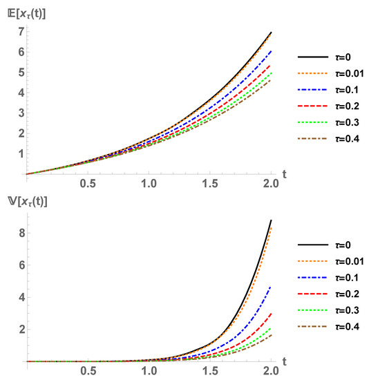
This is a test example, with arbitrary distributions, to show how (9) and (10) may be employed to compute the expectation and the variance of the stochastic solution. Theoretical results are also illustrated. Let $a\sim \mathrm{Beta}(2,3)$ and $b\sim \mathrm{Uniform}(0.2,1)$. Define $g(t,\omega )=sin(sin\left(d\left(\omega \right)t^2\right))$ and $f(t,\omega )=cos\left(te{\left(\omega \right)}^2\right)$, where d and e are random variables with $d\sim \mathrm{Triangular}(1,1.15,1.3)$ and $e\sim \mathrm{Uniform}(0.1,0.2)$. By using the chain rule theorem, Proposition 1, it is easy to prove that both g and f are $C^{\infty }$ in the ${\mathrm{L}}^p$-sense, $1\le p<\infty$. The random variables a, b, d and e are assumed to be independent. Consider the solution stochastic process $x_{\tau }\left(t\right)$ defined by (2). It is an ${\mathrm{L}}^p$-solution for all $1\le p<\infty$, by Theorem 7. With expressions (9) and (10), we can compute $\mathbb{E}\left[x_{\tau }\left(t\right)\right]$ and $\mathbb{V}\left[x_{\tau }\left(t\right)\right]$; see Figure 1. The results agree with Monte Carlo simulation on (1). Observe that, as $\tau$ approaches 0, the solution stochastic process tends to the solution with no delay defined in Theorem 10, as predicted by Theorem 13.

Figure 1. Expectation (up) and variance (down) of $x_{\tau }\left(t\right)$, Example 1.

Example 2.

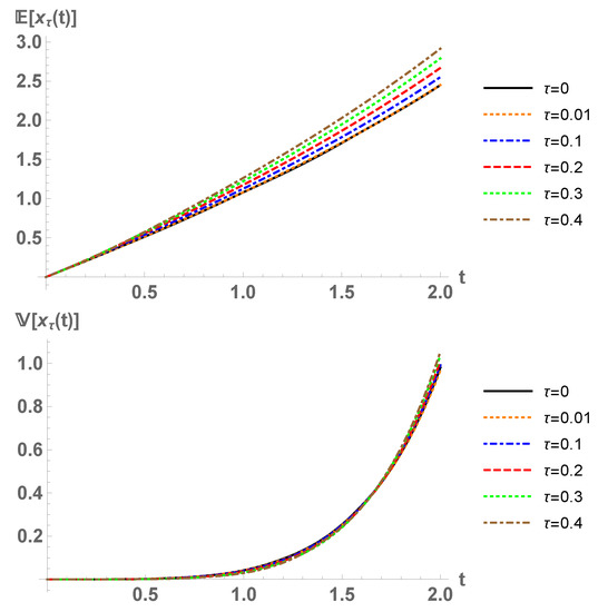
In this example, we specify new probability distributions for the input coefficients. Let $a\sim \mathrm{Uniform}(0.2,1)$, $b\sim \mathrm{Uniform}(-1,0)$, $d\sim \mathrm{Beta}(1,1.3)$ and $e\sim \mathrm{Uniform}(-0.2,-0.1)$, all of them independent. The stochastic process $x_{\tau }\left(t\right)$ given by (2) is an ${\mathrm{L}}^p$-solution for all $1\le p<\infty$, by Theorem 7. We compute $\mathbb{E}\left[x_{\tau }\left(t\right)\right]$ and $\mathbb{V}\left[x_{\tau }\left(t\right)\right]$ with (9) and (10), see Figure 2. Observe that the convergence when $\tau \to 0$ agrees with Theorem 13.

Figure 2. Expectation (up) and variance (down) of $x_{\tau }\left(t\right)$, Example 2.

We now comment on some computational aspects. We have used the software Mathematica^®, version 11.2 [37]. The integrals and expectations from (9) and (10) have been computed as multidimensional integrals with the built-in function NIntegrate (recall that the expectation is an integral with respect to the corresponding probability density function). Expression (9) does not pose serious numerical challenges, and one can use a standard NIntegrate routine with no specified options. However, for expression (10), we have set the option quasi-Monte Carlo with ${10}^5$ sampling points (otherwise the computational time would increase dramatically). We have checked numerically that the following factors increase the computational time: large ratio $t/\tau$; probability distributions with unbounded support for the input data; and moderate or large dimensions of the random space.

5. Conclusions

In this paper, we have performed a comprehensive stochastic analysis of the random linear delay differential equation with stochastic forcing term. The equation considered has one discrete delay $\tau >0$, two random coefficients a and b (corresponding to the non-delay and the delay term, respectively) and two stochastic processes $f\left(t\right)$ and $g\left(t\right)$ (corresponding to the forcing term on $[0,\infty )$ and the initial condition on $[-\tau ,0]$, respectively). Our setting supposes a step further than the previous contribution [17], in which no forcing term was considered (i.e., $f\left(t\right)=0$). We have rigorously addressed the problem of extending the deterministic theory to the random scenario, by proving that the deterministic solution constructed via the method of steps and the method of variation of constants is an ${\mathrm{L}}^p$-solution, under certain assumptions on the random data. A new result, the random Leibniz’s rule for ${\mathrm{L}}^p$-Riemann integration has been necessary to derive our conclusions. We have also studied the behavior in ${\mathrm{L}}^p$ of the random delay equation when the delay tends to zero.

Our approach has been shown to be useful to approximate the statistical moments of the solution stochastic process, in particular its expectation and its variance. Thus, it is possible to perform uncertainty quantification. Our procedure is an alternative to the usual techniques for uncertainty quantification: Monte Carlo simulation, generalized polynomial chaos (gPC) expansions, etc.

Our approach could be extendable to other random differential equations with or without delay. As usual, one could prove that the deterministic solution also works in the random framework. To do so, a rigorous and careful analysis of the probabilistic properties of the solution based on ${\mathrm{L}}^p$-calculus should be conducted.

Finally, we humbly think that advancing in theoretical aspects of random differential equations with delay will permit rigorously applying this class of equations to modeling phenomena involving memory and aftereffects together with uncertainties. In particular, they may be crucial to capture uncertainties inherent to some complex modeling problems, since input parameters of this type of equations may belong to a wider range of probability distributions than the ones considered in Itô differential equations.

References

- Smith, R.C. Uncertainty Quantification: Theory, Implementation, and Applications; SIAM: Philadelphia, PA, USA, 2013; Volume 12. [Google Scholar]
- Xiu, D. Numerical Methods for Stochastic Computations: A Spectral Method Approach; Princeton University Press: Princeton, NJ, USA, 2010. [Google Scholar]
- Le Maître, O.P.; Knio, O.M. Spectral Methods for Uncertainty Quantification: With Applications to Computational Fluid Dynamics; Springer Science & Business Media: Berlin, Germany, 2010. [Google Scholar]
- Xiu, D.; Karniadakis, G.E. Supersensitivity due to uncertain boundary conditions. Int. J. Numer. Methods Eng. 2004, 61, 2114–2138. [Google Scholar] [CrossRef]
- Soong, T.T. Random Differential Equations in Science and Engineering; Academic Press: New York, NY, USA, 1973. [Google Scholar]
- Casabán, M.C.; Cortés, J.C.; Navarro-Quiles, A.; Romero, J.V.; Roselló, M.D.; Villanueva, R.J. A comprehensive probabilistic solution of random SIS-type epidemiological models using the random variable transformation technique. Commun. Nonlinear Sci. Numer. Simul. 2016, 32, 199–210. [Google Scholar] [CrossRef]
- Strand, J.L. Random ordinary differential equations. J. Differ. Equ. 1970, 7, 538–553. [Google Scholar] [CrossRef]
- Villafuerte, L.; Braumann, C.A.; Cortés, J.C.; Jódar, L. Random differential operational calculus: Theory and applications. Comput. Math. Appl. 2010, 59, 115–125. [Google Scholar] [CrossRef]
- Saaty, T.L. Modern Nonlinear Equations; Dover Publications: New York, NY, USA, 1981. [Google Scholar]
- Cortés, J.C.; Jódar, L.; Roselló, M.D.; Villafuerte, L. Solving initial and two-point boundary value linear random differential equations: A mean square approach. Appl. Math. Comput. 2012, 219, 2204–2211. [Google Scholar] [CrossRef]
- Calatayud, J.; Cortés, J.C.; Jornet, M.; Villafuerte, L. Random non-autonomous second order linear differential equations: Mean square analytic solutions and their statistical properties. Adv. Differ. Equ. 2018, 2018, 392. [Google Scholar] [CrossRef]
- Calatayud, J.; Cortés, J.C.; Jornet, M. Improving the approximation of the first-and second-order statistics of the response stochastic process to the random Legendre differential equation. Mediterr. J. Math. 2019, 16, 68. [Google Scholar] [CrossRef]
- Licea, J.A.; Villafuerte, L.; Chen-Charpentier, B.M. Analytic and numerical solutions of a Riccati differential equation with random coefficients. J. Comput. Appl. Math. 2013, 239, 208–219. [Google Scholar] [CrossRef]
- Burgos, C.; Calatayud, J.; Cortés, J.C.; Villafuerte, L. Solving a class of random non-autonomous linear fractional differential equations by means of a generalized mean square convergent power series. Appl. Math. Lett. 2018, 78, 95–104. [Google Scholar] [CrossRef]
- Nouri, K.; Ranjbar, H. Mean square convergence of the numerical solution of random differential equations. Mediterr. J. Math. 2015, 12, 1123–1140. [Google Scholar] [CrossRef]
- Calatayud, J.; Cortés, J.C.; Jornet, M. Random differential equations with discrete delay. Stoch. Anal. Appl. 2019, 37, 699–707. [Google Scholar] [CrossRef]
- Calatayud, J.; Cortés, J.C.; Jornet, M. Lp-calculus approach to the random autonomous linear differential equation with discrete delay. Mediterr. J. Math. 2019, 16, 85. [Google Scholar] [CrossRef]
- Caraballo, T.; Cortés, J.C.; Navarro-Quiles, A. Applying the Random Variable Transformation method to solve a class of random linear differential equation with discrete delay. Appl. Math. Comput. 2019, 356, 198–218. [Google Scholar] [CrossRef]
- Zhou, T. A stochastic collocation method for delay differential equations with random input. Adv. Appl. Math. Mech. 2014, 6, 403–418. [Google Scholar] [CrossRef]
- Shi, W.; Zhang, C. Generalized polynomial chaos for nonlinear random delay differential equations. Appl. Numer. Math. 2017, 115, 16–31. [Google Scholar] [CrossRef]
- Licea-Salazar, J.A. The Polynomial Chaos Method With Applications To Random Differential Equations. Ph.D. Thesis, University of Texas at Arlington, Arlington, TX, USA, 2013. [Google Scholar]
- Khusainov, D.Y.; Ivanov, A.; Kovarzh, I.V. Solution of one heat equation with delay. Nonlinear Oscil. 2009, 12, 260–282. [Google Scholar] [CrossRef]
- Øksendal, B. Stochastic Differential Equations: An Introduction with Applications; Springer Science & Business Media: New York, NY, USA, 1998. [Google Scholar]
- Shaikhet, L. Lyapunov Functionals and Stability of Stochastic Functional Differential Equations; Springer Science & Business Media: New York, NY, USA, 2013. [Google Scholar]
- Shaikhet, L. Stability of equilibrium states of a nonlinear delay differential equation with stochastic perturbations. Int. J. Robust Nonlinear Control. 2017, 27, 915–924. [Google Scholar] [CrossRef]
- Benhadri, M.; Zeghdoudi, H. Mean square asymptotic stability in nonlinear stochastic neutral Volterra-Levin equations with Poisson jumps and variable delays. Funct. Approx. Comment. Math. 2018, 58, 157–176. [Google Scholar] [CrossRef]
- Santonja, F.J.; Shaikhet, L. Analysing social epidemics by delayed stochastic models. Discret. Dyn. Nat. Soc. 2012, 2012. [Google Scholar] [CrossRef]
- Liu, L.; Caraballo, T. Analysis of a stochastic 2D-Navier–Stokes model with infinite delay. J. Dyn. Differ. Equ. 2019, 31, 2249–2274. [Google Scholar] [CrossRef]
- Lupulescu, V.; Abbas, U. Fuzzy delay differential equations. Fuzzy Optim. Decis. Mak. 2012, 11, 99–111. [Google Scholar] [CrossRef]
- Krapivsky, P.L.; Luck, J.M.; Mallick, K. On stochastic differential equations with random delay. J. Stat. Mech. Theory Exp. 2011, 2011, P10008. [Google Scholar] [CrossRef]
- Garrido-Atienza, M.J.; Ogrowsky, A.; Schmalfuß, B. Random differential equations with random delays. Stochastics Dyn. 2011, 11, 369–388. [Google Scholar] [CrossRef]
- Calatayud, J. A Theoretical Study of a Short Rate Model. Master’s Thesis, Universitat de Barcelona, Barcelona, Spain, 2016. [Google Scholar]
- Cortés, J.C.; Villafuerte, L.; Burgos, C. A mean square chain rule and its application in solving the random Chebyshev differential equation. Mediterr. J. Math. 2017, 14, 35. [Google Scholar] [CrossRef]
- Cortés, J.C.; Jódar, L.; Villafuerte, L. Numerical solution of random differential equations: A mean square approach. Math. Comput. Model. 2007, 45, 757–765. [Google Scholar] [CrossRef]
- Braumann, C.A.; Cortés, J.C.; Jódar, L.; Villafuerte, L. On the random gamma function: Theory and computing. J. Comput. Appl. Math. 2018, 335, 142–155. [Google Scholar] [CrossRef]
- Khusainov, D.Y.; Pokojovy, M. Solving the linear 1D thermoelasticity equations with pure delay. Int. J. Math. Math. Sci. 2015, 2015. [Google Scholar] [CrossRef]
- Wolfram Mathematica, V.11.2; Wolfram Research Inc.: Champaign, IL, USA, 2017.
© 2020 by the authors. Licensee MDPI, Basel, Switzerland. This article is an open access article distributed under the terms and conditions of the Creative Commons Attribution (CC BY) license (http://creativecommons.org/licenses/by/4.0/).