Abstract
The observability of a dynamical system is affected by the presence of external inputs, either known (such as control actions) or unknown (disturbances). Inputs of unknown magnitude are especially detrimental for observability, and they also complicate its analysis. Hence, the availability of computational tools capable of analysing the observability of nonlinear systems with unknown inputs has been limited until lately. Two symbolic algorithms based on differential geometry, ORC-DF and FISPO, have been recently proposed for this task, but their critical analysis and comparison is still lacking. Here we perform an analytical comparison of both algorithms and evaluate their performance on a set of problems, while discussing their strengths and limitations. Additionally, we use these analyses to provide insights about certain aspects of the relationship between inputs and observability. We found that, while ORC-DF and FISPO follow a similar approach, they differ in key aspects that can have a substantial influence on their applicability and computational cost. The FISPO algorithm is more generally applicable, since it can analyse any nonlinear ODE model. The ORC-DF algorithm analyses models that are affine in the inputs, and if those models have known inputs it is sometimes more efficient. Thus, the optimal choice of a method depends on the characteristics of the problem under consideration. To facilitate the use of both algorithms, we implemented the ORC-DF condition in a new version of STRIKE-GOLDD, a MATLAB toolbox for structural identifiability and observability analysis. Since this software tool already had an implementation of the FISPO algorithm, the new release allows modellers and model users the convenience of choosing between different algorithms in a single tool, without changing the coding of their model.
1. Introduction
Mathematical models of ordinary differential equations (ODEs) are used in all areas of science and technology for describing nonlinear systems. The ODEs define the evolution of the system state variables with respect to time, while the measurable quantities are defined by the output function. The model equations (ODEs and output function) may contain unknown parameters and external inputs that may be known () or unknown (). The structure of the model equations determines whether it is possible to estimate the model unknowns from the outputs. The theoretical possibility of inferring the states (respectively parameters) from the outputs is called observability (respectively structural identifiability) [1,2]. Since a parameter can be considered as a state variable with time derivative equal to zero, structural identifiability can be considered as a particular case of observability. Additionally, the possibility of recovering the unknown inputs is called reconstructibility or input observability. For simplicity, in this manuscript we use the word observability for all model unknowns, that is, to refer to the possibility of determining states, parameters, and/or inputs from the output. We assume that the model structure—the ODEs and output function—is known and correct. The assessment of the possible existence of alternative structures capable of generating exactly the same output is a different albeit related problem [3] that is not addressed in the present article.
The concept of observability arose in systems and control theory. It was initially defined for linear models and extended to the nonlinear case afterwards [4]. The concept of structural identifiability, on the other hand, was motivated by the analysis of biological models [5], due to the specific challenges that parameter identification poses in mathematical biology and other biosciences. Hence, many observability analysis methods developed in that context aimed at analysing structural identifiability and were named accordingly, even though they could be applied or adapted to the more general task of analysing observability. Examples of software tools include DAISY [6], COMBOS [7], IdentifiabilityAnalysis [8], STRIKE-GOLDD [9], GenSSI [10], and SIAN [11].
The existence of external inputs affects the observability of a model and determines which methods can be applied for its analysis. A key distinction is between known and unknown inputs, where “known” is interpreted as “quantified”; thus, we are aware of the existence of an unknown input but not of its magnitude. A known input that can be manipulated is also called a control input, or simply a control. An unknown input can be considered as an unmeasured disturbance or as a time-varying parameter. Some techniques are applicable specifically to uncontrolled systems [12], while others allow for the existence of known inputs. To the best of our knowledge, the first works describing algorithms capable of handling unknown inputs were presented by [13,14]. These methods are not applicable to systems in which the outputs are direct functions of the inputs, and do not analyse the observability of the unknown input itself.
To address these issues, two differential geometry algorithms called ORC-DF—observability rank criterion with direct feedthrough [15]—and FISPO—full input, state, and parameter observability [16]—have been recently presented. Both methods are capable of determining the observability of states and parameters, and unknown inputs of nonlinear ODE models. ORC-DF is applicable to affine-in-the-inputs systems, while FISPO does not have this requirement. The latter algorithm is already implemented in the STRIKE-GOLDD toolbox [9].
In the present paper we perform a critical examination of the ORC-DF and FISPO algorithms. First we provide the necessary background on observability analysis and differential geometry in Section 2. Then we perform a theoretical analysis of the two methods in Section 3, showing that they are equivalent for systems without known inputs, and that they differ for other classes of models, as a result of building different observability matrices. Realising the convenience of having both algorithms available in the same software environment, we provide their implementations in a new version of the MATLAB toolbox STRIKE-GOLDD, which is described in Section 4. The new release includes an implementation of ORC-DF, and a seamless integration with the already existing FISPO. Furthermore, it enables the automatic analysis of multi-experiment observability throughout any of the two implemented algorithms. Since ORC-DF and FISPO are symbolic algorithms that can be computationally expensive, in Section 5 we evaluate their performances by applying them to a number of modelling problems of different domains, from mechanical engineering to biology, and report their applicability and computational costs. The analysis of the selected case studies is also helpful for obtaining detailed insights about the inner workings of the algorithms. Finally, we conclude with a discussion of the results in Section 6.
2. Materials and Methods
2.1. Notation and Model Classes
We are interested in studying the observability of nonlinear systems of the following (fairly general) form:
where f and h are nonlinear and analytical (infinitely differentiable) functions of the model variables (which depend on time ), i.e., system states a set of inputs, both known and unknown and unmeasured parameters On the other hand, the system output vector consists of measured functions of model variables. We assume that while , and are non-negative integers. Note that the dependence of model variables over time is omitted from the Equations (1)–(2) for simplicity of notation.
As a special case of we also study affine-in-inputs systems, which are given by the expressions:
where and are—possibly nonlinear—analytical functions for , and:
where, following [15]:
Note that, as in Equations (3) and (4), the functions can depend on , but we omit this dependency in the expressions above and elsewhere when convenient.
In what follows, a vector is assumed to be a one column matrix and its transpose. The Jacobian matrix of a function with respect to a vector field will be denoted as:
2.2. Background
2.2.1. Structural Identifiability, Observability, and Differential Geometry
Roughly speaking, a nonlinear system is structurally observable if it is possible to distinguish between its state trajectories from the data provided by its output, and structurally reconstructible (or input observable) if its disturbances can be tracked from the aforementioned measurements. Similarly, is said to be structurally identifiable if it is possible to infer the values of its unknown parameters from the output. In practice, it is often not necessary distinguish between every pair of unmeasured states in the phase mapping of —a property called structural global observability—and it is sufficient to distinguish neighbouring states—a property called local “weak” observability in some texts [4]. In this work we will not further make this distinction, and local “weak” structural observability will be simply called observability. Likewise, we will refer to structural local “weak” identifiability simply as identifiability.
Structural identifiability can be addressed as a particular case of observability. This is because any unknown parameter of can be considered as a zero-dynamics state, that is, the equation holds for It is then possible to augment the system state as:
which consists of components and follows the augmented dynamics:
Thus, the identifiability and observability of can be studied as the observability of the augmented system (totally equivalent to the original one) with state vector (7), dynamics (8), and output (2), the same as
The algorithms analysed in this work adopt a differential geometry approach, which relies on the use of the concept of Lie derivative to bring out algebraic (and in some sense, geometric) tests suitable to address the study of observability of analytic systems Let us consider first the simpler case in which is not dependent on unknown inputs:
Definition 1
(Lie derivative [17]). Consider the system with augmented state vector (7) and augmented dynamics (8). Fixing the control variables the Lie derivative of the output function in along the tangent vector field is:
Furthermore, setting the i-order Lie derivative of (along the vector field can be recursively computed in as:
The above definition does not capture the effect of possible time variations in the control variables. To account for it, this notion can be extended as follows:
Definition 2
(Extended Lie derivative [8]). Consider the system with augmented state vector (7), augmented dynamics (8), and assume that the controls are analytical functions on The extended Lie derivative of the output function h in by the tangent vector field is:
Moreover, setting the i-order extended Lie derivative of h can be recursively computed in as:
where stands for the -order time derivative of
Remark 1.
For any fixed controls assuming Σ is complete and denoting the state trajectory such that:
then, in the case of constant inputs the Lie derivative introduced in Definition (1) verifies:
which can be proven by using repeatedly the chain rule. Likewise, if are time-varying and the extended Lie derivative of Definition (2) verifies:
Given a nonlinear system with augmented state (7) and analytical inputs, it is possible to use the extended Lie derivatives of the output to build (symbolically) the following matrix:
which is the observability-identifiability matrix of Note that the assumption of analytic controls is conservative, since it suffices that they are differentiable up to order By calculating the rank of the above matrix, it is possible to establish the observability and identifiability of using the following condition.
Theorem 1
Remark 2.
The rank of (10) is constant except for a zero-measurement subset in the augmented state space (8) of where the rank is smaller, as a consequence of the system being analytical [18]. Thus, to verify the condition of the Theorem 1 it is sufficient to calculate the rank of (10) at any non-singular point of the phase space.
2.2.2. FISPO
Unknown inputs w can be taken into account by further augmenting the phase mapping of including w as unmeasured states. Thus, for any non-negative integer l we have the l-augmented state vector:
which follows the l-augmented dynamics:
leading to the l-augmented system:
An analogous extension for affine systems exists. Using the notation given in (5) and (6), the l-augmented system described above takes the form [13]:
where the l-augmented dynamics is decomposed as follows:
We note that, in order to build l-augmented systems and it must be possible to calculate the -time derivative of disturbances , and therefore, they will be considered as analytical functions from now on (again, this hypothesis is more restrictive than necessary). We also note that the l-augmented form of and is totally equivalent to the original system, and consists of states, controls, disturbances (the -order time derivatives of ) and m outputs, that have not changed due to state augmentation [13].
As an additional hypothesis we assume that a non-negative integer s exists (possibly such that and for all In principle, this assumption introduces a restriction on the type of allowed inputs, and it is equivalent to assuming that the disturbances are order) polynomial functions of time. Nevertheless, in practice, the method may still provide relevant information about the analytical case, as is discussed in [16].
In what follows, if a vector function depends on variables we denote:
and if (where controls u are considered to be analytical on the time interval I), then:
Definition 3
(Full input-state-parameter observability, FISPO [16]). Consider the system Σ and the augmented state vector We say that Σ has the FISPO property if, for every and can be locally determined from the output and the known inputs in a finite time interval Thus, a system Σ is FISPO if, for every and for almost any vector there is a neighbourhood such that, for all the following condition holds:
Remark 3.
The original definition of the term FISPO reproduced above refers to a model property. Here we also use it to refer to the algorithm presented for its evaluation by [16].
Using the system augmentation (12) and taking the unique such that and for all it is possible to build the following matrix,
which is the generalised observability matrix of Note that (15) coincides with the observability matrix (10) of without disturbances. Thus, the rank of provides a condition for assessing the observability of as follows:
Theorem 2
Remark 4.
For the observability of the i-th state of can also be studied using the matrix (15) Thus, if denotes the matrix obtained from after removing its i-th column, state is observable if for almost any in the phase space of
2.2.3. ORC-DF
The observability of affine systems with bounded measurable controls can also be analysed by building a different observability matrix, as explained below. For a full description of the procedure, see [15].
Definition 4
(Observability rank criterion for systems with direct feedthrough, ORC-DF). A system is classified as k-row observable if almost any initial state in the state space of the k-augmented system can be separated locally from its neighbours based on the output at consecutive times If there exists such that is k-row observable, it is said that satisfies the ORC-DF.
Lemma 1.
Consider the system , and the vector field which is recursively defined for by:
then is k-row observable if for almost any in the phase space of
Lemma 2.
If satisfies the ORC-DF, then is observable in the presence of unmeasured inputs.
Corollary 1.
Let denote the matrix that is obtained after removing the i-th column from The i-th state of is k-row observable if and only if for almost any in the phase space of
3. Theory: Analysis of the FISPO and ORC-DF Algorithms
In this section we discuss the similarities and differences between FISPO and ORC-DF, whose pseudo-code is provided in Algorithms 1 and 2.
3.1. Preliminary Remarks
We begin by recalling three facts that are relevant for the analysis: (i) The FISPO algorithm does not always require building the full matrix (15) (a full matrix can be obtained for undisturbed systems or assuming for where s is a non-negative integer), (ii) Both ORC-DF and FISPO can be inconclusive for certain models, and (iii) ORC-DF and FISPO can handle different types of inputs, although both methods allow the study of observability in the presence of generic (measurable) controls.
Remark 5
(The FISPO algorithm does not always require building the full matrix). In each iteration the FISPO algorithm builds the matrix composed by extended Lie derivatives of output up to order and then calculates its rank and partial ranks, instead of directly building the full matrix (15). The algorithm is programmed in this way because the matrix can reach full rank for some , and if the number of states increases indefinitely (15) can never be built in practice. In addition, the above procedure may classify some states as observable before obtaining the full matrix (15), since any observable state in the k-augmented system remains observable in for [13]. Moreover, if the system does not have unknown inputs it is possible to classify it as unobservable or unidentifiable using fewer than Lie derivatives [19].
Remark 6
(Both ORC-DF and FISPO can be inconclusive for certain models). If the model under study has unknown inputs and their time derivatives do not vanish for any non-negative integer both FISPO and ORC-DF algorithms can be inconclusive. This happens when the rank of the observability matrices grows at each iteration without reaching a value equal to the number of states (which also increases with each iteration). Therefore, a computational implementation of both algorithms should include shutdown conditions based on computation time or number of iterations. This impediment can also be avoided by assuming that which implies:
for any so the observability matrix constructed by FISPO at k-th iteration is:
while, in the case of affine-in-inputs systems, ORC-DF can be modified at each iteration to account for the above assumption, by taking:
Actually, ORC-DF is designed to work with unknown inputs such that are piecewise constant for but, obviously, if for a finite integer this condition is trivially verified.
| Algorithm 1 The FISPO algorithm [16]. |
 |
| Algorithm 2 The ORC-DF algorithm [15]. |
 |
Remark 7
(ORC-DF and FISPO can handle different types of inputs). Both ORC-DF and FISPO construct an observation space generated by Lie derivatives of the output; its dimension determines observability. FISPO builds an observation space spanned by extended Lie derivatives (2) considering analytical inputs, while ORC-DF assumes piecewise constant inputs and exploits certain properties specific to affine systems in order to build a different observation space. If an affine system is classified as observable by ORC-DF or FISPO, it is observable when a generic measurable input is considered [15,19].
In the next subsections we present the main novel insights of our theoretical analysis of the algorithms.
3.2. For Systems without Known Inputs, ORC-DF and FISPO Reduce to the Same Algorithm
Here we prove by induction that, if no inputs u are involved in the FISPO algorithm reduces to ORC-DF (note that is a particular case of so FISPO is directly applicable). Before presenting the result, we remark that, in the case the extended Lie derivative reduces to:
and denoting the composition of functions with ∘, the -order Lie derivative verifies:
since depends only on time derivatives for
Proof.
Setting in (5), the dynamics and output of are given by:
Let By the recursion given in Lemma (1), it is verified that:
so the induction hypothesis holds for
Consider now any non-negative integer and suppose that the induction hypothesis holds for then:
and the result is proven if for every it holds that:
3.3. For Systems with Known Inputs, ORC-DF and FISPO Lead to Different Observability Matrices
Excluding the case an important difference between the observability matrices built by algorithms ORC-DF and FISPO is the number of Lie derivatives (rows) they include in each iteration. Indeed, for
so the observability matrix constructed by FISPO grows in m rows in each iteration, while the matrix constructed by ORC-DF includes new rows in the k-th stage. This fact can be an advantage for ORC-DF, as it makes it possible to reach full rank more rapidly, i.e., with lower order Lie derivatives. However, it may also be a disadvantage if this growth makes the problem dimension increase rapidly while adding little new information. Hence the faster growth may be beneficial or not depending on the form of the mathematical expressions of the dynamics and output functions in which the known inputs are present. For example, suppose that there exists an integer and real numbers not simultaneously zero, such that:
which, using (13), implies:
Since, by definition, it holds that:
the matrix built by ORC-DF algorithm in the -th iteration includes dependent rows; the rows forming can be written as a linear combination of the remaining rows. Indeed, by a property of Lie derivative [18] it holds that:
so, using linearity of the derivative, the following linear combination has been obtained:
Likewise, if there exists such that is linearly dependent on vector fields for the observability matrix built by ORC-DF includes dependent rows in the -th iteration, for
Note that the real values can be replaced by functions of unknown parameters, as they are constant variables, so the equality (19) holds for this case as well.
4. Implementation
4.1. The STRIKE-GOLDD Software Toolbox
STRIKE-GOLDD (Structural identifiability taken as extended-generalized observability using Lie derivatives and decomposition) is an open source MATLAB toolbox that analyses the observability of nonlinear systems of the form Equations (1) and (2). It is available at https://sites.google.com/site/strikegolddtoolbox/ and https://github.com/afvillaverde/strike-goldd/. STRIKE-GOLDD versions up to v2.1.6 implemented the FISPO algorithm, including a number of additional features that go beyond the core instructions described in Algorithm 1, with the purpose of facilitating the analysis of large models. Furthermore, they also allowed one to indicate a given number of non-zero time derivatives of inputs, both known and unknown.
4.2. Implementation of the ORC-DF Algorithm
We have released a new version of STRIKE-GOLDD (v2.2) that includes an implementation of ORC-DF (Algorithm 2) along with the already existing implementation of FISPO (Algorithm 1). The algorithm is chosen with the newly introduced option opts.affine in the options.m file (set it to 1 for ORC-DF, and to 0 for FISPO). The ORC_DF.m function checks whether a model is indeed affine in the inputs, and if that is the case, converts it to the appropriate form (3) and (4) and stores it in a mat-file to avoid repeating this calculation in the future. Thus, the user only needs to enter the model once, using the same format for ORC-DF and FISPO. New specific options for the ORC-DF algorithm include the possibility of setting a maximum number of iterations through the variable opts.kmax, limiting the computation time of each stage with opts.tStage, plotting graphs of the results obtained by the algorithm with opts.graphics, and using the MATLAB Parallel Toolbox by setting the option opts.parallel to 1.
4.3. Multiple Experiments and Piecewise Constant Inputs
FISPO analyses the observability of a model for a single experiment with an infinitely differentiable ("smooth") input. However, it is possible to use it to consider multiple experiments with possibly different inputs by applying it to a modified model: if we create as many replicates of the model states, inputs, and outputs as the number of experiments that we want to consider, we obtain a new model whose analysis for a single input has the same observability properties as the original model with multiple inputs [20]. Until now, this feature was only available in the GenSSI 2.0 toolbox [10]. We have included the possibility of carrying out this multi-experiment analysis automatically (using any of the available algorithms) in the new version of STRIKE-GOLDD, by setting the option opts.multiexp=1. The number of experiments can be chosen with opts.numexp, and a set of initial conditions can be chosen by the user through the options.m file.
5. Computational Results and Discussion
We have applied the ORC-DF and FISPO algorithms to a set of illustrative case studies from different areas of science and technology, ranging from civil engineering to different biological disciplines. They are listed in Table 1, along with the computation times of the algorithms.

Table 1.
Computation times of the two algorithms for the models analysed in this study. The computation times of case studies with unknown inputs depend on the highest order of the derivatives of the unknown inputs that are assumed to be non-zero, s. Three different cases are shown for those models: . For models without unknown inputs this setting does not apply. Cases in which an algorithm cannot be applied are labelled as N/A. Results were obtained on a personal computer with 16 GB RAM and processor Intel(R) Core(TM) i7-8550U 1.80 GHz.
5.1. An Identifiable and Observable Model with Known Input: “C2M”
Our first case study is a deceivingly simple compartmental model [20]:
where each state corresponds to a compartment, and is the unknown parameter vector. The augmented state vector is with extended dynamics given by:
with the following vector fields for the affine-in-inputs formulation (5):
In addition, the output is given by the function:
The results obtained by ORC-DF and FISPO are shown in Figure 1, where the first important difference between both methods can be seen: while FISPO works with analytical, time-varying controls (which implies that it depends on functions throughout their time derivatives; see Equations (9) and (10)), ORC-DF assumes piecewise constant inputs. For this reason, the results obtained by FISPO vary according to the number of non-zero derivatives, while those of ORC-DF do not. Considering different types of inputs can be of interest in biological applications, where it is sometimes experimentally impossible to apply sufficiently exciting signals. Due to its reduced size, this model is well suited for illustrating this difference, so we derive the equations of the Lie derivatives calculated by each algorithm in Appendix A, where we also discuss other aspects and implications.
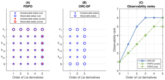
Figure 1.
Analysis of the C2M model with the FISPO and ORC-DF algorithm. For FISPO two cases are considered: , which is labelled as “(const)”, and , which is labelled as “(var)”. In the first case, higher order derivatives are assumed to be zero too. (A,B) Results of the FISPO and ORC-DF algorithms, respectively: the panel shows the states classified as observable or unobservable as a function of the number of Lie derivatives calculated by each algorithm. (C) Observability rank obtained by each algorithm as a function of the number of Lie derivatives. The full rank is equal to the number of states, i.e., six.
This model is classified as observable and identifiable by ORC-DF after three iterations. The result yielded by FISPO depends on the number of input derivatives assumed to be zero: the unmeasured variables are classified as unobservable with a constant input, while they become observable in the fifth iteration if the input is any non-constant analytical function. The variables classified as observable by both algorithms at each iteration are illustrated in Figure 1A,B. Figure 1C shows the ranks of the matrices built by both algorithms in each iteration. As can be seen, the observability matrix constructed by ORC-DF reaches full rank after considering Lie derivatives up to order three. The matrix built by FISPO stagnates from the fourth iteration onward with a constant input, while it reaches full rank after five iterations with a non-constant input.
5.2. A Non-Identifiable, Non-Observable Model with Known Inputs: “Bolie”
Our second example is a model with similarities to the previous one, given by [21]:
where is the state vector, are the unknown parameters, and u is the control variable. The augmented state vector is , and the extended dynamics are given by:
and can be separated into the vector fields:
The output is a function of the state and the unknown parameter
so, in this case, there are no directly measured states or parameters.
The model is classified as non-identifiable and non-observable by FISPO and ORC-DC, as shown in Figure 2. A detailed analysis of the calculations performed by both algorithms is provided in Appendix B.
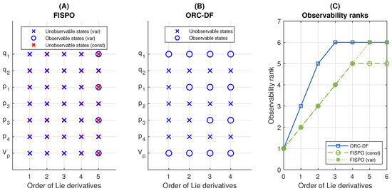
Figure 2.
Analysis of the Bolie model with the FISPO and ORC-DF algorithms. For FISPO two cases are considered: , which is labelled as “(const)”, and , which is labelled as “(var)”. In the first case, higher order derivatives are assumed to be zero too. (A,B) Results of the FISPO and ORC-DF algorithms, respectively: the panel shows the states classified as observable or unobservable as a function of the number of Lie derivatives calculated by each algorithm. (C) Observability rank obtained by each algorithm as a function of the number of Lie derivatives. The full rank is equal to the number of states, i.e., seven.
5.3. A Model with Known and Unknown Inputs: “2DOF”
We consider now an affine-in-the-inputs model with a known and an unknown input, proposed by [15]. It describes the behaviour of a mechanical system consisting of two masses connected by a spring. In the form (1) and (2), its dynamics and output functions are given by:
The state vector is and the unknown parameters are Two external forces act on the system as inputs, one of known magnitude, and another of unknown value, The remaining parameters and are known.
Since there is an unknown input acting on the model, it is necessary to include its time derivatives in the extended state vector. The 0-augmented state is , which follows the dynamics:
where the contribution of the known input is:
First we consider the case in which the unknown disturbance is assumed constant, . The results are shown in Figure 3. After calculating three Lie derivatives both algorithms conclude that the system is identifiable, observable and invertible. It should be noted that for this model FISPO always leads to the result shown in Figure 3A, regardless of the number of known input derivatives assumed to be non-zero (note that the figure shows the constant case but this property is fulfilled for any analytical disturbance
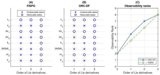
Figure 3.
Analysis of the 2DOF model. (A,B) Results of the FISPO and ORC-DF algorithms, respectively, with The panels show the states classified as observable or unobservable as a function of the number of Lie derivatives calculated by each algorithm. (C) Observability rank obtained by each algorithm as a function of the number of Lie derivatives. The full rank is equal to the number of states, i.e., eight.
Next, we consider a time-varying unknown input, assuming that for some For this case, the model is again classified as fully observable by both algorithms. However, the paths that they follow to reach that conclusion are different. The number of Lie derivatives required by FISPO to classify the model as observable increases as s grows, due to the number of states in each stage also increasing without reaching full rank, so FISPO does not reach any conclusion when In contrast, ORC-DF ends at most in four iterations, regardless of the value of (including the case This situation is illustrated in Figure 4, which shows the number of Lie derivatives required by each algorithm to achieve a result for
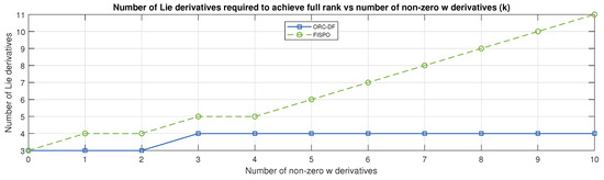
Figure 4.
Number of Lie derivatives needed by each algorithm for building the full-rank observability matrix for the 2DOF model as a function of the number of non-zero time derivatives, for
A difference between the procedures carried out by both algorithms for this model is that—similarly to the case of parameter b in the C2M example, mentioned in Appendix A—the expressions obtained by ORC-DF determine that the unknown parameter can be calculated directly from the measurements since the first iteration as:
In the case of FISPO, in contrast, the parameter is the last to be classified as identifiable, which happens at the same time in which the entry is classified as invertible for a sufficiently large s.
5.4. A Model with a Known or Unknown Input: “HIV”
Next we consider a model of HIV dynamics in the human body given by [22]:
where the states are the unknown parameters vector is and is a time-varying input, the infection rate.
As was established in Section 3.2, if is unknown, ORC-DF and FISPO become the same algorithm (leaving aside implementation details). If is known and time-varying, they differ.
This model was analysed with FISPO by [16] considering two possibilities, i.e., known and unknown. In both cases the model is classified as observable and identifiable by FISPO. In the latter case, the number of Lie derivatives necessary to achieve this conclusion grows with the number of derivatives of assumed to be non-zero, as happened with the 2DOF model analysed in Section 5.3.
It is possible to analyse the HIV model with the ORC-DF algorithm, since it is affine in input. With the infection rate considered known, i.e., , the functions of the affine formulation (13) and (14) are written as:
while if it is unknown, , we have:
If the infection rate is considered known, both algorithms classify the model as observable and identifiable, regardless of the number of input derivatives assumed non-zero by FISPO. Figure 5 illustrates this fact, where the results obtained by FISPO have been represented for a generic analytical input.
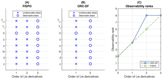
Figure 5.
Analysis of the HIV model with the FISPO and ORC-DF algorithms, with the input considered known. (A,B) Results of the FISPO and ORC-DF algorithms, respectively: the panel shows the states classified as observable or unobservable as a function of the number of Lie derivatives calculated by each algorithm. (C) Observability rank obtained by each algorithm as a function of the number of Lie derivatives. The full rank is equal to the number of states, i.e., eight.
The observability matrix calculated by ORC-DF has full rank after including Lie derivatives up to second order, so the number of its rows is (actually, 14 rows after excluding dependent rows arising from the equality while the matrix constructed by FISPO needs to include Lie derivatives up to order three to achieve full rank, so it has rows.
This is an example of a model for both algorithms perform similarly; although FISPO needs to calculate one more Lie derivative to classify the system as observable, ORC-DF calculates ranks of matrices of greater dimension, resulting in similar computational cost of the calculations involved in each algorithm. As can be seen in Figure 5C, the ranks of both observability matrices coincide up to the first iteration, as a consequence of:
5.5. A Genetic Toggle Switch with Two Inputs: “TS”
Let us now consider the following model of a genetic toggle switch [23]:
where is the state vector and the inputs are and The remaining variables are unknown parameters.
This model is an example that cannot be analysed by ORC-DF algorithm, since it is not affine in inputs. It was analysed with FISPO in [16], considering both measured and unmeasured inputs. If both inputs are known, FISPO classifies the model as structurally identifiable, as long as neither input is constant. If the inputs are unknown FISPO concludes that some parameters become unidentifiable. For more details we refer the reader to [16].
5.6. A Signalling Pathway with Five Known Inputs: “JAK-STAT”
To show the computational limitations of the two algorithms, we analyse here a model that pushes them to their limits. It is a classic model of the JAK-STAT signalling pathway presented by [24], which has 25 states, 26 unknown parameters, and 5 inputs. The output consists on 15 measured functions of the model variables that depend only on one of the external signals which is not involved in system dynamics, that is,
The model equations are provided in Appendix C.
This model was analysed with FISPO in [25], concluding that all its parameters are structurally identifiable but two of its 25 states are non-observable. The calculations are computationally expensive, requiring the use of procedures supported in STRIKE-GOLDD—such as model decomposition or successive executions after removing parameters previously classified as identifiable—in order to reach the conclusion. Thus, the model was first analysed after setting the maximum computation time of each Lie derivative to 100 seconds, which allowed FISPO to calculate 5 Lie derivatives and to classify 17 parameters and 4 states as observable. Next, the 17 parameters were specified as previously classified in the FISPO options, thereby removing them from further consideration and decreasing the size of the problem, and the model was decomposed. The post-decomposition analysis classified five additional parameters as identifiable. After removing them, it was possible to analyse the remainder of the model and reach the aforementioned conclusion.
With ORC-DF we did not manage to analyse the model due to computational limitations (specifically, insufficient memory). The different computational requirements of ORC-DF and FISPO are shown in Table 2.
Table 2.
Results and computation times of ORC-DF and FISPO for the JAK-STAT model.
Table 2 shows that the number of rows of the matrix built by ORC-DF grows rapidly at each iteration (even though the implementation removes null rows arising from dependencies in (20) and (21), which is why the number of rows of the ORC-DF matrix does not match the number given in Section 3.3). Although this matrix leads to higher ranks than the one built by FISPO, especially at the beginning of the execution (i.e., with few Lie derivatives), the difference decreases soon and the ranks of the two matrices are similar despite the big difference in the number of rows. With five Lie derivatives, ORC-DF labels 27 model variables as observable (9 states and 18 parameters), including those classified as observable by FISPO (21: 4 states and 17 parameters). However, the computation time of ORC-DF at that point is roughly ten times higher than FISPO, and memory requirements impede further progress with this algorithm.
6. Conclusions
In this paper we have analysed two recent algorithms for observability analysis of nonlinear systems with known and/or unknown inputs, which we refer to as ORC-DF and FISPO. Our analyses have revealed the key similarities and differences between them. The main conclusions can be summarized as follows.
First, we have proven theoretically that for models without known inputs both algorithms are basically equivalent, since they calculate the rank of the same observability matrix. In contrast, for models with known inputs—e.g., for controlled systems—the two algorithms differ, since they build different observability matrices. Specifically, the number of rows of the matrix built by ORC-DF increases more at each iteration than the one built by FISPO. We have shown that this increased growth is often an advantage of ORC-DF, since it makes it possible to reach full rank—and thus, to conclude that a model is observable—with less Lie derivatives, and hence less computational cost; an example was shown in Section 5.1. However, said increased growth is not always advantageous: as we have noted in Section 3.3, it can also be detrimental to the efficiency of ORC-DF. The latter situation may happen when the structure of the model equations is such that the increase in problem dimension outweighs the increase in information resulting from the inclusion of a new Lie derivative; we provided an example in Section 5.6.
When applying FISPO to a model with unknown input(s) it is usually necessary to assume that their derivatives, , are zero for orders higher than a finite s, which amounts to assuming that the unknown inputs are polynomial functions. This is not a theoretical requirement—and in fact, a counter-example that did not require this assumption was shown in [16]—but it is often necessary in practice in order to reach a conclusion in finite time. This was indeed the case for the models with unknown inputs that we analysed in this paper. It should be noted that the results obtained under this assumption are not necessarily valid if the unknown input has nonzero derivatives of order higher than s.
We remark that this assumption of polynomial inputs does not apply to known inputs; FISPO does not require this assumption for their analysis, and it is not used by ORC-DF either. That being said, it must be taken into account that in certain applications there are experimental limitations that do not allow one to use sophisticated input signals for system identification. This situation is common in biological modelling, where often times only constant or ramp inputs can be applied. The implications of such limitations in observability can be taken into account by specifying that the derivatives of the known inputs, , are zero for orders higher than a finite s. This option is available in STRIKE-GOLDD.
Another difference between both algorithms lies in the types of models and known inputs that they can analyse. In regard to model types, FISPO is applicable to a general class of nonlinear ODE models, while ORC-DF is applicable to a subclass of those models: the ones that are affine in the inputs. There is an additional, albeit subtle, difference between both algorithms in regard to the known inputs: FISPO considers infinitely differentiable ("smooth") functions, while ORC-DF considers piecewise constant inputs. It should be noted however that an affine system that is observable for piecewise constant inputs is also observable for smooth inputs; therefore, ORC-DF can also establish the observability of (affine) models with continuous inputs.
In a new release of the STRIKE-GOLDD toolbox (v2.2) we have included an implementation of the ORC-DF algorithm, thus allowing the user to apply different algorithms with the same tool and model definition. It should be noted that the implementations of the FISPO and ORC-DF algorithms included in the STRIKE-GOLDD toolbox have a number of additional features that increase the efficiency of the core algorithms analysed here, as noted in Section 4. We used the new implementations in STRIKE-GOLDD 2.2 to benchmark the algorithms with several models taken from the literature. Our selection of case studies included both simple models, used for illustrating the inner workings of the algorithms in detail, and more complex models whose analysis is computationally challenging, which we used for pushing the algorithms to their limits. We also provided an example of a model that cannot be analysed with ORC-DF due to being not affine in the inputs.
In conclusion, the theoretical and computational analyses presented here have informed us about the differences between the ORC-DF and FISPO algorithms, showing that they represent complementary techniques for solving an often challenging problem, and clarifying when one may be preferred over the other. The release of a new version of the MATLAB toolbox STRIKE-GOLDD that includes implementations of both algorithms provides the convenience of performing different analyses with minimal intervention from the user.
Author Contributions
A.F.V. designed and supervised the research; N.M. implemented the software and performed the computational experiments; N.M. and A.F.V. analysed the algorithms and the results; N.M. and A.F.V. wrote the manuscript. All authors have read and agreed to the published version of the manuscript.
Funding
This research was supported by the Spanish Ministry of Science, Innovation and Universities through the project SYNBIOCONTROL (reference DPI2017-82896-C2-2-R). We acknowledge support of the publication fee by the CSIC Open Access Publication Support Initiative through its Unit of Information Resources for Research (URICI) and by the Xunta de Galicia through grant ref. IN607B 2020-03.
Conflicts of Interest
The authors declare no competing interests.
Data and Materials Availability
The methods and models used in this paper are available in the GitHub repository as part of release v2.2 of the STRIKE-GOLDD toolbox: https://github.com/afvillaverde/strike-goldd.
Appendix A. Analysis of the Lie Derivatives of the C2M Case Study
Let us first consider the FISPO algorithm and the model with a non-constant input. As shown in Figure 1C, in this case there are six independent extended Lie derivatives of the output, which are given by:
Therefore, from the above system we can extract directly the following input–output expressions:
where are functions that depend only on the output, the input, and their time derivatives. It is possible to obtain similar input–output expressions for any variable involved in the model by determining the unique solution of the system (A7)–(A12), which consists of six independent equations and six unknowns. Note that the assumption for does not imply loss of generality, because the presence of higher order derivatives does not affect the unicity of the solution of (A1)–(A6) (if anything, they would contribute to the independence of the equations).
By inspecting Equations (A7)–(A12) it is possible to explain the classification obtained by FISPO and shown in Figure 1A (blue line), since it is not possible to obtain such an input–output expression for any unmeasured variable until calculating the fifth Lie derivative (A6), when the ambiguities in the equations are finally resolved. (Note that this result requires excluding those states and parameters in the phase space for which the denominators in the input–output expressions vanish. However, since the system is analytical these states form a zero measurement subset.)
Let us consider now the FISPO algorithm in the constant input case. From Figure 1C it follows that the equations obtained (A1)–(A6) are dependent. The following system of equations is extracted from (A1)–(A5):
Using Equations (A17) and (A19–A21), it is possible to write the combinations y exclusively in terms of the input and output of the model. Thus, after replacing in (A18), the system to be solved is:
which has six unknowns and five independent equations (infinite solutions), so it is not possible to write (at least, locally) any of the parameters or the unknown state as a function of the input and output. This scenario is shown in Figure 1A (red line).
We consider now the ORC-DF algorithm. Instead of (A1)–(A6), this method computes the following Lie derivatives (independent of the control values, since they are assumed to be piecewise constant):
The system (A27)–(A33) has a unique solution, in which one of the equations depends on the others. The solution, obtained from (A27)–(A31) and (A33), is given as a function of Lie derivatives as follows:
Therefore, the ORC-DF algorithm classifies the C2M model as observable and identifiable after the third iteration. We note that Equation (A29) implies that parameter b can be calculated directly from the output.
Appendix B. Analysis of the Lie Derivatives of the Bolie Case Study
Assuming non-constant input, FISPO calculates six independent Lie derivatives of the output, as shown in Figure 2C:
System (A34)–(A39) has infinite solutions, since it is composed by six equations and seven unknowns, but similarly to the C2M case study, it is possible to perform a series of algebraic manipulations on the above equations to obtain an input–output expression for the variables and as it shown in Figure 2.
In the case of constant input, Equations (A34)–(A39) become redundant, so there are only five independent Lie derivatives, as is shown in Figure 2. The combinations are the only observable functions of the variables that can be extracted from (A34)–(A38). Since the rational combinations of these functions are insufficient to determine any of the parameters or states, all variables are non-observable, as shown in Figure 2A (red line).
On the other hand, ORC-DF calculates the following Lie derivatives:
From Equations (A40), (A42), and (A44) it is easy to obtain the state and the parameters and uniquely from the measurements, using Lie derivatives up to order two. This property is not fulfilled by the system formed by (A34)–(A39); Figure 2A shows that the aforementioned variables are classified as observable by FISPO only after considering fifth order derivatives. Using the input–output expressions of , and extracted from (A40), (A42) and (A44), in conjunction with Equations (A41), (A43) and (A46), it is also possible to determine parameter as a function of the Lie derivatives of the output. However, Figure 2C shows that system (A40)–(A46) contains one redundant equation, so it is not possible to determine uniquely an input–output expression of the remaining unmeasured states. It can also be noted that any rational combination of the observable variables with the functions and is also observable.
Appendix C. Equations of the JAK-STAT Model
The dynamics of the JAK-STAT model analysed in Section 5.6 is given by:
where the auxiliary variables and have been used.
The 25 states are, respectively, the following species: EpoRJAK2, EpoRpJAK2, p1EpoRpJAK2, p2EpoRpJAK2, p12EpoRpJAK2, EpoRJAK2_CIS, SHP1, SHP1Act, STAT5, pSTAT5, npSTAT5, CISnRNA1, CISnRNA2, CISnRNA3, CISnRNA4, CISnRNA5, CISRNA, CIS, SOCS3nRNA1, SOCS3nRNA2, SOCS3nRNA3, SOCS3nRNA4, SOCS3nRNA5, SOCS3RNA, and SOCS3.
The 27 unknown parameters, , were written in the original publication [24] as: CISEqc, CISEqcOE, CISInh, CISRNADelay, CISRNATurn, CISTurn, EpoRActJAK2, EpoRCISInh, EpoRCISRemove, JAK2ActEpo, JAK2EpoRDeaSHP1, SHP1ActEpoR, SHP1Dea, SHP1ProOE, SOCS3Eqc, SOCS3EqcOE, SOCS3Inh, SOCS3RNADelay, SOCS3RNATurn, SOCS3Turn, STAT5ActEpoR, STAT5ActJAK2, STAT5Exp, STAT5Imp, init_EpoRJAK2, init_SHP1, and init_STAT5.
The model has seven known constants (–), five of which correspond to experimental conditions that can be considered as constant inputs (–), including the external signal ( Epo).
The output equations are:
References
- Chatzis, M.N.; Chatzi, E.N.; Smyth, A.W. On the observability and identifiability of nonlinear structural and mechanical systems. Struct. Control Health Monit. 2015, 22, 574–593. [Google Scholar] [CrossRef]
- Villaverde, A.F. Observability and Structural Identifiability of Nonlinear Biological Systems. Complexity 2019, 2019, 8497093. [Google Scholar] [CrossRef]
- Tuza, Z.A.; Ács, B.; Szederkényi, G.; Allgöwer, F. Efficient computation of all distinct realization structures of kinetic systems. IFAC-PapersOnLine 2016, 49, 194–200. [Google Scholar] [CrossRef]
- Hermann, R.; Krener, A.J. Nonlinear controllability and observability. IEEE Trans. Autom. Control 1977, 22, 728–740. [Google Scholar] [CrossRef]
- Bellman, R.; Åström, K.J. On structural identifiability. Math. Biosci. 1970, 7, 329–339. [Google Scholar] [CrossRef]
- Bellu, G.; Saccomani, M.P.; Audoly, S.; D’Angio, L. DAISY: A new software tool to test global identifiability of biological and physiological systems. Comput. Methods Programs Biomed. 2007, 88, 52–61. [Google Scholar] [CrossRef] [PubMed]
- Meshkat, N.; Eisenberg, M.; DiStefano, J.J. An algorithm for finding globally identifiable parameter combinations of nonlinear ODE models using Gröbner Bases. Math. Biosci. 2009, 222, 61–72. [Google Scholar] [CrossRef] [PubMed]
- Karlsson, J.; Anguelova, M.; Jirstrand, M. An Efficient Method for Structural Identiability Analysis of Large Dynamic Systems. In Proceedings of the 16th IFAC Symposium on System Identification, Brussels, Belgium, 11–13 July 2012; Volume 16, pp. 941–946. [Google Scholar]
- Villaverde, A.F.; Barreiro, A.; Papachristodoulou, A. Structural identifiability of dynamic systems biology models. PLoS Comput. Biol. 2016, 12, e1005153. [Google Scholar] [CrossRef] [PubMed]
- Ligon, T.S.; Fröhlich, F.; Chiş, O.T.; Banga, J.R.; Balsa-Canto, E.; Hasenauer, J. GenSSI 2.0: Multi- experiment structural identifiability analysis of SBML models. Bioinformatics 2018, 8, 1421–1423. [Google Scholar] [CrossRef] [PubMed]
- Hong, H.; Ovchinnikov, A.; Pogudin, G.; Yap, C. SIAN: A tool for assessing structural identifiability of parametric ODEs. ACM Commun. Comput. Algebra 2019, 53, 37–40. [Google Scholar] [CrossRef]
- Evans, N.D.; Chapman, M.J.; Chappell, M.J.; Godfrey, K.R. Identifiability of uncontrolled nonlinear rational systems. Automatica 2002, 38, 1799–1805. [Google Scholar] [CrossRef]
- Martinelli, A. Extension of the observability rank condition to nonlinear systems driven by unknown inputs. In Proceedings of the 2015 23rd Mediterranean Conference on Control and Automation (MED), Torremolinos, Spain, 16–19 June 2015; pp. 589–595. [Google Scholar]
- Martinelli, A. Nonlinear Unknown Input Observability: Extension of the Observability Rank Condition. IEEE Trans. Autom. Control 2019, 64, 222–237. [Google Scholar] [CrossRef]
- Maes, K.; Chatzis, M.; Lombaert, G. Observability of nonlinear systems with unmeasured inputs. Mech. Syst. Signal Process. 2019, 130, 378–394. [Google Scholar] [CrossRef]
- Villaverde, A.F.; Tsiantis, N.; Banga, J.R. Full observability and estimation of unknown inputs, states, and parameters of nonlinear biological models. J. R. Soc. Interface 2019, 16, 20190043. [Google Scholar] [CrossRef] [PubMed]
- Vidyasagar, M. Nonlinear Systems Analysis; Prentice Hall: Englewood Cliffs, NJ, USA, 1993. [Google Scholar]
- Isidori, A. Nonlinear Control Systems; Springer Science & Business Media: Berlin/Heidelberg, Germany, 1995. [Google Scholar]
- Anguelova, M. Nonlinear observability and identifiability: General theory and a case study of a kinetic model for S. cerevisiae. Master’s Thesis, Chalmers University of Technology and Göteborg University, Göteborg, Sweden, 2004. [Google Scholar]
- Villaverde, A.F.; Evans, N.D.; Chappell, M.J.; Banga, J.R. Input-Dependent Structural Identifiability of Nonlinear Systems. IEEE Control Syst. Lett. 2019, 3, 272–277. [Google Scholar] [CrossRef]
- Bolie, J. Coefficients of normal blood glucose regulation. J. Appl. Physiol. 1961, 16, 783–788. [Google Scholar] [CrossRef] [PubMed]
- Miao, H.; Xia, X.; Perelson, A.S.; Wu, H. On identifiability of nonlinear ODE models and applications in viral dynamics. SIAM Rev. 2011, 53, 3–39. [Google Scholar] [CrossRef] [PubMed]
- Lugagne, J.B.; Carrillo, S.S.; Kirch, M.; Köhler, A.; Batt, G.; Hersen, P. Balancing a genetic toggle switch by real-time feedback control and periodic forcing. Nat. Commun. 2017, 8, 1671. [Google Scholar] [CrossRef] [PubMed]
- Bachmann, J.; Raue, A.; Schilling, M.; Böhm, M.E.; Kreutz, C.; Kaschek, D.; Busch, H.; Gretz, N.; Lehmann, W.D.; Timmer, J.; et al. Division of labor by dual feedback regulators controls JAK2/STAT5 signaling over broad ligand range. Mol. Syst. Biol. 2011, 7, 516. [Google Scholar] [CrossRef] [PubMed]
- Villaverde, A.F.; Banga, J.R. Análisis de observabilidad e identificabilidad estructural de modelos no lineales: Aplicación a la vía de señalización JAK/STAT. In XL Jornadas de Automática. Universidade da Coruña; Servizo de Publicacións—UDC: Coruña, Spain, 2019; pp. 631–638. [Google Scholar]
Publisher’s Note: MDPI stays neutral with regard to jurisdictional claims in published maps and institutional affiliations. |
© 2020 by the authors. Licensee MDPI, Basel, Switzerland. This article is an open access article distributed under the terms and conditions of the Creative Commons Attribution (CC BY) license (http://creativecommons.org/licenses/by/4.0/).