Revealing Spectrum Features of Stochastic Neuron Spike Trains

Abstract

Power spectra of spike trains reveal important properties of neuronal behavior. They exhibit several peaks, whose shape and position depend on applied stimuli and intrinsic biophysical properties, such as input current density and channel noise. The position of the spectral peaks in the frequency domain is not straightforwardly predictable from statistical averages of the interspike intervals, especially when stochastic behavior prevails. In this work, we provide a model for the neuronal power spectrum, obtained from Discrete Fourier Transform and expressed as a series of expected value of sinusoidal terms. The first term of the series allows us to estimate the frequencies of the spectral peaks to a maximum error of a few Hz, and to interpret why they are not harmonics of the first peak frequency. Thus, the simple expression of the proposed power spectral density (PSD) model makes it a powerful interpretative tool of PSD shape, and also useful for neurophysiological studies aimed at extracting information on neuronal behavior from spike train spectra.

1. Introduction

A sequence of action potentials is the main way neurons communicate each other. Neuroscientists agree that information is conveyed by the positions in the time of the action potentials, rather than by their waveform, so that often a sequence of unitary impulses located at the instant of the spikes onset, here referred to as neuronal spike train, is used as idealized neuron output [1].

Oscillations in neuronal spike train firing rate reflect encoding properties of single neurons and/or neuronal networks [2,3,4,5,6,7,8,9] and reveal different physiological and pathological conditions [10,11,12]. Indeed, this code reflects not only the neuron’s input stimuli, but also the neuron’s biophysical properties [1], so that one of the open questions in neuroscience is the evaluation of the extent to which a neuron’s spiking response is due to the applied stimulus and to its intrinsic biophysical properties [13].

Estimation of the spike train power spectrum is a powerful method for analyzing neuronal outputs, used on a variety of neurophysiological recordings, such as multiunit activity (MUA), single unit spike trains and cellular membrane potentials [14,15,16,17,18,19,20], as well as on the output of different neuronal models to characterize the response of the modeled neuron to input stimuli [5,21,22,23,24,25] Recently, spectral analysis was applied also to experimental recordings from Globus pallidum neurons of Parkinson’s patients [18] and the general form of the power spectrum shape was suggested as a classification criterion of neural systems and their activity [18,19,20]. Power spectral analysis is also at the basis of several techniques aimed at the understanding of neuronal encoding properties of weak input signals [4,5,23,26,27]. Among them we may mention the classical signal to noise ratio (SNR), calculated as the ratio of the output power spectrum at the input frequency and the background noise spectrum [4,21,28,29], the coherence function between the input signal $s(t)$ and the output $y(t)$, calculated from second-order spectral measures of input and output [30], and advanced techniques based on homomorphic deconvolution [23,31].

Spectral estimates based on the Discrete Time Fourier Transform (DFT) and its fast implementation, the Fast Fourier Transform (FFT) are versatile and efficient techniques, largely used for evaluating the power spectral density (PSD) of neuronal spike trains coming from model simulations or experimental recordings. The typical shape of a neuronal spectrum presents a main peak which was interpreted as the mode of firing rate and less well-defined peaks approximately centered around the harmonics of the first one [32]. Our previous studies on spike trains coming from stochastic Hodgkin and Huxley (HH) neuron models [22,23,31,32] have shown that positions of such peaks depend, in a not trivial way, on the level of stimulation current and on the noise level, related to the size of membrane patch. Moreover, neuronal spectral features cannot be directly obtainable from statistical averages of the interspike interval (ISI).

To reveal such spectral features, we derive a model that expresses the PSD of a neuronal spike train as a series of expected values of cosines, function of frequency and multiples of the ISI random variable. The model, valid under the well-assessed assumptions that the ISI random variables are independent and identically distributed (i.i.d.), allows us to obtain a PSD model, which perfectly matches the FFT estimate obtained over one thousand neuronal traces. Moreover, the first term only of the series allows an accurate and straightforward estimation of the spectral peaks positions, giving a useful interpretation of the relationship between neuronal spectral components and ISI distribution.

In this paper, PSDs have been calculated and tested on the outputs of a stochastic HH model, under several conditions of background stimulation (stimulation current density) and channel noise (size of the membrane patch), but it is applicable to any kind of spike trains coming from different neuronal models, such as integrate-and-fire [33,34], multi-compartment models [35], or experimental recordings. The paper is organized as follows. In Section 2 the PSD model is derived. Results are shown and commented in Section 3. In particular, in Section 3.1, neuronal spectral features coming from the classical FFT based estimation of PSD are recalled and their dependence on the HH model parameters is analyzed. Section 3.2 presents the PSD model estimation of neuronal spectral features. Finally, in Section 4, conclusions are drawn.

2. Model and Methods

2.1. Spike Train PSD Model

Substituting each action potential instance with a unitary impulse, located at the instant of the spikes onset, is a common practice to extract neuronal encoding from the neuron output. These instants are not deterministic but they can be considered as random variable (r.v.), therefore the spike train is a stochastic process, very often considered as a stochastic point process [1]. In particular, since data come from simulations or sampled neuronal recordings, we can consider the point process as a discrete time process, provided that at most one event occurs in each sampling period $T_s$; this condition is also called orderly. The point process represents the ordered times of occurrence of spikes as integer multiple of the sampling interval [36]. We can define the difference between two spike occurrences, called interspike interval (ISI), as

$${\mathsf{\Theta }}_i={\theta }_{i+1}-{\theta }_i.$$

(1)

where ${\theta }_i$ is the time of a spike occurrence. Let us assume the r.v. ${\mathsf{\Theta }}_i$ as independent and identically distributed (i.i.d.).

A point process (p.p.) may be defined formally as a random non-negative integer-valued measure [37]. For a p.p., the counting variate, $u(0,t]$ counts the number of events in the interval $(0,t]$. An important elementary function of a p.p. is the differential increment. The differential increment, denoted by $\mathrm{d}u(t)$, is defined as $\mathrm{d}u(t)=u(t,t+\mathrm{d}t]$, where in discrete time processing $\mathrm{d}t$ can be assumed equal to the sampling period, $T_s$ [36]. In the following we will use the current notation for discrete time signals, i.e., the normalised time, $n=\lfloor (t/T_s)$ and frequency, ${\omega }_k=2\pi \frac{k}{N}$, where N is the observation interval and ⌊ is the floor operator that implements the integer division between t and $T_s$.

For an orderly p.p., $\mathrm{d}u[n]$ will take the value 0 or 1 depending on the occurrence of a spike in the sampling interval [36]; thus, for a given observation interval, the differential increment of the p.p. can be also written as

$$\mathrm{d}u[n]=\sum _{i=1}^M\delta [n-{\theta }_i]$$

(2)

where the r.v. ${\theta }_i$ represents the normalized time occurrence of i-th spike, M is the number of spikes occurring in N, and $\delta$ is the discrete time unitary impulse.

The DFT is an important means for the study of point processes. The DFT of a weakly stationary p.p. can be defined as [37]

$$U[k]=\sum _{n=0}^{N-1}{\mathrm{e}}^{-j{\omega }_{k}n}\mathrm{d}u[n]$$

(3)

where ${\omega }_k=\frac{2\pi }{N}k$ with $k=0\dots N/2$ are the discrete frequencies. The normalized discrete frequencies ${\omega }_k$ can be expressed in hertz by doing $f_k=\frac{{\omega }_k}{2\pi T_{\mathrm{s}}}$, like the normalized spike occurrence or ISI in second by multiplying them by $T_{\mathrm{s}}$. By substituting (2) in (3), we obtain (see also (25) in [36])

$$U[k]=\sum _{i=1}^M{\mathrm{e}}^{-j{\omega }_k{\theta }_i}.$$

(4)

Finally, the power spectrum of the p.p. can be defined as

$$S_u[k]={E\{|U[k]|}^2\}$$

(5)

This spectrum has a characteristic shape with one dominant peak around the mode of rate of firing and other less well-defined peaks centered around the harmonics of the first one [22,23,31,32,36].

If one wants to describe ${\left|U[k]\right|}^2$ as a function of ISI, the (4) can be further developed:

$$\begin{array}{cc}{\left|U[k]\right|}^2\hfill & =\left({\sum }_{i=1}^M{\mathrm{e}}^{-j{\omega }_k{\theta }_i}\right)\left({\sum }_{i=1}^M{\mathrm{e}}^{j{\omega }_k{\theta }_i}\right)=M+2{\sum }_{i=1}^{M-1}{\sum }_{j=i+1}^{M}cos{\omega }_k({\theta }_i-{\theta }_j)\hfill \\ \hfill & =M+2\sum _{i=1}^{M-1}\sum _{j=i+1}^{M}cos{\omega }_k\left(\sum _{q=i}^{j-1}{\mathsf{\Theta }}_q\right)\hfill \end{array}$$

(6)

From this formula one can notice that the final spectrum is the combination of cosine functions, dependent on the ISI distribution and the number of spikes of the realizations.

To clarify which terms make it up, the (6) can be written as

$$\begin{array}{c}{\left|U[k]\right|}^2=M+2\left({\sum }_{i=1}^{M-1}cos{\omega }_k{\mathsf{\Theta }}_i+{\sum }_{i=1}^{M-2}cos{\omega }_k\left({\mathsf{\Theta }}_i+{\mathsf{\Theta }}_{i+1}\right)+{\sum }_{i=1}^{M-3}cos{\omega }_k\left({\mathsf{\Theta }}_i+{\mathsf{\Theta }}_{i+1}+{\mathsf{\Theta }}_{i+2}\right)+\dots \right)\hfill \end{array}$$

(7)

The spectral representation in (7) is a stochastic process consisting of the sum of many components. Let us consider a generic term of (7).

$${\mathsf{{\rm Y}}}_p({\omega }_k)=\sum _{i=1}^{M-p}cosp{\omega }_k{\mathsf{\Theta }}_i.$$

(8)

Given a finite and different from zero value of ${\omega }_k$, the terms of the series are i.i.d. r.v., being a deterministic function of the i.i.d. random variables ${\mathsf{\Theta }}_i$. In addition, the integer M is a r.v., but not independent from ${\mathsf{\Theta }}_i$. Therefore M can also be written as a stopping time for the sum of ${\mathsf{\Theta }}_i$:

$$M=min\left\{n:\sum _{i=1}^n{\mathsf{\Theta }}_i>N\right\}-1.$$

(9)

Under this assumption the validity of Wald’s equation [38] holds, and we can write the expected value of ${\mathsf{{\rm Y}}}_p({\omega }_k)$ as

$$E\left\{{\mathsf{{\rm Y}}}_p({\omega }_k)\right\}=\left(E\left\{M\right\}-p\right)E\left\{cosp{\omega }_k\mathsf{\Theta }\right\}=\left(\overline{M}-p\right)E\left\{{\chi }_p({\omega }_k)\right\}$$

(10)

where ${\chi }_p({\omega }_k)=cosp{\omega }_k\mathsf{\Theta }$ and $\overline{M}$ is the expected value of M. Calling ${\mathsf{\mu }}_p({\omega }_k)=E[{\chi }_p({\omega }_k)]$ and ${\sigma }_p^2({\omega }_k)=\mathrm{var}[{\chi }_p({\omega }_k)]$, respectively the expected value and the variance of ${\chi }_p({\omega }_k)$, ${\mathsf{{\rm Y}}}_p({\omega }_k)$ properly shifted and normalized is

$${\upsilon }_p({\omega }_k)=\frac{{\mathsf{{\rm Y}}}_p({\omega }_k)-(\overline{M}-p){\mathsf{\mu }}_p({\omega }_k)}{{\sigma }_p({\omega }_k)\sqrt{\overline{M}-p}}$$

(11)

which, considering a sequence with an infinite number of spikes, M, for the central limit theorem, tends toward a standard normal distribution $\mathcal{N}(0,1)$.

Eventually, since the sum of normal r.v. is a normal r.v. with expected value equal to the sum of the expected values, we can approximate the PSD of the spike train, taking only the first P terms of (7),

$$S_u^P[k]={E\{|U[k]|}^2\}=E\{M+2\sum _{p=1}^{M-1}{\mathsf{{\rm Y}}}_p({\omega }_k)\}\simeq \overline{M}+\sum _{p=1}^{P}2(\overline{M}-p){\mathsf{\mu }}_p({\omega }_k).$$

(12)

obtaining the desired PSD model.

2.2. Test Data

The spike trains ($\mathrm{d}u[t]$) used as test were obtained from the complete stochastic HH model described in detail in [23,31]. Stochasticity of sodium and potassium currents was accounted for by solving a channel-state-tracking algorithm [39,40] with the Monte Carlo approach [41]. The bias current density $I_0$, describing the excitability level of the neuron, was set to constant values (7, 10, 20) μA/cm². All these values are considered supra-threshold, i.e., they induce a sustained firing mode even in the absence of internal noise [42]. The higher $I_0$ the more frequent the induced firing activity will be. Three values for the membrane patch size were considered: (11, 100, 300) μm². Assuming constant spatial densities for the sodium (60 N_Na/μm²) and potassium (18 N_k/μm²) channels, patch area determines the channel noise level, which is inversely proportional to its square root [43,44]. The model was run in the C ++ environment using the explicit Euler integration method with time step $T_s$ equal to 10 μs. In our simulation conditions this numerical method is sufficiently accurate, although higher order methods may be necessary when considering time dependent $I_0$ [45]. The observation interval $N{T}_s$ is equal to 2 s, resulting in a spectrum frequency resolution of 0.5 Hz.

3. Results

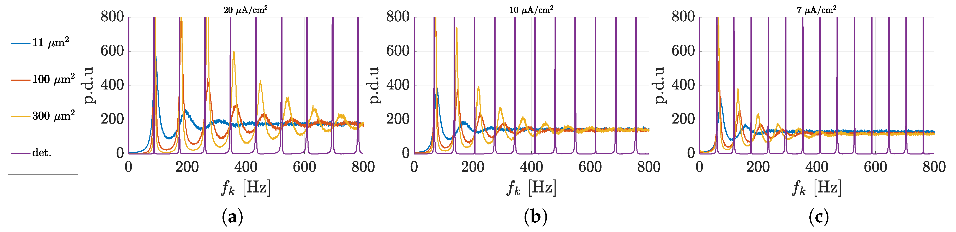
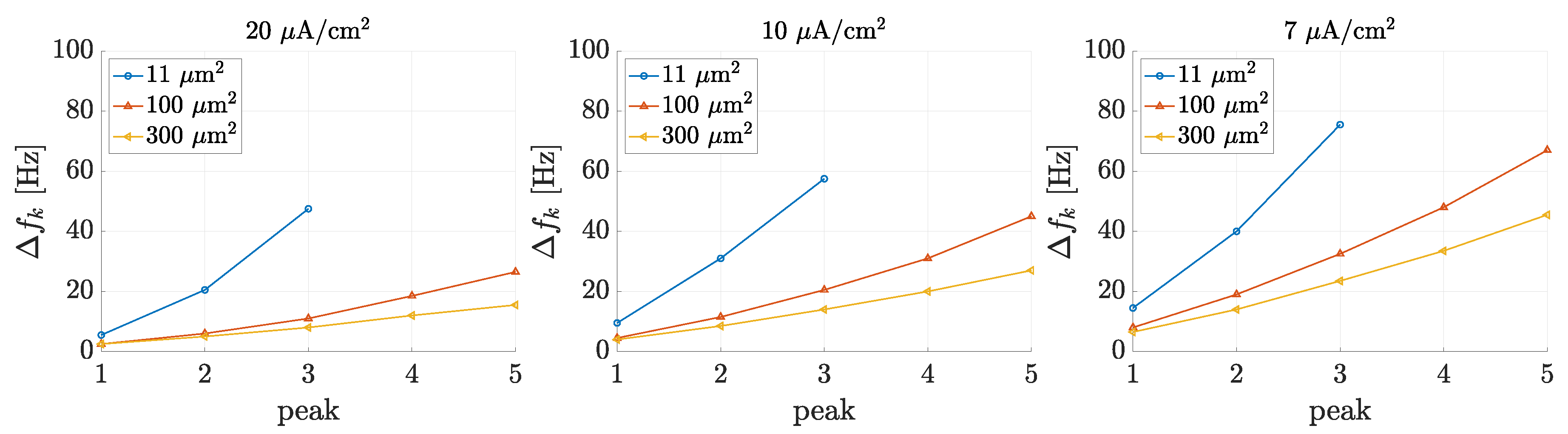
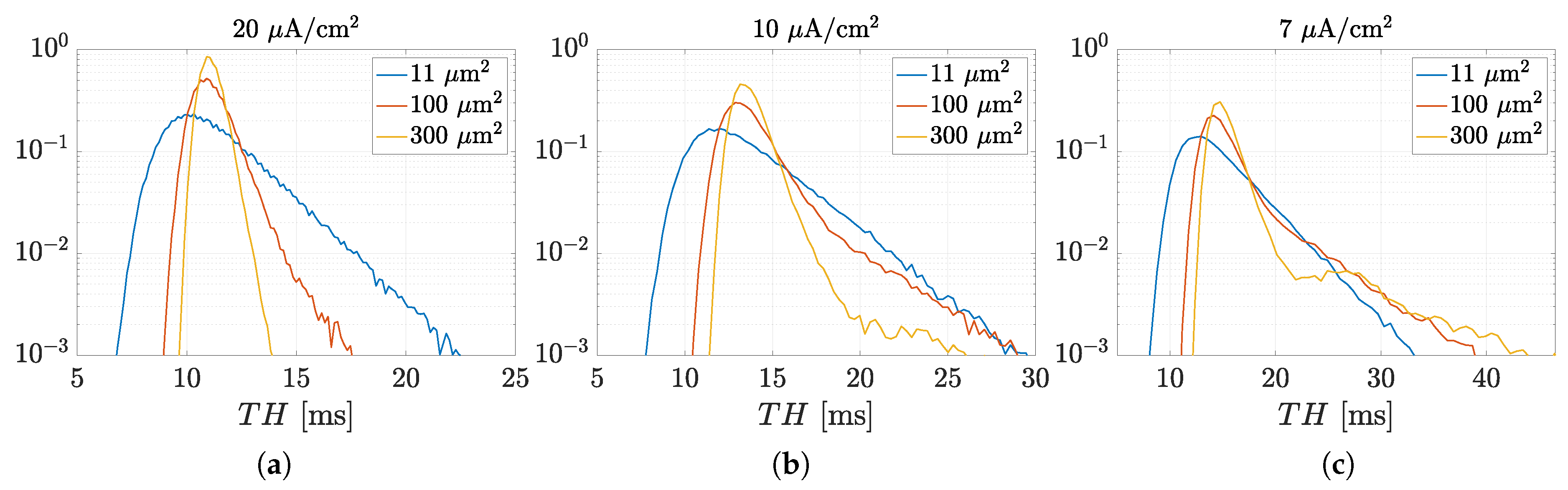
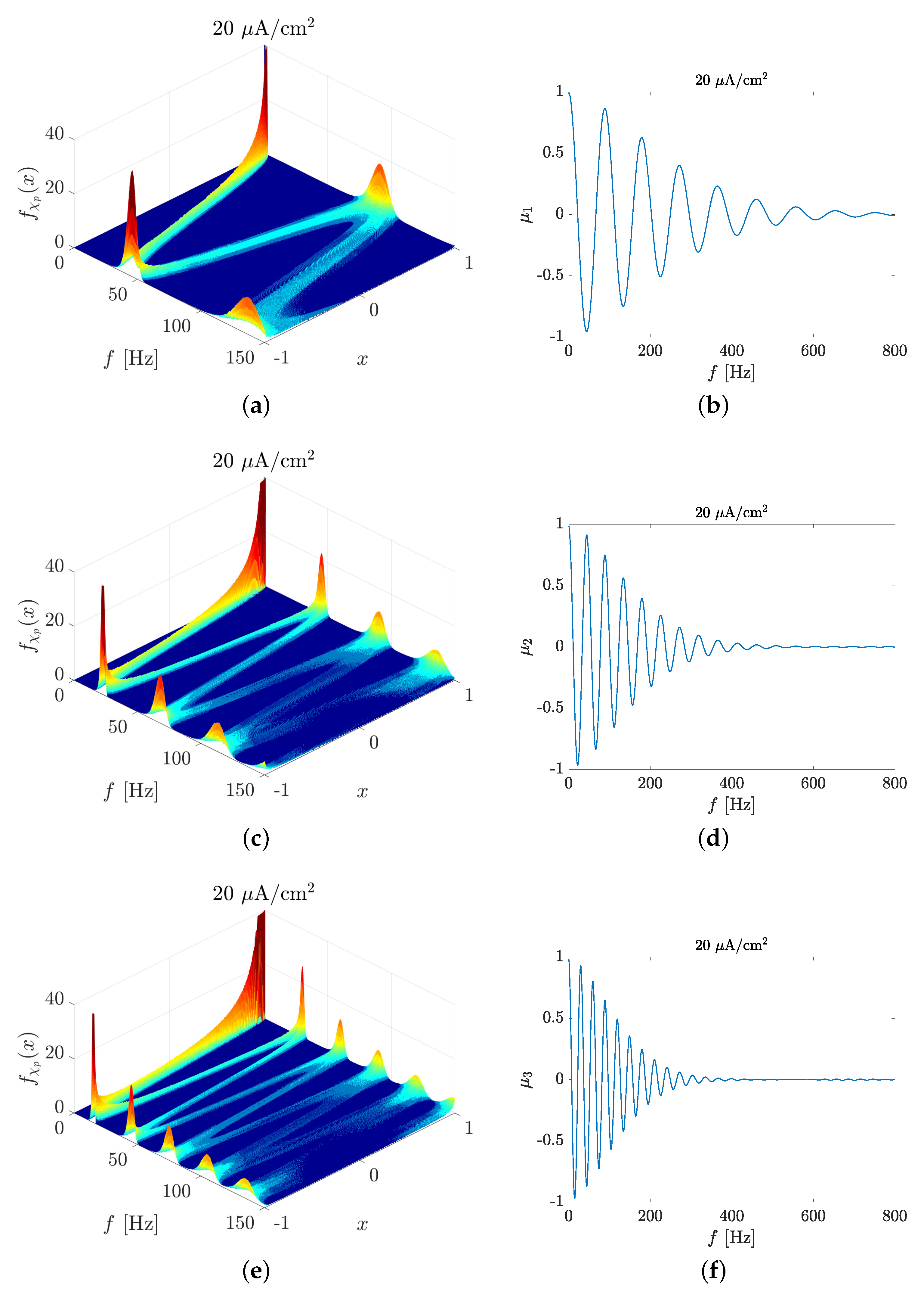
3.1. Spectral Features of Stochastic Neuron Spike Trains

The power spectra, obtained from the simulated spike trains by using the FFT, are shown in Figure 1 for the three current densities: I₀ = 20 μA/cm² (panel a), I₀ = 10 μA/cm² (panel b), I₀ = 7 μA/cm² (panel c). In each panel, spectra obtained for the three patch areas are compared with the deterministic behavior (purple line).

As expected, except for the artifact induced by the spectral leakage, deterministic spectra were a train of pulses centered at the firing frequency and its higher order harmonics. The firing frequency increased with the input current density as reported in literature for an HH neuron model [34]. In the stochastic case, the main peak was not exactly centered at the deterministic firing rate and the other peaks did not correspond to the higher order harmonics of the first one. Moreover, as the frequency increased, they got wider and smaller and shortly disappeared for a high channel noise level, e.g., for the smallest patch area of 11 μm².

Figure 2 shows the differences of peak positions between stochastic and deterministic spectra, for all considered simulation conditions. For patches of 100 μm² and 300 μm² results for the first five peaks are reported in Figure 2, whereas, in the case of 11 μm², only three peaks were faithfully detectable.

Deviation of the main spectral peak from the deterministic firing rate increased with the channel noise and decreased with the input current density, i.e., the more the stochastic behavior prevailed on the deterministic input. It is worth noting that this deviation increased for the higher order peaks, faster and faster as the current density and the patch area decreased.

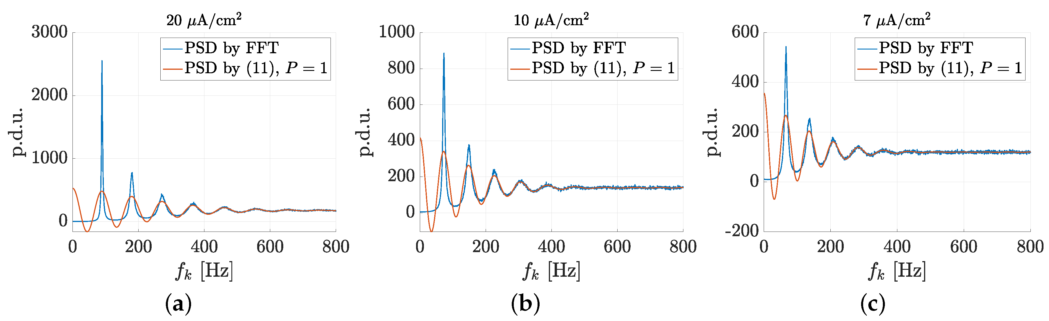
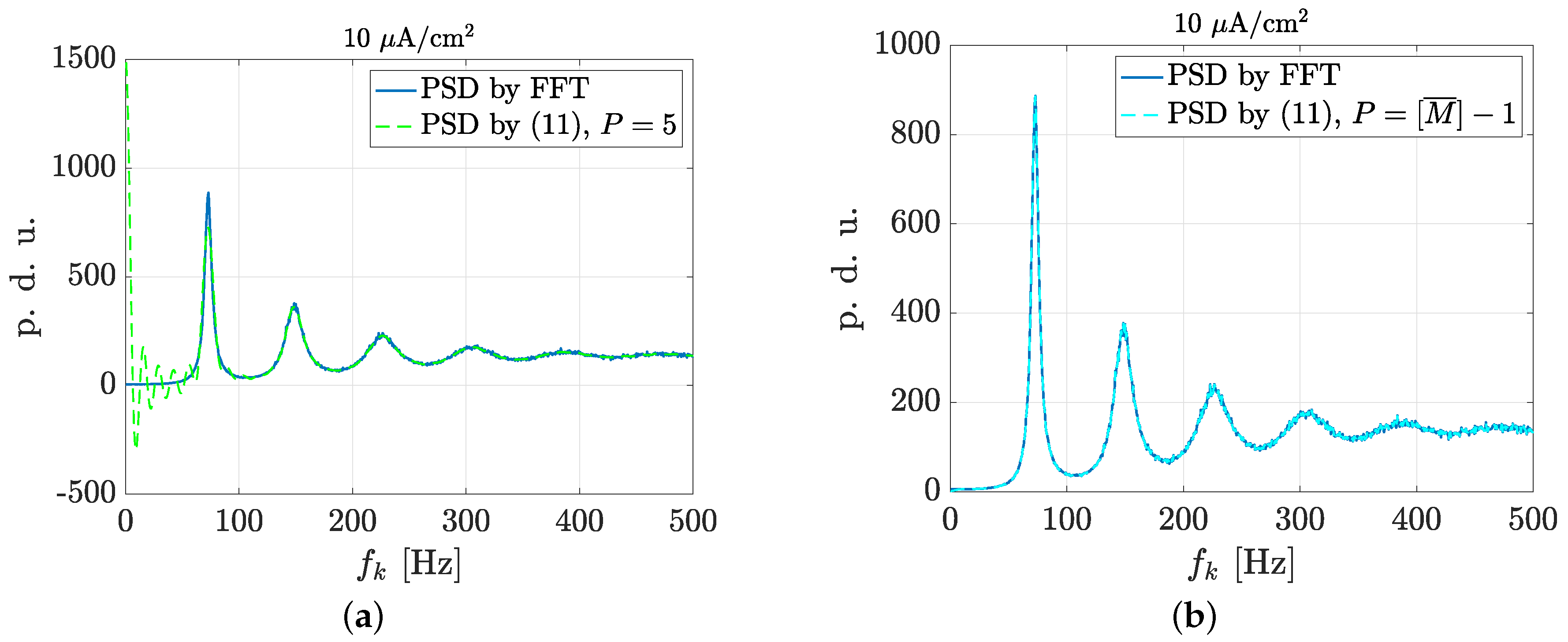
3.2. Estimation of Neuronal Spectral Features

The main results of Section 2.1 (Equation (12)) asserts that the frequency positions of spectral peaks depend on a linear combination of ${\mathsf{\mu }}_p({\omega }_k)$, the mean values of the function ${\chi }_p({\omega }_k)=cosp{\omega }_k\mathsf{\Theta }$. By using the well known formula of the probability density of a non invertible function of random variable, the density of ${\chi }_p({\omega }_k)$ can be written as

$$f_{{\chi }_p}(x)=\sum _{q=1}^{Q_k}\frac{f_{\mathsf{\Theta }}(T{H}_q)}{p{\omega }_k\sqrt{1-x^2}}$$

(13)

where the $T{H}_q$ are the inverse images of x, and the summation is carried out over the $Q_k$ intervals in which the function ${\chi }_p$ is monotone. The expression of $f_{{\chi }_p}(x)$ in (13) shows that it is very difficult to get analytically the trend of ${\mathsf{\mu }}_p(w)$, as well as to connect $f_{\mathsf{\Theta }}$ with the frequencies of spectral peaks. So, in the following, we will investigate this connection starting from the analysis of $f_{\mathsf{\Theta }}(TH)$ and ending to deepen the PSD model (12).

Figure 3 shows the densities $f_{\mathsf{\Theta }}$ per different values of $I_0$: 20 μA/cm² (panel a), 10 μA/cm² (panel b), and 7 μA/cm² (panel c), and three patch areas: 11 μm² (blue lines), 100 μm² (red lines), and 300 μm² (yellow lines). We can notice that for higher $I_0$ values the main peaks were narrower and taller and centered at lower ISI values. Even the patch area affected the ISI distribution: the smaller the area the wider and smaller the main peak, centered at lower ISIs. For $I_0$ = 7 μA/cm² and patch area 300 μm² (yellow line in Figure 3c), the current density was inside the bifurcation range, (6.3–9.8) μA/cm², and a reduced noise level determined the typical multimodal distribution, in line with results presented in [46].

To investigate the relationship between spectral features and the ISI distribution $f_{\mathsf{\Theta }}$, in

Table 1. Frequency of the first peak of Fast Fourier Transform (FFT) ($f_{1\mathrm{PSD}}$), frequency of the first peak of ${\mathsf{\mu }}_1$, mean firing rate, and inverse of interspike interval (ISI) mode.

Current Density	Patch	${\mathit{f}}_{\mathbf{1}\mathbf{PSD}}$	${\mathit{f}}_{\mathbf{1}{\mathsf{\mu }}_{\mathbf{1}}}$	$\mathit{\lambda }$	$\mathbf{1}/\mathbf{mode}\{\mathsf{\Theta }\}$
[$\mathsf{\mu }$A/cm${}^{\mathbf{2}}$]	[$\mathsf{\mu }$m${}^{\mathbf{2}}$]	[Hz]	[Hz]	[Hz]	[Hz]
	11	92.5	90.5	87.9	96.2
20	100	89.5	88.5	88.6	91.0
	300	89.5	89	89.3	91.0
	11	78	76.5	72.1	82.5
10	100	73	72	69.6	76.9
	300	72.5	72	70.7	75.2
	11	73	71	65.4	75.4
7	100	66.5	65.5	59.8	69.2
	300	65	64.5	57.9	66.4

we compared the first peak position in the PSD, $f_{1\mathrm{PSD}}$, with the mean firing rate $\lambda =1/E\{\mathsf{\Theta }\}$[47] and with the inverse of the mode of $\mathsf{\Theta }$.

Looking at Table 1, we can observe that they were almost coincident for the highest current density value (I₀ = 20 μA/cm²) and the highest patch area (300) μm², i.e., when the deterministic behavior dominated. In this case, the frequency of the first peak of ${\mathsf{\mu }}_1$ $f_{1{\mathsf{\mu }}_1}$, the mean firing rate $\lambda$, and $1/\mathrm{mode}\{\mathsf{\Theta }\}$ could all be used as good estimates of the position of the main peak in the spike train spectrum. In the other cases, when the stochastic behavior became more relevant, $\lambda$ underestimated the frequency of the main peak and $1/\mathrm{mode}\{\mathsf{\Theta }\}$ overestimated it.

Except for the simplest case of deterministic models, the frequency of the main peak of the spectrum did not exactly correspond either to the inverse of the mean or the mode of the ISI distribution and the secondary peaks were not centered at multiple frequencies of the main one. Therefore, neuronal spectral features were hardly predictable and interpretable and could not be directly obtained from statistical averages of the ISI distributions.

The PSD model derived in Section 2 allowed us to interpret and evaluate in a very simple and direct way the position of the spectrum peaks.

Equation (12), derived in Section 2, furnishes an approximate model of the PSD of a spike train ($S_u^P[k]$), based on DFT and obtained as a linear combination of ${\mathsf{\mu }}_p({\omega }_k)$, expected value of ${\chi }_p({\omega }_k)$, for $p=1,\dots ,P$.

Figure 4, left column, shows probability density functions of ${\chi }_p({\omega }_k)$, as a function of frequency, for $p=1$ (panel a), $p=2$ (panel c), $p=3$ (panel e), in the case I₀ = 20 μA/cm² and patch area = 100 μm². Panels on the right side of Figure 4 show the expected values of such random variables versus frequency, for the same values of p. As evidenced by looking at panels b, d, and f, ${\mathsf{\mu }}_p({\omega }_k)$ presents cosinusoidal terms which oscillated and decreased faster and faster with frequency as p index increased. As an example, for $p=3$, ${\mathsf{\mu }}_5$ was almost completely damped for f > 300 Hz. Therefore, for high p values, the contribution to the summation of (12) was significant only in the low frequency range. Furthermore the sum of these ${\mathsf{\mu }}_p$, which oscillated faster at low frequencies for high p values, contributed mainly to the almost constant plateau typical of the spike train spectra at lower frequencies than the main peak, whereas at highest frequency tended to zero.

If one considers only the first term ($P=1$) and compares the PSD model $S_u^1[k]=\overline{M}+2(\overline{M}-1){\mathsf{\mu }}_1$ in (12) with the PSD calculated by FFT, as shown in Figure 5 for patch area = 100 μm² and I₀ = 20 μA/cm², 10 μA/cm², and 7 μA/cm², significant differences were evident only in the low frequency range. Indeed, as shown in the Figure 4, in the low frequency range the ${\mathsf{\mu }}_p({\omega }_k)$ with high p were dominant. However, the peak positions almost coincided, as quantitatively shown in

Table 2. Error and mean absolute error between peak frequencies of FFT based PSD and ${\mathsf{\mu }}_1$.

Peaks		1	2	3	4	5
Current Density	Patch	Error					Mean Abs
[$\mathsf{\mu }$A/cm${}^{\mathbf{2}}$]	[$\mathsf{\mu }$m${}^{\mathbf{2}}$]	[Hz]					Error [Hz]
	11	2	0	2.5			1.5
20	100	1	1	0.5	1	1	0.9
	300	0.5	0.5	0.5	1	0.5	0.6
	11	1.5	0.5	−1.5			1.17
10	100	1	1.5	1	0	1.5	1.0
	300	0.5	1.5	1.0	0.5	0.5	0.8
	11	2	1.0	1.5			1.5
7	100	1.0	1.0	0.5	0	1.5	0.8
	300	0.5	1.0	1.0	0.5	0.5	0.7

for all simulated conditions and the first 5 peaks. For the smallest patch area (11 μm²), only the first three peaks were reported as already mentioned in the comment to Figure 2.

Table 2 reports the errors, in terms of difference between peak frequencies of FFT based PSD and ${\mathsf{\mu }}_1$, as well as an average value calculated over all the peaks. It is worth noting that the difference was always below 2 Hz, except for the third peak in the case of the smallest area, i.e., when random fluctuations in the PSD may affect the automatic peak identification. (Looking only at the first peak, which was the most significant from a physiological point of view, the error was equal or lower than 2 Hz, also for the smallest patch).

Therefore, the expected value ${\mathsf{\mu }}_1$ was shown to accurately capture the main frequency components of spike train spectra.

If P increased, $S_u^P[k]$ progressively captured all the shape of the PSD. Figure 6 shows comparison between the FFT based PSD and $S_u^P[k]$ for $P=5$ (panel a) and $P=[\overline{M}]-1$ (panel b), in the case of I₀ = 10 μA/cm² and patch = 100 μm². When summation was limited to the first 5 terms ($P=5$), except for fast oscillations below 60 Hz, the PSD model $S_u^P[k]$ was a good approximation of the FFT spectrum; when all terms of summation were considered ($P=[\overline{M}]-1$), the FFT spectrum was very accurately captured in the whole frequency range.

Furthermore, recalling, with the help of the graphics of ${\mathsf{\mu }}_p({\omega }_k)$ reported in Figure 4, that ${\mathsf{\mu }}_p({\omega }_k)$ tended to zero as frequency increased, the PSD model $S_u^P[k]$ showed that the value of PSD at high frequencies was equal to $\overline{M}$, the square root of the PSD DC value ${\overline{M}}^2$.

4. Conclusions

The PSD of a neuronal spike train has a characteristic shape consisting of peaks and valleys, whose shape and position depend on neuron features and input stimuli. This behavior can be observed in Figure 1, showing the spectra calculated on the outputs of a stochastic HH model where the current density takes into account a deterministic input, whereas the patch area determines the channel noise level. Similar PSD trends were obtained in [24,25] for simple leaky integrate-and-fire (LIF) neurons and in [48] for a sparse recurrent network of LIF neurons driven by stochastic inputs.

When the neuron exhibits a quasi deterministic behaviour, we may consider that the main peak is centered at a frequency equal to the mean firing rate (Figure 3). However, when the stochastic behavior of the neuron becomes significant with respect to the deterministic one, this is no longer true and the characteristic frequencies are difficult to be estimated and interpreted.

Moreover, as evidenced in [49], the detection of spectral peaks in spike trains could be impeded by several biological and experimental factors, so that analytical or semi-analytical approaches are advisable [48,49].

In this work, under the general and well assessed hypothesis that the ISI random variables ${\mathsf{\Theta }}_i$, are i.i.d., we demonstrated that the $S_u^P[k]$, given by (12) can successfully approximate the PSD of neuronal spike trains as shown in Figure 6b, which compares the $S_u^P[k]$ with the PSD numerically calculated using FFT. $S_u^P[k]$ consists of the linear combination of ${\mathsf{\mu }}_p({\omega }_k)$, the expected values of the random variables ${\chi }_p$, $p=1,\dots ,P$. These terms have a damped cosinusoidal trend versus $\omega$ that decays more and more rapidly as p increases. This means that terms corresponding to high p values can be neglected if the exact PSD shape is not needed and that the value of PSD at high frequency is equal to M, the number of spikes in the observation period.

Indeed, the maxima of the first term alone, ${\mathsf{\mu }}_1({\omega }_k)$, are able to estimate the positions of the spectrum peaks with an average error from 0.6 Hz to 1.5 Hz, depending on the model parameters, i.e., the input current density and the membrane patch area and with an absolute error averaged over all simulation conditions equal to 0.94 Hz. This allows us, not only to accurately calculate the frequencies at which the spectral peaks of a spike train are centered, but also to provide a theoretical interpretation of them.

Compared to literature results obtained using PSD analytic formulations on LIF neurons and networks driven by stochastic inputs [24,25,48], our PSDs of the neuronal spontaneous activity exhibit a damped quasi-periodic structure as in [24,48]. Recently, Droste and colleagues [25] showed that the damped PSD structure was strongly related to the features of the considered noise that, in our work, was realistically modeled as the endogenous channel noise. Similarly to the other analytic models present in the literature [24,25,48], even our PSD model gives an exact formulation of the spike-train power spectrum. In addition, it allows us to estimate the PSD features from the ISI statistics, up to the second order, and to give an interpretation of the typical PSD quasi-periodic structure. Indeed, by truncating the expansion of (12) to $p=1$, it is possible an accurate, fast and straightforward calculation of the frequencies corresponding to the main and the higher order spectral peaks. Our PSD model demonstrates that such frequencies do not coincide with the mean firing rate and its multiples, as usually reported in the literature [48].

Although $S_u^P[k]$ has been validated on the ISIs obtained from a stochastic HH neuron model, yet it is applicable to any measured or simulated trace as a quick and accurate estimate of the peak positions. Thus, the simple analytical expression of the proposed PSD model, with respect those available in literature [24,25,48,49], makes it a powerful interpretative tool of PSD shape, also useful for neurophysiological studies aimed at extracting information on neuronal behavior from spike train spectra. Moreover, given the general hypotheses underlying our PSD model, the proposed analysis may be expanded to the outputs of higher levels of biological complexity, such as neuronal networks, and may be applied even to experimental traces recorded through the patch clamp technique or multielectrode array (MEA).

References

1. Johnson, D.H. Point process models of single-neuron discharges. J. Comput. Neurosci. 1996, 3, 275–299. [Google Scholar] [CrossRef]
2. Mino, H. The Effects of Spontaneous Random Activity on Information Transmission in an Auditory Brain Stem Neuron Model. Entropy 2014, 16, 6654–6666. [Google Scholar] [CrossRef] [Green Version]
3. Rinzel, J.; Ermentrout, B. Analysis of neural excitability and oscillations. In Methods in Neuronal Modeling: From Ions to Networks, 2nd ed.; Koch, C., Segev, I., Eds.; MIT Press: Cambridge, MA, USA, 1998; Chapter 7. [Google Scholar]
4. Gammaitoni, L.; Hänggi, P.; Jung, P.; Marchesoni, F. Stochastic resonance. Rev. Mod. Phys. 1998, 70, 223–287. [Google Scholar] [CrossRef]
5. Moss, F. Stochastic resonance and sensory information processing: A tutorial and review of application. Clin. Neurophysiol. 2004, 115, 267–281. [Google Scholar] [CrossRef]
6. Mino, H.; Durand, D.M. Enhancement of information transmission of sub-threshold signals applied to distal positions of dendritic trees in hippocampal CA1 neuron models with stochastic resonance. Biol. Cybern. 2010, 103, 227–236. [Google Scholar] [CrossRef] [PubMed]
7. Bensaid, S.; Modolo, J.; Merlet, I.; Wendling, F.; Benquet, P. COALIA: A Computational Model of Human EEG for Consciousness Research. Front. Syst. Neurosci. 2019, 13. [Google Scholar] [CrossRef] [PubMed]
8. Modolo, J.; Legros, A.; Beuter, A. The next move in neuromodulation therapy: A question of timing. Front. Comput. Neurosci. 2015, 8. [Google Scholar] [CrossRef] [Green Version]
9. Modolo, J.; Legros, A.; Thomas, A.W.; Beuter, A. Model-driven therapeutic treatment of neurological disorders: Reshaping brain rhythms with neuromodulation. Interface Focus 2011, 1, 61–74. [Google Scholar] [CrossRef]
10. Engel, A.K.; Fries, P.; Singer, W. Dynamic predictions: Oscillations and synchrony in top-down processing. Nat. Rev. Neurosci. 2001, 2, 704–716. [Google Scholar] [CrossRef]
11. Hutchison, W.D.; Dostrovsky, J.O.; Walters, J.R.; Courtemanche, R.; Boraud, T.; Goldberg, J.; Brown, P. Neuronal oscillations in the basal ganglia and movement disorders: Evidence from whole animal and human recordings. J. Neurosci. Off. J. Soc. Neurosci. 2004, 24, 9240–9243. [Google Scholar] [CrossRef]
12. Buzsáki, G.; Draguhn, A. Neuronal oscillations in cortical networks. Science 2004, 304, 1926–1929. [Google Scholar] [CrossRef] [PubMed] [Green Version]
13. Czanner, G.; Sarma, S.V.; Ba, D.; Eden, U.T.; Wu, W.; Eskandar, E.; Lim, H.H.; Temereanca, S.; Suzuki, W.A.; Brown, E.N. Measuring the signal-to-noise ratio of a neuron. Proc. Natl. Acad. Sci. USA 2015, 112, 7141–7146. [Google Scholar] [CrossRef] [PubMed] [Green Version]
14. Gray, C.M.; Singer, W. Stimulus-specific neuronal oscillations in orientation columns of cat visual cortex. Proc. Natl. Acad. Sci. USA 1989, 86, 1698–1702. [Google Scholar] [CrossRef] [PubMed] [Green Version]
15. Buzsáki, G. Rhythms of the Brain; Oxford University Press: Oxford, UK, 2006. [Google Scholar] [CrossRef] [Green Version]
16. Jarvis, M.R.; Mitra, P.P. Sampling properties of the spectrum and coherency of sequences of action potentials. Neural Comput. 2001, 13, 717–749. [Google Scholar] [CrossRef] [Green Version]
17. Moran, A.; Bar-Gad, I. Revealing neuronal functional organization through the relation between multi-scale oscillatory extracellular signals. J. Neurosci. Methods 2010. [Google Scholar] [CrossRef] [PubMed]
18. Andres, D.S.; Cerquetti, D.F.; Merello, M. Turbulence in Globus pallidum neurons in patients with Parkinson’s disease: Exponential decay of the power spectrum. J. Neurosci. Methods 2011, 197, 14–20. [Google Scholar] [CrossRef] [PubMed]
19. Mazzoni, A.; Broccard, F.D.; Garcia-Perez, E.; Bonifazi, P.; Ruaro, M.E.; Torre, V. On the Dynamics of the Spontaneous Activity in Neuronal Networks. PLoS ONE 2007, 2, e439. [Google Scholar] [CrossRef] [Green Version]
20. Bédard, C.; Kröger, H.; Destexhe, A. Does the 1/f Frequency Scaling of Brain Signals Reflect Self-Organized Critical States? Phys. Rev. Lett. 2006, 97, 118102. [Google Scholar] [CrossRef] [Green Version]
21. Mitaim, S.; Kosko, B. Adaptive stochastic resonance. Proc. IEEE 1998. [Google Scholar] [CrossRef]
22. Paffi, A.; Camera, F.; Apollonio, F.; D’Inzeo, G.; Liberti, M. Restoring the encoding properties of a stochastic neuron model by an exogenous noise. Front. Comput. Neurosci. 2015, 9, 1–11. [Google Scholar] [CrossRef] [Green Version]
23. Orcioni, S.; Paffi, A.; Camera, F.; Apollonio, F.; Liberti, M. Automatic decoding of input sinusoidal signal in a neuron model: Improved SNR spectrum by low-pass homomorphic filtering. Neurocomputing 2017, 267, 605–614. [Google Scholar] [CrossRef]
24. Lindner, B.; Schimansky-Geier, L.; Longtin, A. Maximizing spike train coherence or incoherence in the leaky integrate-and-fire model. Phys. Rev. E 2002, 66, 031916. [Google Scholar] [CrossRef] [PubMed] [Green Version]
25. Droste, F.; Lindner, B. Exact results for power spectrum and susceptibility of a leaky integrate-and-fire neuron with two-state noise. Phys. Rev. E 2017, 95, 012411. [Google Scholar] [CrossRef] [Green Version]
26. Ozer, M.; Perc, M.; Uzuntarla, M.; Koklukaya, E. Weak signal propagation through noisy feedforward neuronal networks. NeuroReport 2010, 21, 338–343. [Google Scholar] [CrossRef] [PubMed]
27. Paffi, A.; Apollonio, F.; D’Inzeo, G.; Liberti, M. Stochastic resonance induced by exogenous noise in a model of a neuronal network. Netw. Comput. Neural Syst. 2013, 24, 99–113. [Google Scholar] [CrossRef] [PubMed]
28. Goychuk, I.; Hänggi, P. Nonstationary stochastic resonance viewed through the lens of information theory. Eur. Phys. J. B 2009, 69, 29–35. [Google Scholar] [CrossRef] [Green Version]
29. Wiesenfeld, K.; Jaramillo, F. Minireview of stochastic resonance. Chaos Interdiscip. J. Nonlinear Sci. 1998, 8, 539–548. [Google Scholar] [CrossRef]
30. Voronenko, S.O.; Stannat, W.; Lindner, B. Shifting Spike Times or Adding and Deleting Spikes—How Different Types of Noise Shape Signal Transmission in Neural Populations. J. Math. Neurosci. 2015, 5, 1. [Google Scholar] [CrossRef] [Green Version]
31. Orcioni, S.; Paffi, A.; Camera, F.; Apollonio, F.; Liberti, M. Automatic decoding of input sinusoidal signal in a neuron model: High pass homomorphic filtering. Neurocomputing 2018, 292, 165–173. [Google Scholar] [CrossRef]
32. Biagetti, G.; Crippa, P.; Orcioni, S.; Turchetti, C. Homomorphic Deconvolution for MUAP Estimation From Surface EMG Signals. IEEE J. Biomed. Health Informatics 2017, 21, 328–338. [Google Scholar] [CrossRef]
33. Abbott, L. Lapicque’s introduction of the integrate-and-fire model neuron (1907). Brain Res. Bull. 1999, 50, 303–304. [Google Scholar] [CrossRef]
34. Izhikevich, E.M. Dynamical Systems in Neuroscience: The Geometry of Excitability and Bursting; MIT Press: Cambridge, MA, USA, 2005. [Google Scholar]
35. Mainen, Z.; Sejnowski, T. Reliability of spike timing in neocortical neurons. Science 1995, 268, 1503–1506. [Google Scholar] [CrossRef] [PubMed] [Green Version]
36. Halliday, D.M.; Rosenberg, J.R. Time and Frequency Domain Analysis of Spike Train and Time Series Data. In Modern Techniques in Neuroscience Research; Windhorst, U., Johansson, H., Eds.; Springer: Berlin/Heidelberg, Germany, 1999; pp. 503–543. [Google Scholar]
37. Brillinger, D.R. Comparative aspects of the study of ordinary time series and of point processes. In Developments in Statistics; Krishnaiah, P.R., Ed.; Academic Press: Cambridge, MA, USA, 1978; pp. 33–133. [Google Scholar]
38. Wald, A. Some Generalizations of the Theory of Cumulative Sums of Random Variables. Ann. Math. Stat. 1945, 16, 287–293. [Google Scholar] [CrossRef]
39. Rubinstein, J. Threshold fluctuations in an N sodium channel model of the node of Ranvier. Biophys. J. 1995, 68, 779–785. [Google Scholar] [CrossRef] [Green Version]
40. Mino, H.; Rubinstein, J.T.; White, J.A. Comparison of Algorithms for the Simulation of Action Potentials with Stochastic Sodium Channels. Ann. Biomed. Eng. 2002, 30, 578–587. [Google Scholar] [CrossRef] [PubMed]
41. James, F. Monte Carlo theory and practice. Rep. Prog. Phys. 1980, 43, 1145–1189. [Google Scholar] [CrossRef]
42. Izhikevich, E.M. Dynamical Systems in Neuroscience; The MIT Press: Cambridge, MA, USA, 2006. [Google Scholar]
43. Schneidman, E.; Freedman, B.; Segev, I. Ion Channel Stochasticity May Be Critical in Determining the Reliability and Precision of Spike Timing. Neural Comput. 1998, 10, 1679–1703. [Google Scholar] [CrossRef] [Green Version]
44. White, J.A.; Rubinstein, J.T.; Kay, A.R. Channel noise in neurons. Trends Neurosci. 2000, 23, 131–137. [Google Scholar] [CrossRef]
45. Ostrovskii, V.Y.; Karimov, T.I.; Solomevich, E.P.; Kolev, G.Y.; Butusov, D.N. Numerical Effects in Computer Simulation of Simplified Hodgkin-huxley Model. In Proceedings of the 24th International Conference on Oral and Maxillofacial Surgery, ICoMS’19, Rio de Janeiro, Brazil, 21–24 May 2019; ACM Press: New York, NY, USA, 2019; pp. 92–95. [Google Scholar] [CrossRef]
46. Rowat, P.F.; Greenwood, P.E. The ISI distribution of the stochastic Hodgkin-Huxley neuron. Front. Comput. Neurosci. 2014, 8, 111. [Google Scholar] [CrossRef] [Green Version]
47. Kostal, L.; Lansky, P.; Stiber, M. Statistics of inverse interspike intervals: The instantaneous firing rate revisited. Chaos Interdiscip. J. Nonlinear Sci. 2018, 28, 106305. [Google Scholar] [CrossRef] [Green Version]
48. Dummer, B.; Wieland, S.; Lindner, B. Self-consistent determination of the spike-train power spectrum in a neural network with sparse connectivity. Front. Comput. Neurosci. 2014, 8. [Google Scholar] [CrossRef] [PubMed] [Green Version]
49. Matzner, A.; Bar-Gad, I. Quantifying Spike Train Oscillations: Biases, Distortions and Solutions. PLoS Comput. Biol. 2015, 11, e1004252. [Google Scholar] [CrossRef] [PubMed]
Figure 1. Power spectra for I0 = (20, 10, 7) μA/cm2, and patch = (11, 100, 300) μm2.
Mathematics 08 01011 g001
Figure 2. Difference between spectrum peaks of deterministic and stochastic neuron for all currents and patches.
Mathematics 08 01011 g002
Figure 3. Probability densities f Θ ( T H ) for I0 = (20, 10, 7) μA/cm2; and patch = (11, 100, 300) μm2.
Mathematics 08 01011 g003
Figure 4. Probability density of χ p ( ω k ) are shown in panels (a,c,e) for p = 1 , 2, and 3, respectively. μ p , expected value of χ p ( ω k ) , are shown in panels (b,d,f) for p = 1 , 2, and 3, respectively. In all panels I0 = 20 μAcm2, and patch = 100 μm2.
Mathematics 08 01011 g004
Figure 5. Prediction of frequencies of power spectra peaks with μ 1 (red solid line). Panels (ac) report, respectively, power spectra for I0 = (20, 10, 7) μA/cm2, patch = 100 μm2.
Mathematics 08 01011 g005
Figure 6. Comparison of power spectra, for I0 = 10 μA/cm2, patch = 100 μm2, obtained by means of FFT (blue solid line) and (12) with (a) P = 5 (green dashed line) and (b) P = [ M ¯ ] 1 = 138 (cyan dashed line).
Mathematics 08 01011 g006