Article

An Extension of Fuzzy Competition Graph and Its Uses in Manufacturing Industries

by
Tarasankar Pramanik
1,†,
G. Muhiuddin
2,*,†,
Abdulaziz M. Alanazi
2,† and
Madhumangal Pal
3,†
1
Department of Mathematics, Khanpur Gangche High School, Paschim Medinipur 721201, India
2
Department of Mathematics, University of Tabuk, Tabuk 71491, Saudi Arabia
3
Department of Applied Mathematics with Oceanology and Computer Programming, Vidyasagar University, Midnapore 721102, Inida
*
Author to whom correspondence should be addressed.
These authors contributed equally to this work.
Mathematics 2020, 8(6), 1008; https://doi.org/10.3390/math8061008
Submission received: 11 May 2020 / Revised: 5 June 2020 / Accepted: 10 June 2020 / Published: 19 June 2020
(This article belongs to the Special Issue Fuzzy Sets, Fuzzy Logic and Their Applications 2020)

Abstract

:
Competition graph is a graph which constitutes from a directed graph (digraph) with an edge between two vertices if they have some common preys in the digraph. Moreover, Fuzzy competition graph (briefly, FCG) is the higher extension of the crisp competition graph by assigning fuzzy value to each vertex and edge. Also, Interval-valued FCG (briefly, IVFCG) is another higher extension of fuzzy competition graph by taking each fuzzy value as a sub-interval of the interval [ 0 , 1 ] . This graph arises in many real world systems; one of them is discussed as follows: Each and every species in nature basically needs ecological balance to survive. The existing species depends on one another for food. If there happens any extinction of any species, there must be a crisis of food among those species which depend on that extinct species. The height of food crisis among those species varies according to their ecological status, environment and encompassing atmosphere. So, the prey to prey relationship among the species cannot be assessed exactly. Therefore, the assessment of competition of species is vague or shadowy. Motivated from this idea, in this paper IVFCG is introduced and several properties of IVFCG and its two variants interval-valued fuzzy k-competition graphs (briefly, IVFKCG) and interval-valued fuzzy m-step competition graphs (briefly, IVFMCG) are presented. The work is helpful to assess the strength of competition among competitors in the field of competitive network system. Furthermore, homomorphic and isomorphic properties of IVFCG are also discussed. Finally, an appropriate application of IVFCG in the competition among the production companies in market is presented to highlight the relevance of IVFCG.

1. Introduction

Cohen [1] first developed the concept of competition graph (CG) to solve the problem of the food web in ecology. The problem of a food web is to describe the predator-prey relationship among species in the community. Food web is a relationship network framed to describe the relationships among food habits of species. It is a fact that there is a predator-prey relation in ecosystem among the species. The plants are the main source of energy for all the living entity. Species are classified into few levels depending on the predator-prey relationship; for example, primary producer (plants), primary consumer (herbivorous), secondary consumer (carnivorous) and omnivorous. In ecosphere, the plants those are the primary producers can produce through photosynthesis. Herbivorous eats only plants for energy, carnivorous takes herbivorous as their food. There is no unique choice of food to omnivorous. From primary producers to secondary consumers there is a food chain among themselves. But the food web is not same at all as a food chain. An example of a food web is shown in Figure 1. In this figure, grasses are the main source of food and grasshoppers eat them, frogs eat grasshoppers, snakes eat frogs, peacocks have snakes but, eagle depends on snakes as well as grasshoppers. If some species say grasshopper, abolished in this food web, other species (here, eagle) who depend on the abolished species may either exterminate or may have to make every effort for existence adapting another food habit depending on ecological nook, habitat and surrounding atmosphere. Same species may have different food habits in different places depending on ecosystem, habitat and surrounding atmosphere. In this example, shown in Figure 1, it is considered that in a certain ecosystem, 70–80% eagle depends on the grasshopper and 30–40% on snake for his food need. These can be transferred to its similar correspondence to interval-valued fuzzy number as [0.7, 0.8] and [0.3, 0.4] respectively. Peacock has 100% dependence on snake, the snake has 100% dependence on frog and frog has that on a grasshopper. Grasshopper depends only on grass. If any two species depends on the same species, there must be a competition between those two species. Being motivated by this idea, we can model up this natural phenomenon as an IVFCG. In addition to ecology, this graph model has many uses in circuit designing, economical model and coding as well as energy systems, etc.
We have generalized the model to its more realistic cases as an IVFCG. In IVFCG, the vertices and edges may be considered as an interval of numbers instead of precise numbers.
Graph theory has an extensive sector of applications in the real world. In 1975, Rosenfeld [2] generalizes the Euler’s graph theory model to fuzzy graph (briefly, FG) theory. Before generalizing graph theory, he has studied the fuzzy relation (briefly, FR) of fuzzy sets and he also introduced several types of FGs. The scope of FG theory is widening fast for its demand in society. The FG theory is being extensively used to solve the problems on the system where there is a network which is either physical, biological or artificial such as, the neuron in the human brain, rail routing system, transportation problem, traffic signaling system, scheduling problem, etc. In the fuzzy field of mathematics, there are various types of FGs which are classified as follows:
  • the set of all vertices is crisp and the set of all edges is fuzzy
  • the set of all vertices is fuzzy and the set of all edges is crisp
  • the set of all vertices is fuzzy and the set of all edges is fuzzy
  • the sets of all vertices and edges are crisp with fuzzy connectivity.
Among these, the most studied type of FGs is the third one, as this is the more general case of FGs. Fuzzy systems are applied to the problems where approximate reasoning is involved.
A fuzzy set (FS) δ is a pair δ = ( S , δ ) the membership function (MF) δ : S [ 0 , 1 ] where S is a vertex set. There are different types of FSs which are extended further such as BFS, interval-valued FS (IVFS), intuitionistic FS, etc.
Zadeh [3] developed the concept of IVFSs as a generalization of FSs in which the membership values lies in [ 0 , 1 ] instead of a precise number. Since the IVFS is an interval number, it is more strong enough to consider real-world problems than the traditional FSs. Therefore, it has more area of applications such as medical diagnosis, multivalued logic, fuzzy control, approximate reasoning, intelligent control, etc.

1.1. Motivation and Main Contribution of the Proposed Work

As we have seen, there is competition in most of our real-world problem, especially in industries, ecology, or wherever the economy is involved. This competition depends on certain parameters. These parameters can be anything like time, money, demand, etc. In the case of competitive real-world problems, the contestant has to accurately determine who his competitors are and how strong they are. In a system where many competitors are related to each other in different ways, it is possible to make this diagnosis accurately with the help of a mathematical model. But one thing to note about these parameters is that their values are never specified in the case of real-world problems. Time is an important parameter when marketing a product in such a market industry. But in this case, it is very true that no one can say in advance exactly when a product can be marketed. It can be said that the product can be marketed at any time interval like 1 to 2 months or 30 days to 45 days, etc. Due to this kind of vagueness in the quality of parameters, we will use fuzzy mathematical model instead of using any crisp mathematical model. However, the simple fuzzy set system is multi-valued but cannot express the idea of the ‘interval’ properly. So in this paper, we have proposed to extend our existing fuzzy system to an interval-valued fuzzy system in competition graph model.
Main contribution of the proposed work is to find the strength of competition among competitors exists in a network so that the competitors can decide their strong competitors and take positive steps to achieve its profit. IVFCG is useful rather than other methods because:
  • most of real-world problems are those networks whose nodes have vague parameters and this method deal with such type of networks well.
  • if the parameters associated with the nodes of the networks are of interval then the method is very much useful in dealing such.
  • an efficient algorithmic approach.
Authors’ contribution towards the development of interval-valued fuzzy competition graph and making use of it in market competition is listed in Table 1.

1.2. Review of Previous Works

To represent any network in the mathematical model we use graphs. The graph is dealt with several physical, biological, social, economic relationships very well. For example, friendship is a social relationship network which is modelled as a graph for several community sites such as Facebook, Twitter, LinkedIn, etc. in many forms and they have several problems to solve related to this network. In the cases where the impreciseness in relations comes, the corresponding relationship network can be modelled as an FG model. In 2003, Bhutani and Battou [11] consider the operations on FGs where the m-strong property is reserved. The necessity of finding strongness in FGs demands the contribution of Bhutani and Rosenfeld [12] to find strong arcs in FGs. The reader may look for more characterization of FGs in [13,14].
There are a lot of variations in CGs described in Cohen’s work [1]. Several researchers have found various derivations of competition graphs. Such as Cho et al. [6] developed the m-step CG of a digraph. The p-CG of a digraph has been defined by Kim et al. [4,15]. The tolerance CG is defined by Brigham et al. [5]. The competition hypergraphs have been found in Sonnatag et al. [7]. Recent work on FKCG and p-competition FGs is available in [8]. Nayeem and Pal [16] have worked to find the shortest path in a network where the relationship between the nodes is imprecise. A detailed survey of the works on CG can be found in [17]. Recently, the fuzzy tolerance graph [18] is further extended to fuzzy ϕ -tolerance CG by Pramanik et al. [9]. To emphasize real-world problem Samanta and Pal [19,20] have studied fuzzy planar graph. Pramanik et al. [21] have generalized the fuzzy planar graph by introducing the IVFSs instead of traditional FSs. Rashmanlou and Pal [22] have studied several properties on highly irregular interval-valued FGs (IVFG). To find the shortest path in a complex network is very emerging work in this modern edge. There are various techniques to find shortest paths in a network. The bipolar fuzzy hypergraph is an extension of fuzzy hypergraph by introducing bipolar fuzzy vertex sets (or simply, bipolar FS (BFS)) and bipolar FR instead of traditional FSs. The bipolar FG (BFG) is introduced by Samanta and Pal [23] which has emerging importance in a complex networking system. Colouring problem is also a challenging task in the research field nowadays. Samanta et al. [24] have introduced a new approach to colour an FG in a vague sense. Rashmanlou et al. [25] have worked on bipolar fuzzy graphs which is an extension of fuzzy graphs. In 2014, Rashmanlou and Pal [26] have studied the properties of isometry on interval-valued fuzzy graphs. Balanced interval-valued fuzzy graphs [27] and Antipodal interval-valued fuzzy graphs [28] are another two types of fuzzy graphs which are introduced by Rashmanlou and Pal. For further studies on FGs and its variations the works of literature [29,30,31] may be very helpful.
There may occur challenging situations in a system’s operation characterized by a degree of vagueness and/or uncertainty. Voskoglou [32] uses principles of fuzzy logic to develop a general model representing such kind of situations. He also introduced a stochastic method for the description of a finite Markov chain as the main steps of mathematical modelling process in [33]. In 2012, a fuzzy model [34] has been developed by him to describe the process of Analogical Reasoning. Gil et al. [35] have determined the travel and delay times in a road ending in a traffic light under different traffic flows and traffic light cycles using a microscopic traffic simulator. To find the approximate measure of the behavior of the plant Hedrea et al. [36] uses TP-based model transformation method in order to obtain a Tensor Product-based model of magnetic levitation systems. Deveci et al. [37] developed a quantitative assessment framework for public bus operators to translate the passenger demands into service quality specifications. Recently, Deveci et al. [38] have developed a multi-criteria decision-making model considering technical, economic, environmental and social criteria to assess Ireland’s most promising offshore wind sites. In airlines, crew scheduling problem is a challenging problem. Deveci and Demirel have proposed a solution and made a survey on this in [39]. Canitez and Deveci [40] have presented a model framework so that public transport system and multi-stakeholder can better manage car sharing applications. In 2015, Deveci et al. [41] studied fuzzy-based multi-criteria decision making methods to solve the carbon di-oxide geological storage location selection problem.
In this paper, IVFCG is defined and investigated several properties on this graph. Also, several variations of this graph class such as interval-valued m-step FCG, IVFKCG, etc. are introduced. The homomorphism and isomorphism properties of several IVFCG products have also been studied. An application on the competition of producers for their products is discussed. This application and the application on ecosystem discussed earlier shows the importance of IVFCG.
The arrangements for the paper are as follows:
After a short inception in Section 1, previous works have been reviewed in Section 1.2. In Section 2, the needful preliminaries that have been surveyed are placed. The main work of IVFCG is introduced in Section 3. Introducing Definition of IVFCG, many results have been studied there. Section 4 describes an interesting idea to apply in the real field. Homomorphism properties of IVFG products have been studied in Section 5. Next, the conclusion has been drawn in Section 6.

2. Preliminaries

A FS δ on a set S is a function δ : S [ 0 , 1 ] , known as the MF. The support of δ is supp ( δ ) = { d S | δ ( d ) 0 } and the core of δ is core ( δ ) = { d S | δ ( d ) = 1 } . The support length is s ( δ ) = | supp ( δ ) | and the core length is c ( δ ) = | core ( δ ) | . The height of δ is h ( δ ) = max { δ ( d ) | d S } . The FS δ is said to be normal if h ( δ ) = 1 .
A FG is defined on a non-empty finite set S equipped with FS δ defined by a MF δ : S [ 0 , 1 ] and a FR θ on the FS δ such that θ ( p , q ) δ ( p ) δ ( q ) for all p , q S , where ∧ represents minimum. A fuzzy edge ( p , q ) , p , q S is said to be independent strong [31] if θ ( p , q ) 1 2 min { δ ( p ) , δ ( q ) } and is called weak, otherwise. The degree of a vertex d of a FG G = ( S , δ , θ ) is d e g ( d ) = c S { d } θ ( d , c ) . The order of a FG G is O ( G ) = c S δ ( c ) . The size [22] of a FG G is S ( G ) = θ ( c , d ) .
A directed FG or, fuzzy digraph (FDG) [42] F = ( S , δ , ν ) defined on a non-empty set S equipped with a fuzzy MF δ : S [ 0 , 1 ] and a FR ν : S × S [ 0 , 1 ] such that for all c , d S , ν ( c , d ) δ ( c ) δ ( d ) .
As ν need not be symmetric, an FDG may consists of two directed edges between two vertices with opposite directions. These edges are called parallel edges. There exists a loop at a vertex c S , if ν ( c , c ) 0 .
Every FG corresponds to an undirected FG F = ( S , δ , θ ) where θ ( c , d ) = max { ν ( c , d ) , ν ( d , c ) } c , d S and this undirected FG is called the underlying FG [31].
A complete FDG is an FDG F = ( S , δ , ν ) in which the relation ν ( c , d ) = ν ( d , c ) = δ ( c ) δ ( d ) for all c , d S holds.
To introduce the CG, Cohen defined a digraph F = ( S , E ) which nicely represents an ecological problem of food web. In food web, species are represented as vertex p in S ( F ) and an arc ( p , s ) in E ( F ) means that p preys on species s. A vertex p S ( F ) represents a species in the food web and arc ( p , s ) E ( F ) means that p is dependent on the species s. If a prey s is dependent on two different species then it is said that the two species compete for the prey s. Therefore, each species in the food web are interdependent and this interdependence is designed by Cohen as competition graph model. An undirected graph G = ( S , E ) of a digraph F = ( S , E ) with same vertex set S is said to be CG if between any two vertices p , q there is an edge in E, such that the arcs ( p , s ) , ( q , s ) are in E ( F ) . Several fields like channel assignment, energy systems, modeling of complex economic, coding, etc. uses the study of CG.
In an FDG F = ( S , δ , ν ) , the fuzzy out-neighbourhood [31] of a vertex d S is a FS Δ + ( d ) = ( S v + , m v + ) , where S v + = { c | ν ( d , c ) > 0 } and m v + : S v + [ 0 , 1 ] is defined by m v + = ν ( d , c ) .
In an FDG F = ( S , δ , ν ) , the fuzzy in-neighbourhood [31] of a vertex d S is a FS Δ ( d ) = ( S v , m v ) , where S v = { c | ν ( c , d ) > 0 } and m v : S v [ 0 , 1 ] is defined by m v = ν ( c , d ) .
In a FG F = ( S , δ , θ ) , the fuzzy neighbourhood [43] of a vertex d S is the FS Δ ( d ) = ( S v , m v ) , where S v = { c | θ ( c , d ) > 0 } and m v : S v [ 0 , 1 ] is defined by m v = θ ( c , d ) .
A FS Δ m + ( d ) = ( S v + , m v + ) , where S v + = { c | θ m ( d , c ) = min { ν ( d , c 1 ) , ν ( c 1 , c 2 ) , , ν ( c m , c ) } > 0 , v c 1 c 2 c m c is a path from d to c } and m v + : X v + [ 0 , 1 ] is said to be the m-step fuzzy out-neighbourhood [31] of a vertex d S of a directed FG F = ( S , δ , ν ) .
The FCG [31] of an FDG F = ( S , δ , ν ) is an undirected graph C ( F ) = ( S , δ , θ ) which has the same fuzzy vertex set as in F and has a fuzzy edge between two vertices c , d S in C ( F ) if and only if Δ + ( c ) Δ + ( d ) is non-empty FS in F . The membership value of the edge ( c , d ) in C ( F ) is θ ( c , d ) = ( δ ( c ) δ ( d ) ) h ( Δ + ( c ) Δ + ( d ) ) .
The m-step FCG [31] of an FDG F = ( S , δ , ν ) is denoted by C m ( F ) and is defined by C m ( F ) = ( S , δ , θ ) where θ ( c , d ) = ( δ ( c ) δ ( d ) ) h ( Δ m + ( c ) Δ m + ( d ) ) for all c , d S .
An interval number [44] L is an interval [ l , l + ] with 0 l l + 1 . For any two interval numbers L 1 = [ l 1 , l 1 + ] and L 2 = [ l 2 , l 2 + ] the followings are defined:
  • L 1 + L 2 = [ l 1 , l 1 + ] + [ l 2 , l 2 + ] = [ l 1 + l 2 l 1 · l 2 , l 1 + + l 2 + l 1 + · l 2 + ] ,
  • min { L 1 , L 2 } = [ min { l 1 , l 2 } , min { l 1 + , l 2 + } ] ,
  • max { L 1 , L 2 } = [ max { l 1 , l 2 } , max { l 1 + , l 2 + } ] ,
  • L 1 L 2 l 1 l 2 and l 1 + l 2 + ,
  • L 1 = L 2 l 1 = l 2 and l 1 + = l 2 + ,
  • L 1 < L 2 L 1 L 2 but L 1 L 2 ,
  • k L 1 = [ k l 1 , k l 2 + ] , where 0 k 1 .

2.1. Some Terminology of FGs

The fuzzy subgraph [45] of a FG F = ( S , δ , θ ) is a FG F = ( S , τ , ν ) with τ ( c ) δ ( c ) for all c S and ν ( c , d ) θ ( c , d ) for all c , d S .
Definition 1.
A FG F = ( S , δ , θ ) is said to be complete if θ ( c , d ) = min { δ ( c ) , δ ( d ) } for all c , d S .
Strong edge in a FG is defined in many ways in various literature. Among them the definition stated in [46] is more suitable for our purpose. We use this definition in our work too.
Definition 2.
A FG F = ( S , δ , θ ) is called the bipartite FG if there are two non-empty vertex sets S 1 and S 2 such that θ ( d 1 , d 2 ) = 0 if d 1 , d 2 S 1 or d 1 , d 2 S 2 . Further, if θ ( d 1 , d 2 ) = min { δ ( d 1 ) , δ ( d 2 ) } for all d 1 S 1 and d 2 S 2 , then F is called a complete bipartite FG.
An effective edge [47] in a FG F = ( S , δ , θ ) is an edge ( c , d ) such that the condition θ ( c , d ) = min { δ ( c ) , δ ( d ) } holds. The end vertices of the effective edge are called effective adjacent vertices. The number of effective incident edges on a vertex d of a FG is the effective incident degree of the FG. A FG is a complete FG if its all the edges are effective incident. The effective incident degree of a pendent vertex in a FG is defined as 1. If one end vertex of a fuzzy edge of a FG is fuzzy pendent vertex then the fuzzy edge is call fuzzy pendent edge [8]. The membership value of the fuzzy pendent edge is the minimum among the membership values of the fuzzy end vertices.
If the degree of a vertex d of a FG F = ( S , δ , θ ) is a fixed positive real number, say, k for all d S then the FG F is said to be regular [48]. The FG F is called totally regular FG [48] if each vertex of F has same total degree k. If in a FG F there are at least two vertices which are adjacent with distinct degrees, the FG is said to be irregular [49]. If every two adjacent vertices of the FG have different degrees then the FG is said to be neighbourly irregular [49]. If there are at least two adjacent vertices which have distinct total degrees, is said to be totally irregular. The FG is said to be neighbourly total irregular [49] if every two adjacent vertices have distinct total degrees. A FG is said to be highly irregular [49] if every vertex of G is adjacent to vertices with distinct degrees.
Definition 3.
The crisp graph F * = ( S , δ * , θ * ) corresponding to a FG F = ( S , δ , θ ) with same vertex set and δ * = { c S | δ ( c ) > 0 } and θ * = { ( c , d ) S × S | θ ( c , d ) > 0 } is called the underlying crisp graph of the FG F.
The complement [45] of FG F = ( S , δ , θ ) is the FG F = ( S , δ , θ ) where δ ( c ) = δ ( c ) for all c S and
θ ( c , d ) = 0 , if   θ ( c , d ) > 0 , δ ( c ) δ ( d ) , otherwise .
Definition 4
([50]). Let δ be a FS defined by δ : S [ 0 , 1 ] and θ is a FR where θ : S × S [ 0 , 1 ] such that for all c , d S , θ ( c , d ) δ ( c ) δ ( d ) . Then F = ( S , δ , θ ) is said to be an FDG.
Since θ is well defined, an FDG does not have more than two directed edges with opposite directions between any two vertices. The membership value of a directed edge ( c , d ) is denoted by θ ( c , d ) . The loop at a vertex c is mathematically expressed as θ ( c , c ) 0 . Since, in an FDG θ ( c , d ) and θ ( d , c ) may have different values, θ . The underlying crisp graph of FDG is the graph similarly obtained except the directed arcs are replaced by undirected edges.

2.2. Fuzzy Hypergraphs

Goetschel [51] introduced fuzzy hypergraphs. The Definition of fuzzy hypergraph is given below
Definition 5.
Let S be a non-empty finite set and let E be a finite family of nontrivial FSs on S (or subsets of S) such that S = { supp ( A ) | A E }. Then the pair H = ( S , E ) is a fuzzy hypergraph on S.
S and E are respectively vertex set and fuzzy edge set of H . The height of H , h ( H ) , is defined by h ( H ) = m a x { h ( A ) | A E }. A fuzzy hypergraph is simple if E has no repeated fuzzy edges and whenever A , B E and A B , then A = B . A fuzzy hypergraph H = ( S , E ) is support simple if whenever A , B E , A B and s u p p ( A ) = s u p p ( B ) , then A = B . Suppose A = ( X 1 , θ ) F , X 1 S and c ( 0 , 1 ] . The c cut of A, A c , is defined by A c = { c S | θ ( c ) c } . If E c = { A c | E / { ϕ } } and S c = { A c | A E }. If E c ϕ , then the (crisp) hypergraph H c = ( S c , E c ) is the c level hypergraph of H .
Suppose H 1 = ( S , E 1 ) and H 2 = ( S , E 2 ) are fuzzy hypergraphs. Then H 1 is partial hypergraph of H 2 if E 1 E 2 . A FS A = ( S , θ ) with θ : S [ 0 , 1 ] is an elementary FS if θ is constant function or θ has range { 0 , a } , 0 a . An elementary fuzzy hypergraph is a fuzzy hypergraph in which all fuzzy edges are elementary.
A fuzzy hypergraph H = ( S , E ) is a m tempered fuzzy hypergraph of a crisp hypergraph H * = ( S , E ) if there exists a FS A = ( S , m ) such that m : S ( 0 , 1 ] and E = { θ E i | E i E } where
θ E i ( c ) = m i n { m ( e ) | e E i } if   c E i 0 , o t h e r w i s e
A fuzzy transversal T = ( S , τ ) of H is a FS defined on S with the property that τ h ( A ) θ h ( A ) ϕ for each A E (recall that h ( A ) is the height of A). A minimal fuzzy transversal T for H is a transversal of H with the property that if T 1 < T , then T 1 is not a fuzzy transversal of H .

2.3. Fuzzy Intersection Graphs

McAllister [52] introduced fuzzy intersection graphs. The Definition of fuzzy intersection graph is now given.
Definition 6.
F = { A 1 = ( S , m 1 ) , A 2 = ( S , m 2 ) , A n = ( S , m n ) } be a finite family of FSs defined on a set S and consider F as crisp vertex set S = { d 1 , d 2 , v n } . The fuzzy intersection graph of F is the FG I n t ( F ) = ( S , δ , θ ) where δ : S [ 0 , 1 ] is defined by δ ( v i ) = h ( A i ) and θ : S × S [ 0 , 1 ] is defined by
θ ( v i , v j ) = h ( A i A j ) , i f   l j 0 , i f   l = j .

2.4. Bipolar FGs

There are several real relationship network system, where each nodes or relation between them simultaneously have some properties and as well as have opposite properties. For example, in almost every social networking system a member may have two or more properties among them there are two properties are very opposite to each other. Any member of the system may ‘like’ some other member or he may ‘dislike’ the member. This concept introduces a new generalised FS which is called BFS system. The elements of the set have some positive membership values and some negative membership values. Zhang [53], first introduced the concept of BFS as a generalisation of FS. For example, set of all foods constitutes a set with the property ‘sweetness of food’, then this set must be a FS. This property indicates there must have another property ‘bitterness of food’ which also should be traced out. Positive membership values and negative membership values are set by defining grade of sweetness and grade of bitterness of food respectively. Other tastes like salty, sour, pungent (e.g., chili), etc. are irrelevant to the corresponding property. So membership values of tastes of these foods are taken as zero.
The Definition of BFS is given as follows. Let S be a nonempty set. A BFS T on S is an object having the form T = { ( c , m + ( c ) , m ( c ) ) | c S } , where m + : S [ 0 , 1 ] and m : S [ 1 , 0 ] are mappings. If m + ( c ) 0 and m ( c ) = 0 , then we say that c has only the positive satisfaction for T. Similarly, if m + ( c ) = 0 and m ( c ) 0 , it is to be said that the vertex c somewhat satisfies the counter property of T. There may have possibility that a vertex c with m + ( c ) 0 and m ( c ) 0 may satisfy MF so that some its properties overlaps that of its counter property over some portion of S. For the BFS T = { ( c , m + ( c ) , m ( c ) ) | c S } , we simply write T = ( m + , m ) .
For every two BFSs L = ( m L + , m L ) and T = ( m J + , m J ) on S,
( L T ) ( c ) = ( m i n ( m L + ( c ) , m J + ( c ) ) , m a x ( m L ( c ) , m J ( c ) ) ) .
( L T ) ( c ) = ( m a x ( m L + ( c ) , m J + ( c ) ) , m i n ( m L ( c ) , m J ( c ) ) ) .
Akram [44,54] introduced BFGs and investigated some properties of it. The formal Definition is given as follows.
Definition 7.
A BFG on a set S is the pair B = ( L , T ) where L = ( m L + , m L ) is a BFS on S and T = ( m J + , m J ) is a BFS on E S × S such that m J + ( c , q ) min { m L + ( c ) , m L + ( q ) } and m J ( c , q ) max { m L ( c ) , m L ( q ) } for all ( c , q ) E . Here L is called bipolar fuzzy vertex set of S, T is the bipolar fuzzy edge set of E. Thus B = ( L , T ) is a BFG.
A BFG B = ( L , T ) is said to be strong if
m J + ( c , q ) = m i n ( m L + ( c ) , m L + ( q ) ) and m ( c , q ) = m a x ( m L ( c ) , m L ( q ) ) .
The Definition of strong BFG is given below.
Definition 8.
The complement [44] of a strong BFG B is B ¯ = ( L ¯ , T ¯ ) where L ¯ = ( m ¯ L + , m ¯ L ) is a BFS on S ¯ and T ¯ = ( m ¯ J + , m ¯ J ) is a BFS on E ¯ S ¯ × S ¯ such that
(1) S ¯ = S ,
(2) m ¯ L + ( c ) = m L + ( c ) and m ¯ L ( c ) = m L ( c ) for all c S ,
(3)
m ¯ J + ( c , q ) = 0 , i f   m J + ( c , q ) > 0 , m L + ( c ) m L + ( q ) , o t h e r w i s e .
m ¯ J ( c , q ) = 0 , i f   m J ( c , q ) < 0 , m L ( c ) m L ( q ) , o t h e r w i s e .
Definition 9
([44]). Let F = ( L , T ) be a BFG where L = ( m 1 + , m 1 ) and T = ( m 2 + , m 2 ) be two BFSs on a non-empty finite set S and E S × S respectively. The graph F is called complete BFG if m 2 + ( c , d ) = min { m 1 + ( c ) , m 1 + ( d ) } and m 2 ( c , d ) = max { m 1 ( c ) , m 1 ( d ) } for all c , d S .
Regular BFGs are also important subclass of BFGs.
Definition 10
([55]). Let F = ( L , T ) be a BFG where L = ( m 1 + , m 1 ) and T = ( m 2 + , m 2 ) be two BFSs on a non-empty finite set S and E S × S respectively. If d + ( c ) = k 1 , d ( c ) = k 2 for all c S , k 1 , k 2 are two real numbers, then the graph is called ( k 1 , k 2 ) -regular BFG.
Definition 11
([55]). Let F = ( L , T ) be a BFG where L = ( m 1 + , m 1 ) and T = ( m 2 + , m 2 ) be two BFSs on a non-empty finite set S and E S × S respectively. t d ( c ) = ( t d + ( c ) , t d ( c ) ) is the total degree of a vertex c S where t d + ( c ) = ( c , d ) E m 2 + ( c , d ) + m 1 + ( c ) , t d ( c ) = ( c , d ) E m 2 ( c , d ) + m 1 ( c ) . If all the vertices of a BFG are of total degree, then the graph is called totally regular BFG.
An IVFS L on a set S is a mapping θ L : S [ 0 , 1 ] × [ 0 , 1 ] , called the MF, i.e., θ L ( c ) = [ θ L ( c ) , θ L + ( c ) ] . The support of L is supp ( L ) = { c S | θ L ( c ) 0 } and the core of L is core ( L ) = { c S | θ L ( c ) = 1 } . The support length is s ( L ) = | supp ( L ) | and the core length is c ( L ) = | core ( L ) | . The height of L is h ( L ) = max { θ L ( c ) | c S } = [ h ( L ) , h + ( L ) ] = [ max { θ L ( c ) } , max { θ L + ( c ) } ] , c S .
Let F = { L 1 , L 2 , , L n } be a finite family of interval-valued fuzzy subsets on a set S. The fuzzy intersection of two IVFSs (IVFSs) L 1 and L 2 is an IVFS defined by
L 1 L 2 = c , min { θ L 1 ( c ) , θ L 2 ( c ) } , min { θ L 1 + ( c ) , θ L 2 + ( c ) } : c S
The fuzzy union of two IVFSs L 1 and L 2 is a IVFS defined by
L 1 L 2 = c , max { θ L 1 ( c ) , θ L 2 ( c ) } , max { θ L 1 + ( c ) , θ L 2 + ( c ) } : c S
Fuzzy out-neighbourhood of a vertex d S of an interval-valued fuzzy directed graph (IVFDG) F = ( S , L , T ) is the IVFS Δ + ( d ) = ( X v + , m v + ) where X v + = { c : θ T ( d , c ) > 0 } and m v + : X v + [ 0 , 1 ] × [ 0 , 1 ] defined by m v + = θ T ( d , c ) = [ θ T ( d , c ) , θ T + ( d , c ) ]
Here T is an interval-valued FR on a set S, is denoted by θ T : S × S [ 0 , 1 ] × [ 0 , 1 ] such that
θ T ( c , q ) min { θ L ( c ) , θ L ( q ) } θ T + ( c , q ) min { θ L + ( c ) , θ L + ( q ) }
Consider L = [ θ L , θ L + ] is an IVFS on S and T = [ θ T , θ T + ] is an IVFS on S × S then the triplet F = ( S , L , T ) is said to be an IVFG. An edge ( c , d ) , c , d S in an IVFG is said to be independent strong if θ T ( c , d ) 1 2 min { θ L ( c ) , θ L ( d ) } . An interval-valued FDG (IVFDG) F = ( S , L , T ) is an IVFG where the FR T is antisymmetric.
An IVFG Z = ( S , L , T ) is said to be complete IVFG if θ ( c , d ) = min { δ ( c ) , δ ( d ) } and θ + ( c , d ) = min { δ + ( c ) , δ + ( d ) } , c , d S . An IVFG is said to be bipartite if there are two vertex sets S 1 and S 2 such that S 1 S 2 = S and S 1 S 2 = ϕ where θ + ( d 1 , d 2 ) = 0 if d 1 , d 2 S 1 or d 1 , d 2 S 2 and θ + ( d 1 , d 2 ) > 0 if d 1 S 1 (or S 2 ) and d 2 S 2 (or S 1 ).
The Cartesian product [44] Z 1 × Z 2 of two IVFGs Z 1 = ( S 1 , L 1 , T 1 ) and Z 2 = ( S 2 , L 2 , T 2 ) is defined as a pair ( S 1 × S 2 , L 1 × L 2 , T 1 × T 2 ) such that
  • θ L 1 × L 2 ( p 1 , p 2 ) = min { θ L 1 ( p 1 ) , θ L 2 ( p 2 ) } θ L 1 × L 2 + ( p 1 , p 2 ) = min { θ L 1 + ( p 1 ) , θ L 2 + ( p 2 ) } ,
    for all p 1 S 1 , p 2 S 2 ,
  • θ T 1 × T 2 ( ( c , p 2 ) , ( c , q 2 ) ) = min { θ L 1 ( c ) , θ T 2 ( p 2 , q 2 ) } θ T 1 × T 2 + ( ( c , p 2 ) , ( c , q 2 ) ) = min { θ L 1 + ( c ) , θ T 2 + ( p 2 , q 2 ) } ,
    for all c S 1 and ( p 2 , q 2 ) E 2 ,
  • θ T 1 × T 2 ( ( p 1 , q ) , ( q 1 , q ) ) = min { θ T 1 ( p 1 , q 1 ) , θ L 2 ( q ) } θ T 1 × T 2 + ( ( p 1 , q ) , ( q 1 , q ) ) = min { θ T 1 + ( p 1 , q 1 ) , θ L 2 + ( q ) } ,
    for all ( p 1 , q 1 ) E 1 and q S 2
The composition Z 1 [ Z 2 ] = ( S 1 S 2 , L 1 L 2 , T 1 T 2 ) of two IVFGs Z 1 and Z 2 of the graphs Z 1 * and Z 2 * is defined as follows:
  • θ L 1 L 2 ( p 1 , p 2 ) = min { θ L 1 ( p 1 ) , θ L 2 ( p 2 ) } θ L 1 L 2 + ( p 1 , p 2 ) = min { θ L 1 + ( p 1 ) , θ L 2 + ( p 2 ) } ,
    for all p 1 S 1 , p 2 S 2 ,
  • θ T 1 T 2 ( ( c , p 2 ) , ( c , q 2 ) ) = min { θ L 1 ( c ) , θ T 2 ( p 2 , q 2 ) } θ T 1 T 2 + ( ( c , p 2 ) , ( c , q 2 ) ) = min { θ L 1 + ( c ) , θ T 2 + ( p 2 , q 2 ) } ,
    for all c S 1 and ( p 2 , q 2 ) E 2 ,
  • θ T 1 T 2 ( ( p 1 , q ) , ( q 1 , q ) ) = min { θ T 1 ( p 1 , q 1 ) , θ L 2 ( q ) } θ T 1 T 2 + ( ( p 1 , q ) , ( q 1 , q ) ) = min { θ T 1 + ( p 1 , q 1 ) , θ L 2 + ( q ) } ,
    for all ( p 1 , q 1 ) E 1 and q S 2
  • θ T 1 T 2 ( ( p 1 , p 2 ) , ( q 1 , q 2 ) ) = min { θ L 2 ( p 2 ) , θ L 2 ( q 2 ) , θ T 1 ( p 1 , q 1 ) } θ T 1 T 2 + ( ( p 1 , p 2 ) , ( q 1 , q 2 ) ) = min { θ L 2 + ( p 2 ) , θ L 2 + ( q 2 ) , θ T 1 ( p 1 , q 1 ) } ,
    otherwise.
The union Z 1 Z 2 = ( S 1 S 2 , L 1 L 2 , T 1 T 2 ) of two IVFGs Z 1 and Z 2 of the graphs Z 1 * and Z 2 * is defined as follows:
  • θ L 1 L 2 ( c ) = θ L 1 ( c ) if c S 1 and c S 2 θ L 1 L 2 ( c ) = θ L 2 ( c ) if c S 2 and c S 1 θ L 1 L 2 ( c ) = max { θ L 1 ( c ) , θ L 2 ( c ) } if c S 1 S 2 .
  • θ L 1 L 2 + ( c ) = θ L 1 + ( c ) if c S 1 and c S 2 θ L 1 L 2 + ( c ) = θ L 2 + ( c ) if c S 2 and c S 1 θ L 1 L 2 + ( c ) = max { θ L 1 + ( c ) , θ L 2 + ( c ) } if c S 1 S 2 .
  • θ T 1 × T 2 ( c , q ) = θ T 1 ( c , q ) if ( c , q ) E 1 and ( c , q ) E 2 θ T 1 × T 2 ( c , q ) = θ T 2 ( c , q ) if ( c , q ) E 2 and ( c , q ) E 1 θ T 1 × T 2 ( c , q ) = max { θ T 1 ( c , q ) , θ T 2 ( c , q ) } if ( c , q ) E 1 E 2 .
  • θ T 1 × T 2 + ( c , q ) = θ T 1 + ( c , q ) if ( c , q ) E 1 and ( c , q ) E 2 θ T 1 × T 2 + ( c , q ) = θ T 2 + ( c , q ) if ( c , q ) E 2 and ( c , q ) E 1 θ T 1 × T 2 + ( c , q ) = max { θ T 1 + ( c , q ) , θ T 2 + ( c , q ) } if ( c , q ) E 1 E 2 .
The join Z 1 + Z 2 = ( S 1 + S 2 , L 1 + L 2 , T 1 + T 2 ) of two IVFGs Z 1 and Z 2 of the graphs Z 1 * and Z 2 * is defined as follows:
  • θ L 1 + L 2 ( c ) = ( θ L 1 θ L 2 ) ( c ) θ L 1 + L 2 + ( c ) = ( θ L 1 + θ L 2 + ) ( c )
    if c S 1 S 2 ,
  • θ T 1 + T 2 ( c , q ) = ( θ T 1 θ T 2 ) ( c , q ) θ T 1 + T 2 + ( c , q ) = ( θ T 1 + θ T 2 + ) ( c , q )
    if ( c , q ) E 1 E 2 ,
  • θ T 1 + T 2 ( c , q ) = min { θ L 1 ( c ) , θ L 2 ( q ) } θ T 1 + T 2 + ( c , q ) = min { θ L 1 + ( c ) , θ L 2 + ( q ) }
    for all ( c , q ) E , where E is the set of all edges joining the nodes of S 1 and S 2 .
A homomorphism [48] between two FGs F 1 = ( S , δ 1 , θ 1 ) and F 2 = ( S , δ 2 , θ 2 ) is a map f : S 1 S 2 which satisfies δ 1 ( c ) δ 2 ( f ( c ) ) for all c S 1 and θ 1 ( c , q ) θ 2 ( f ( c ) , f ( q ) ) for all c , q S 1 where S 1 is the set of vertices of F 1 and S 2 is that of F 2 . A FG F 1 is said to be homomorphic to F 2 if there exist a homomorphism between F 1 and F 2 .
An isomorphism [48] between two FGs F 1 = ( S , δ 1 , θ 1 ) and F 2 = ( S , δ 2 , θ 2 ) is a bijective homomorphism f : S 1 S 2 which satisfies δ 1 ( c ) = δ 2 ( f ( c ) ) for all c S 1 and θ 1 ( c , q ) θ 2 ( f ( c ) , f ( q ) ) for all c , q S 1 where S 1 is the set of vertices of F 1 and S 2 is that of F 2 . A FG F 1 is said to be isomorphic to F 2 if there exist an isomorphism between F 1 and F 2 .

3. Interval-Valued FCG

In this section, IVFCG is defined and investigated some properties.
Definition 12
(Interval-valued FCG). Interval-valued FCG (IVFCG) of an IVFDG Z = ( S , L , T ) is an undirected graph I V F C ( Z ) = ( S , L , T ) whose vertex membership value is same as that of IVFDG and membership value of the edge ( c , d ) is an interval number θ T ( c , d ) = [ θ T ( c , d ) , θ T + ( c , d ) ] where,
θ T ( c , d ) = θ L ( c ) θ L ( d ) h ( Δ + ( c ) Δ + ( d ) ) θ T + ( c , d ) = θ L + ( c ) θ L + ( d ) h + ( Δ + ( c ) Δ + ( d ) )
for all c , d S .
Example 1.
Let us consider an IVFDG shown in Figure 2. All the membership values of vertices and edges are arbitrarily taken and depicted in Figure 2.
All the obvious computations are done as follows:
Δ + ( d 1 ) = d 3 , [ 0.4 , 0.6 ] , d 4 , [ 0.2 , 0.5 ] , Δ + ( d 2 ) = d 3 , [ 0.3 , 0.6 ] , d 4 , [ 0.3 , 0.4 ] Δ + ( d 3 ) = ϕ , Δ + ( d 4 ) = ϕ , Δ + ( d 1 ) Δ + ( d 2 ) = d 3 , [ 0.4 , 0.6 ] , d 4 , [ 0.2 , 0.5 ] . T h e n , h Δ + ( d 1 ) Δ + ( d 2 ) = 0.3 a n d h + Δ + ( d 1 ) Δ + ( d 2 ) = 0.6 .
Hence, the IVFCG of the IVFDG is obtained and shown in Figure 3.
Theorem 1.
Let Z = ( S , L , T ) be an IVFDG. An edge ( c , d ) of I V F C ( Z ) is independent strong if and only if h ( Δ + ( c ) Δ + ( d ) ) > 0.5 provided that Δ + ( c ) Δ + ( d ) has one and only one element.
Proof. 
Since Δ + ( c ) Δ + ( d ) has one and only one element let, Δ + ( c ) Δ + ( d ) = { ( w , [ m , m + ] ) } , where [ m , m + ] is interval-valued fuzzy membership value of the vertex w. Then h ( Δ + ( c ) Δ + ( d ) ) = m . So, θ T ( c , d ) = ( θ L ( c ) θ L ( d ) ) h ( Δ + ( c ) Δ + ( d ) ) = m × ( θ L ( c ) θ L ( d ) ) > 1 2 ( θ L ( c ) θ L ( d ) ) if and only if m = h ( Δ + ( c ) Δ + ( d ) ) > 0.5 . Hence the theorem follows. □
It is evident that, if all the edges of an IVFDG are independent strong then, the corresponding IVFCG may or may not have an independent strong edge. For this, an example is shown in Figure 4.
But in the next theorem, a result is obtained for the case when all the edges of a IVFDG are independent strong.
Theorem 2.
Let all the edges of an IVFDG Z = ( S , L , T ) be independent strong. Then θ T ( c , d ) ( θ L ( c ) θ L ( d ) ) 2 > 0.5 for all c , d S in I V F C ( Z ) , provided θ L ( c ) θ L ( d ) 0 .
Proof. 
Since all the edges of Z = ( S , L , T ) is independent strong then θ T ( c , d ) > 1 2 ( θ L ( c ) θ L ( d ) ) i.e., θ T ( c , d ) θ L ( c ) θ L ( d ) > 0.5 . For all c , d S such that θ T ( c , d ) 0 let Δ + ( c ) Δ + ( d ) has at least one element. Let Δ + ( c ) Δ + ( d ) = { ( w 1 , [ m 1 , m 1 + ] ) , ( w 2 , [ m 2 , m 2 + ] ) , , ( w k , [ m k , m k + ] ) } , where [ m i , m i + ] are membership values of w i , l = 1 , 2 , , k . This shows that [ m i , m i + ] = [ min { θ T ( c , w i ) , θ T ( d , w i ) } , min { θ T + ( c , w i ) , θ T + ( d , w i ) } ] . Therefore, h ( Δ + ( c ) Δ + ( d ) ) = max { m 1 , m 2 , , m k } = m max (say). Obviously, m max > θ T ( c , d ) shows that
m max θ L ( c ) θ L ( d ) > θ T ( c , d ) θ L ( c ) θ L ( d ) > 0.5 .
Therefore,
θ T ( c , d ) = ( θ L ( c ) θ L ( d ) ) h ( Δ + ( c ) Δ + ( d ) ) or , θ T ( c , d ) θ L ( c ) θ L ( d ) = m max or , θ T ( c , d ) ( θ L ( c ) θ L ( d ) ) 2 = m max θ L ( c ) θ L ( d ) > 0.5 .
 □
Definition 13.
An IVFG F 1 = ( S 1 , L 1 , T 1 ) is said to be homomorphic to an IVFG F 2 = ( S 2 , L 2 , T 2 ) if there exist a homomorphism f : S 1 S 2 such that θ L 1 ( c ) θ L 2 ( f ( c ) ) , θ L 1 + θ L 2 + ( f ( c ) ) for all c S 1 and θ T 1 ( c , d ) θ T 2 ( f ( c ) , f ( d ) ) , θ T 1 + ( c , d ) θ T 2 + ( f ( c ) , f ( d ) ) for all c , d S 1 .
If this homomorphism is bijective then the IVFG is said to be isomorphic.
Definition 14.
An IVFG Z 1 = ( S 1 , L 1 , T 1 ) is said to be isomorphic to an IVFG Z 2 = ( S 2 , L 2 , T 2 ) if there exist a bijective homomorphism f : S 1 S 2 such that θ L 1 ( c ) = θ L 2 ( f ( c ) ) , θ L 1 + = θ L 2 + ( f ( c ) ) for all c S 1 and θ T 1 ( c , d ) = θ T 2 ( f ( c ) , f ( d ) ) , θ T 1 + ( c , d ) = θ T 2 + ( f ( c ) , f ( d ) ) for all c , d S 1 .
Next theorem shows that, if an IVFDG is complete then its underlying competition graph and undirected graph are homomorphic to each other.
Theorem 3.
An IVFCG of a complete IVFDG Z = ( S , L , T ) is homomorphic to underlying undirected graph of Z .
Proof. 
An IVFCG has same vertex set as that of IVFDG Z with their respective fuzzy membership values. So, there exist at least one homomorphism f : S ( I V F C ( Z ) ) S ( Z ) such that, θ L ( c ) = θ L ( f ( c ) ) , θ L + = θ L + ( f ( c ) ) for all c S . Since Z is complete, θ T ( f ( c ) , f ( d ) ) = θ L ( f ( c ) ) θ L ( f ( d ) ) and θ T + ( f ( c ) , f ( d ) ) = θ L + ( f ( c ) ) θ L + ( f ( d ) ) . As f ( Δ + ( f ( c ) ) Δ + ( f ( d ) ) ) 1 , θ T ( c , d ) = ( θ L ( f ( c ) ) θ L ( f ( d ) ) ) f ( Δ + ( f ( c ) ) Δ + ( f ( d ) ) ) θ L ( f ( c ) ) θ L ( f ( d ) ) = θ T ( f ( c ) , f ( d ) ) . Similarly, θ T + ( c , d ) θ T + ( f ( c ) , f ( d ) ) . Hence, the result follows. □
Remark 1.
Although an IVFCG is homomorphic to an underlying undirected graph of a complete IVFDG, there does not exist any isomorphism between them. As, for every triangular orientation of three vertices c , d , w (a complete graph of three or more vertices must consists of it) there exists at most one edge say, c , d between them. Hence, θ T ( c , w ) = [ 0 , 0 ] θ T ( f ( c ) , f ( w ) ) .

Interval-Valued FKCG and m-Step Competition Graphs

Here, we introduce two particular types of competition graphs called IVF k-competition graphs and m-step competiton graphs.
Definition 15.
Let k be a non-negative integer. The IVFKCG I V F C k ( Z ) of an IVFDG Z = ( S , L , T ) is an undirected FG I V F C k ( Z ) = ( S , L , T ) which has the same fuzzy vertex set as that of Z and has a fuzzy edge between two vertices c , d S in I V F C k ( Z ) if and only if s ( Δ + ( c ) Δ + ( d ) ) > k . The edge membership value between c and d in I V F C k ( Z ) is θ T ( c , d ) = k k k ( θ L ( c ) θ L ( d ) ) h ( Δ + ( c ) Δ + ( d ) ) and θ T + ( c , d ) = k k k ( θ L + ( c ) θ L + ( d ) ) h + ( Δ + ( c ) Δ + ( d ) ) where, k = s ( Δ + ( c ) Δ + ( d ) ) .
Theorem 4.
Let Z = ( S , L , T ) be an IVFDG. If s ( Δ + ( c ) Δ + ( d ) ) = 2 k , then the edge ( c , d ) is independent strong in I V F C k ( Z ) .
Proof. 
By the Definition of IVFKCG the edge membership value of an edge ( c , d ) in I V F C k ( Z ) is θ T ( c , d ) = k k k ( θ L ( c ) θ L ( d ) ) h ( Δ + ( c ) Δ + ( d ) ) and θ T + ( c , d ) = k k k ( θ L + ( c ) θ L + ( d ) ) h + ( Δ + ( c ) Δ + ( d ) ) where, k = s ( Δ + ( c ) Δ + ( d ) ) . Then θ T ( c , d ) = k k k ( θ L ( c ) θ L ( d ) ) h ( Δ + ( c ) Δ + ( d ) ) > k k k ( θ L ( c ) θ L ( d ) ) = 0.5 ( θ L ( c ) θ L ( d ) ) as h ( Δ + ( c ) Δ + ( d ) ) > 0 . Therefore, θ T ( c , d ) θ L ( c ) θ L ( d ) > 0.5 . Hence, ( c , d ) is an independent strong edge. □
Definition 16.
The IVFMCG of an IVFDG Z = ( S , L , T ) is denoted by I V F C m ( Z ) and is defined by I V F C m ( Z ) = ( S , L , T ) where the membership value of the edge ( c , d ) is θ T ( c , d ) = [ θ T ( c , d ) , θ T + ( c , d ) ] , where θ T ( c , d ) = ( θ L ( c ) θ L ( d ) ) h ( Δ m + ( c ) Δ m + ( d ) ) and θ T + ( c , d ) = ( θ L + ( c ) θ L + ( d ) ) h + ( Δ m + ( c ) Δ m + ( d ) ) .
Example 2.
An example of interval-valued fuzzy 2-step CG of the IVFDG of Figure 5a is shown in Figure 5b.
In Figure 5a, the vertices c and q have 2-step common neighbourhood c and therefore, the vertices c and q has an edge in interval-valued fuzzy 2-step CG as shown in Figure 5b.
Definition 17.
Let Z = ( S , L , T ) be an IVFDG. Let d be a common vertex of m-step fuzzy out-neighbourhoods of vertices c 1 , c 2 , , c n , n being any positive integer. The m-step vertex d S is said to be independent strong vertex if θ m ( c i , d ) > 0.5 for all l = 1 , 2 , , n . The strength of the vertex d is denoted by s m ( d ) and is defined by s m ( d ) = [ s m ( d ) , s m + ( d ) ] where s m = l = 1 n θ m ( c i , d ) n and s m + = l = 1 n θ m + ( c i , d ) n .
Theorem 5.
If a vertex (prey) d of Z is independent strong, then s m ( d ) > 0.5 , but the converse is not necessarily true.
Proof. 
Let Z = ( S , L , T ) be an IVFDG. Let d be a common vertex of m-step fuzzy out-neighbourhoods of the vertices c 1 , c 2 , , c n , n being any positive integer. As the vertex d is independent strong then θ m ( c i , d ) > 0.5 for all l = 1 , 2 , , n . Therefore, s m ( d ) = θ m ( c 1 , d ) + θ m ( c 2 , d ) + + θ m ( c n , d ) n > 0.5 + 0.5 + + 0.5 n = 0.5 .
Conversely let, s m ( d ) > 0.5 . Now, s m ( d ) is the average of n real numbers which is greater than 0.5 does not always mean that each n number is greater than 0.5 . □
Theorem 6.
If all vertices (preys) of Z are independent strong, then all the edges of I V F C m ( Z ) are independent strong.
Proof. 
Let all the vertices of Z = ( S , L , T ) are independent strong. Let I V F C m ( Z ) = ( S , L , T ) where θ T ( c , d ) = [ θ T ( c , d ) , θ T + ( c , d ) ] = [ ( θ L ( c ) θ L ( d ) ) h ( Δ m + ( c ) Δ m + ( d ) ) , ( θ L + ( c ) θ L + ( d ) ) h + ( Δ m + ( c ) Δ m + ( d ) ) ] be an IVFMCG of IVFDG Z . If Δ m + ( c ) Δ m + ( d ) be empty set then there does not exists any edge between c and d in I V F C m ( Z ) . If Δ m + ( c ) Δ m + ( d ) be non-empty then obviously h ( Δ m + ( c ) Δ m + ( d ) ) > 0.5 as all the edges of Z are independent strong and hence ( θ L ( c ) θ L ( d ) ) h ( Δ m + ( c ) Δ m + ( d ) ) > 0.5 which implies that all the edges of I V F C m ( Z ) are independent strong. □
Theorem 7.
The I V F C m ( Z ) of Z = ( S , L , T ) has no edge if m > | S | .
Proof. 
If m > | S | , the number of vertices in Z then it is obvious that there can not exist any fuzzy directed path of length m between any two vertices c , d of S. Then Δ m + ( c ) Δ m + ( d ) is a null set. Hence membership value of each pair of vertices is zero which means there can not have any edge in I V F C m ( Z ) . □

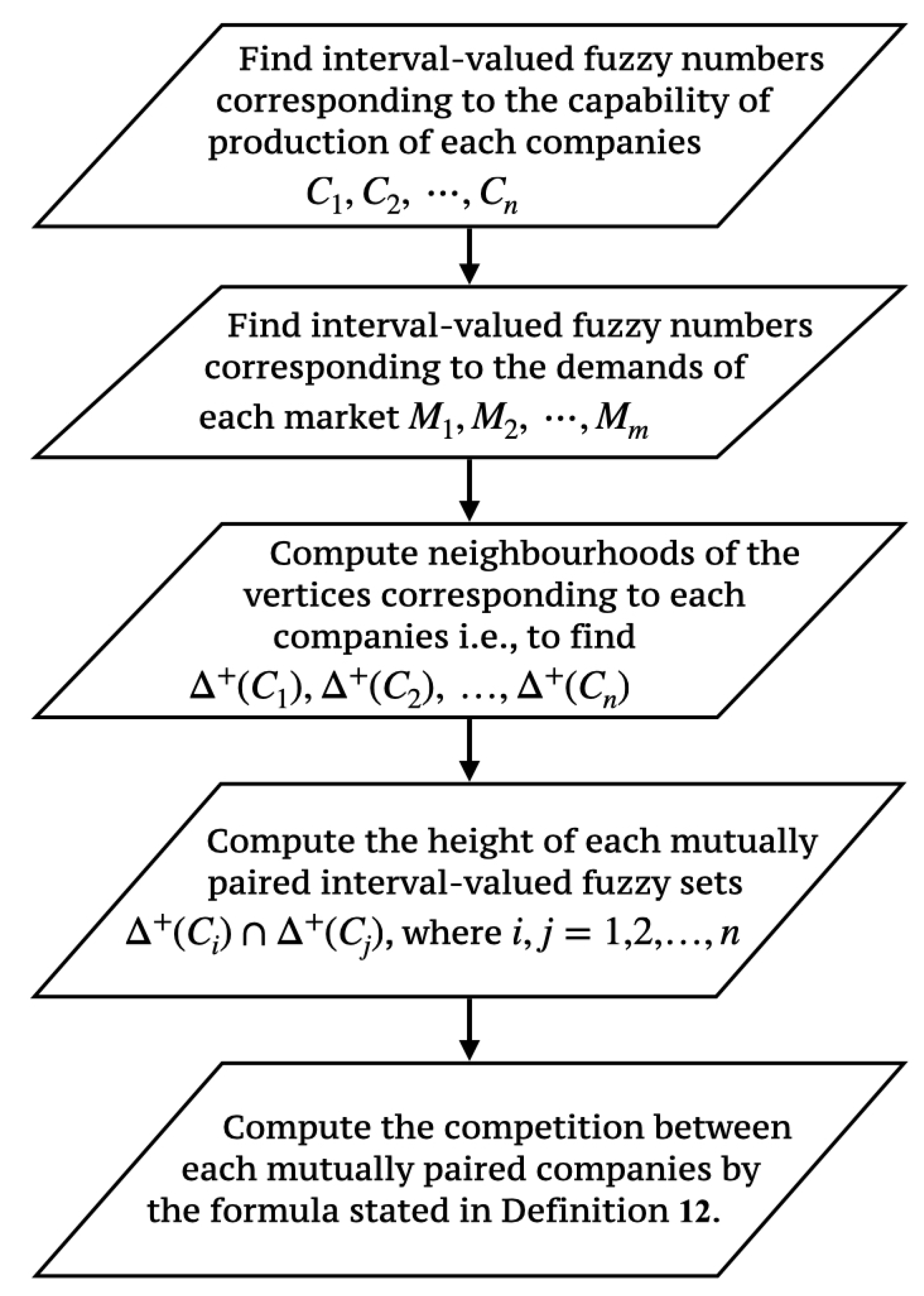
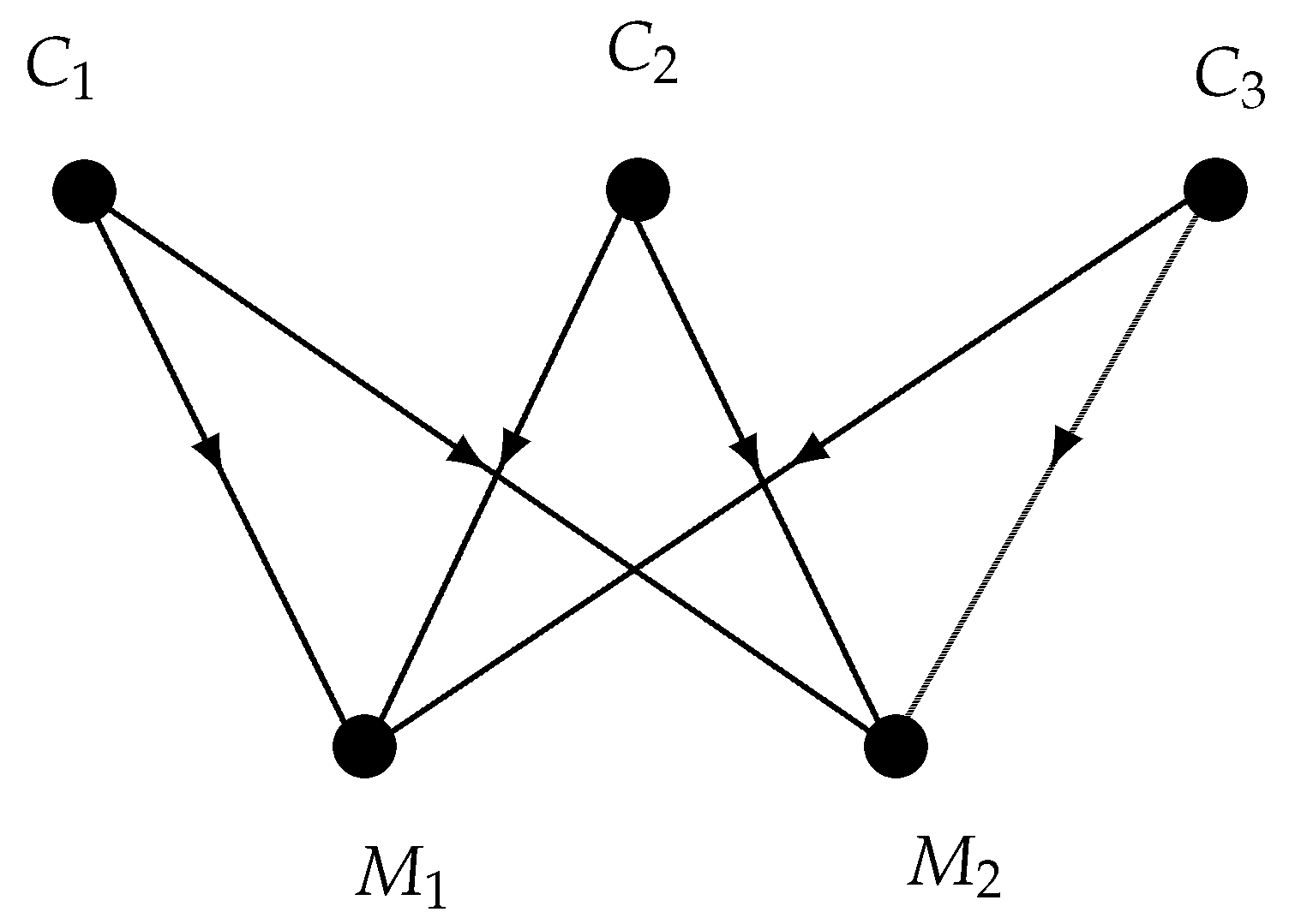
4. An Application of IVFCG in Manufacturing Industries

Every manufacturing industry has several production company and markets to sell the product. Any production company produces their products as per market demands. They are also liable to transport the products to the market so that the end user can use their product within a reasonable time. They wish to deliver with minimum cost as much as they can. Market has the time-bound factor to get the production from company within a reasonable cost. Market has various opportunities to choose the company as well as company can choose market for their sake. So, there is fair competition between companies. The problem is to find out which companies are in competition and the strengths of their competition to achieve markets that they serve, considering all the cases of production, demands and the time that they can spare. This problem can be modeled as an IVFCG by considering the following correspondences:
  • Companies and markets are treated as vertices.
  • The membership values of vertices that are taken as companies is a sub-interval of [ 0 , 1 ] . The significance of this interval number is that every company has a minimum and maximum capability to produce the product. We have assigned a grade to each power of capabilities within the min-max range. So, the interval becomes a fuzzy interval number.
  • Similarly, assigning grade for demands that the market has, each vertex associated to a fuzzy interval number.
  • The company and market are connected, that is, they have an edge if they both have the same time tenure to transport or take the product. A grade is assigned to each time within the tenure. This membership grade is also a fuzzy interval number.
Assuming the company and market have higher membership values than that of their shared time, i.e., membership value of each edge is less than the minimum of membership values of all the vertices, the problem is well-defined for an IVFCG model.
To find the strength of competitions among companies in manufacturing industries, the calculation flow is shown as a flowchart in the Figure 6. To explain the problem, in particular, let us consider the following example.
Three companies namely, C 1 , C 2 and C 3 produces certain product. Each company has a capability to produce 20–70%, 87–98% and 90–100% of demands respectively. Each of these shadowiness in capability of production can be corresponded to interval-valued fuzzy numbers as [ 0.2 , 0.7 ] , [ 0.87 , 0.98 ] and [ 0.9 , 1 ] respectively, in fuzzy sense. There are two markets M 1 and M 2 . They have also 90–100% and 85–95% demands in market respectively. Amount of demands are also shadowy. These can be corresponded to interval-valued fuzzy numbers as [ 0.9 , 1 ] and [ 0.85 , 0.95 ] respectively. Similarly, the interval-valued fuzzy numbers for transportation time corresponding to the edges ( C 1 , M 1 ) , ( C 1 , M 2 ) , ( C 2 , M 1 ) , ( C 2 , M 2 ) , ( C 3 , M 1 ) and ( C 3 , M 2 ) can be taken as [ 0.1 , 0.4 ] , [ 0.2 , 0.6 ] , [ 0.85 , 0.9 ] , [ 0.75 , 0.95 ] , [ 0.8 , 0.95 ] and [ 0.8 , 0.9 ] respectively. The relationship is shown in Figure 7. Note that this is an interval-valued fuzzy complete bipartite graphs.
Now,
Δ + ( C 1 ) = { M 1 [ 0.1 , 0.4 ] , M 2 [ 0.2 , 0.6 ] } Δ + ( C 2 ) = { M 1 [ 0.85 , 0.9 ] , M 2 [ 0.75 , 0.95 ] } Δ + ( C 3 ) = { M 1 [ 0.8 , 0.95 ] , [ 0.8 , 0.9 ] }
Then,
h ( Δ + ( C 1 ) Δ + ( C 2 ) ) = h ( { M 1 [ 0.1 , 0.4 ] , M 2 [ 0.2 , 0.6 ] } ) = [ 0.2 , 0.6 ] h ( Δ + ( C 1 ) Δ + ( C 3 ) ) = h ( { M 1 [ 0.1 , 0.4 ] , M 2 [ 0.2 , 0.6 ] } ) = [ 0.2 , 0.6 ] h ( Δ + ( C 2 ) Δ + ( C 3 ) ) = h ( { M 1 [ 0.8 , 0.9 ] , M 2 [ 0.75 , 0.9 ] } ) = [ 0.8 , 0.9 ]
Therefore,
θ T ( C 1 , C 2 ) = [ 0.2 × 0.2 , 0.7 × 0.6 ] = [ 0.04 , 0.42 ] θ T ( C 1 , C 3 ) = [ 0.2 × 0.2 , 0.7 × 0.6 ] = [ 0.04 , 0.42 ] θ T ( C 2 , C 3 ) = [ 0.87 × 0.8 , 0.98 × 0.9 ] = [ 0.696 , 0.882 ] [ 0.70 , 0.88 ]
The corresponding IVFCG of Figure 7 is shown in Figure 8. The membership value (degree) of competition among the companies is shown in Table 2.
A complete analysis of the result is shown in the Table 3.
The diagrammatic representation is shown in Figure 9.

5. Implications

In the case of any kind of competitive interconnected system, each competitor verifies the ability and capability of his opponent. The observations we present are useful in determining the capabilities and capabilities of all competitors present in such systems. The strength and intensity of competition between any two competitors can be determined within an interval. As a result, although the strength of competition is correct, it is within an interval, so the scope of application of the method is wide. Theoretically, it has been shown the cases when and where the strength of a competitor becomes higher.

6. Conclusions

There are many works have been done on fuzzy competition graphs and its extensions. After the work of FCG, we feel the importance of IVFCG as many real problems like time-bound network-based technology, neurology, ecology, market demand, etc. demands the uses of such type of modelling introduced in this paper. There is a great deal to handle with homomorphism and isomorphism of IVFCG products that have done by proving them in this paper. The proposed method of IVFCG is much more useful for the analysis of any network related to competition. This method is very useful for solving real-world problems. Here interval-valued fuzzy set is used instead of a general fuzzy set. One of the biggest problems in the world of this civilization is the constant competition of the manufacturing industries. Here, the competitive strength of the manufacturing industries determined and described the position of a company in the market. But, the problem of manufacturing industries is even bigger. There is a need to solve various problems starting from economic problems to business communication, business relations etc. However, many real problems can occur where a relationship is bipolar, for example, let’s say two companies produce two types of products in a market where there is no competition but great cooperation. For example, if one company produces petrol-powered cars and the other company produces petrol, there should be no competition between them. In all these cases the problem can be solved by using bipolar fuzzy set in the case of Competition graphs. There are also opportunities to solve various real problems using intuitionistic fuzzy sets.

Author Contributions

Conceptualization, M.P.; Methodology, T.P.; Validation, G.M. and A.M.A.; Writing—original draft, G.M.; Writing—review and editing, A.M.A. All authors have read and agreed to the published version of the manuscript.

Funding

This research received no external funding.

Acknowledgments

The authors are grateful to the Editor-in-Chief and Honorable reviewers of the journal “Mathematics” for their suggestions to improve the quality and presentation of the paper.

Conflicts of Interest

The authors declare no conflict of interest.

References

  1. Cohen, J.E. Interval Graphs and Food Webs: A Finding and a Problem; RAND Corporation: Santa Monica, CA, USA, 1968. [Google Scholar]
  2. Rosenfeld, A. Fuzzy Graphs; Academic Press: New York, NY, USA, 1975; pp. 77–95. [Google Scholar]
  3. Zadeh, L.A. Similarity relations and fuzzy orderings. Inf. Sci. 1971, 3, 177–200. [Google Scholar] [CrossRef]
  4. Kim, S.R.; McKee, T.A.; McMorris, F.; Roberts, F.S. p-Competition graphs. Linear Algebra Appl. 1995, 217, 167–178. [Google Scholar] [CrossRef] [Green Version]
  5. Brigham, R.C.; McMorris, F.R.; Vitray, R.P. Tolerance competition graphs. Linear Algebra Appl. 1995, 217, 41–52. [Google Scholar] [CrossRef] [Green Version]
  6. Cho, H.H.; Kim, S.R.; Nam, Y. The m-step competition graph of a digraph. Discret. Appl. Math. 2000, 105, 115–127. [Google Scholar] [CrossRef] [Green Version]
  7. Sonnatag, M.; Teichert, H.M. Competition hypergraphs. Discret. Appl. Math. 2004, 143, 324–329. [Google Scholar] [CrossRef] [Green Version]
  8. Samanta, S.; Pal, M. Fuzzy k-competition graphs and p-competition fuzzy graphs. Fuzzy Inf. Eng. 2013, 5, 191–204. [Google Scholar] [CrossRef]
  9. Pramanik, T.; Samanta, S.; Sarkar, B.; Pal, M. Fuzzy ϕ-tolerance competition graphs. Soft Comput. 2017, 21, 3723–3734. [Google Scholar] [CrossRef]
  10. Pramanik, T.; Samanta, S.; Pal, M.; Mondal, S.; Sarkar, B. Interval-valued fuzzy ϕ-tolerance competition graphs. SpringerPlus 2016, 5, 1981. [Google Scholar] [CrossRef] [Green Version]
  11. Bhutani, K.R.; Battou, A. On M-strong fuzzy graphs. Inf. Sci. 2003, 155, 103–109. [Google Scholar] [CrossRef]
  12. Bhutani, K.R.; Rosenfeld, A. Strong arcs in fuzzy graphs. Inf. Sci. 2003, 152, 319–322. [Google Scholar] [CrossRef]
  13. Craine, W.L. Characterization of fuzzy interval graphs. Fuzzy Sets Syst. 1994, 68, 181–193. [Google Scholar] [CrossRef]
  14. Ghosh, P.; Kundu, K.; Sarkar, D. Fuzzy graph representation of a fuzzy concept lattice. Fuzzy Sets Syst. 2010, 161, 1669–1675. [Google Scholar] [CrossRef]
  15. Isaak, G.; Kim, S.R.; McKee, T.A.; McMorris, F.R.; Roberts, F.S. 2-competition graphs. SIAM J. Disc. Math. 1992, 5, 524–538. [Google Scholar] [CrossRef] [Green Version]
  16. Nayeem, S.M.A.; Pal, M. Shortest path problem on a network with imprecise edge weight. Fuzzy Optim. Decis. Mak. 2005, 4, 293–312. [Google Scholar] [CrossRef]
  17. Cable, C.; Jones, K.F.; Lundgren, J.R.; Seager, S. Niche graphs. Discret. Appl. Math. 1989, 23, 231–241. [Google Scholar] [CrossRef] [Green Version]
  18. Samanta, S.; Pal, M. Fuzzy tolerance graphs. Int. J. Latest Trends Math. 2011, 1, 57–67. [Google Scholar]
  19. Samanta, S.; Pal, M.; Pal, A. New concepts of fuzzy planar graphs. Int. J. Adv. Res. Artif. Intell. 2014, 3, 52–59. [Google Scholar] [CrossRef]
  20. Samanta, S.; Pal, M. Fuzzy planar graph. IEEE Trans. Fuzzy Syst. 2015, 23, 1936–1942. [Google Scholar] [CrossRef]
  21. Pramanik, T.; Samanta, S.; Pal, M. Interval-valued fuzzy planar graphs. Int. J. Mach. Learn. Cybern. 2016, 7, 653–664. [Google Scholar] [CrossRef]
  22. Rashmanlou, H.; Pal, M. Some properties of highly irregular interval-valued fuzzy graphs. World Appl. Sci. J. 2013, 27, 1756–1773. [Google Scholar]
  23. Samanta, S.; Pal, M. Irregular bipolar fuzzy graphs. Int. J. Appl. Fuzzy Sets 2012, 2, 91–102. [Google Scholar]
  24. Samanta, S.; Pramanik, T.; Pal, M. Fuzzy colouring of fuzzy graphs. Afr. Mat. 2016, 27, 37–50. [Google Scholar] [CrossRef]
  25. Rashmanlou, H.; Samanta, S.; Pal, M.; Borzooei, R.A. A study on bipolar fuzzy graphs. J. Intell. Fuzzy Syst. 2015, 28, 571–580. [Google Scholar] [CrossRef]
  26. Rashmanlou, H.; Pal, M. Isometry on interval-valued fuzzy graphs. Int. J. Fuzzy Math. Arch. 2014, 3, 28–35. [Google Scholar]
  27. Rashmanlou, H.; Pal, M. Balanced interval-valued fuzzy graphs. J. Phys. Sci. 2013, 17, 43–57. [Google Scholar]
  28. Rashmanlou, H.; Pal, M. Antipodal interval-valued fuzzy graphs. Int. J. Appl. Fuzzy Sets Artif. Intell. 2013, 3, 107–130. [Google Scholar]
  29. Samanta, S.; Pal, M. Fuzzy threshold graphs. CiiT Int. J. Fuzzy Syst. 2011, 3, 1–9. [Google Scholar]
  30. Samanta, S.; Pal, M. Some more results on bipolar fuzzy sets and bipolar fuzzy intersection graphs. J. Fuzzy Math. 2014, 22, 253–262. [Google Scholar]
  31. Samanta, S.; Akram, M.; Pal, M. m-step fuzzy competition graphs. J. Appl. Math. Comput. 2015, 47, 461–472. [Google Scholar] [CrossRef]
  32. Voskoglou, M. Applications of Fuzzy Logic to Systems’ Modelling. Int. J. Fuzzy Syst. Appl. 2015, 3, 1–15. [Google Scholar] [CrossRef]
  33. Voskoglou, M. 3.7—A Stochastic Model for the Modelling Process. In Mathematical Modelling; Haines, C., Galbraith, P., Blum, W., Khan, S., Eds.; Woodhead Publishing: Cambridge, UK, 2007; pp. 149–157. [Google Scholar] [CrossRef]
  34. Voskoglou, M.G. A Fuzzy Model For Analogical Problem Solving. Int. J. Fuzzy Log. Syst. 2012, 2, 10–11. [Google Scholar] [CrossRef]
  35. Gil, R.A.; Johanyák, Z.C.; Kovács, T. Surrogate model based optimization of traffic lights cycles and green period ratios using microscopic simulation and fuzzy rule interpolation. Int. J. Artif. Intell. 2018, 16, 20–40. [Google Scholar]
  36. Hedrea, E.L.; Precup, R.E.; Bojan-Dragos, C.A. Results on Tensor Product-based Model Transformation of Magnetic Levitation Systems. Acta Polytech. Hung. 2019, 16. [Google Scholar]
  37. Deveci, M.; Öner, S.C.; Canıtez, F.; Öner, M. Evaluation of service quality in public bus transportation using interval-valued intuitionistic fuzzy QFD methodology. Res. Transp. Bus. Manag. 2019, 33, 100387. [Google Scholar] [CrossRef]
  38. Deveci, M.; Cali, U.; Kucuksari, S.; Erdogan, N. Interval type-2 fuzzy sets based multi-criteria decision-making model for offshore wind farm development in Ireland. Energy 2020, 117317. [Google Scholar] [CrossRef]
  39. Deveci, M.; Demirel, N.C. A survey of the literature on airline crew scheduling. Eng. Appl. Artif. Intell. 2018, 74, 54–69. [Google Scholar] [CrossRef]
  40. Canitez, F.; Deveci, M. An integration model for car sharing and public transport: Case of Istanbul. In Proceedings of the Accessible sur ResearchGate, Istanbul, Turkey, 2–3 November 2017. [Google Scholar]
  41. Deveci, M.; Demirel, N.Ç.; John, R.; Özcan, E. Fuzzy multi-criteria decision making for carbon dioxide geological storage in Turkey. J. Nat. Gas Sci. Eng. 2015, 27, 692–705. [Google Scholar] [CrossRef] [Green Version]
  42. Mordeson, J.N.; Nair, P.S. Cycles and cocycles of fuzzy graphs. Inf. Sci. 1996, 90, 39–49. [Google Scholar] [CrossRef]
  43. Samanta, S.; Pal, M.; Pal, A. Some more results on fuzzy k-competition graphs. Int. J. Adv. Res. Artif. Intell. 2014, 3, 60–67. [Google Scholar] [CrossRef]
  44. Akram, M.; Dudek, W.A. Interval-valued fuzzy graphs. Comput. Math. Appl. 2011, 61, 289–299. [Google Scholar] [CrossRef] [Green Version]
  45. Mordeson, J.N.; Nair, P.S. Fuzzy Graphs and Hypergraphs, 1st ed.; Physica: Heidelberg, Germany, 2000. [Google Scholar] [CrossRef]
  46. Eslahchi, C.; Onaghe, B.N. Vertex strength of fuzzy graphs. Int. J. Math. Math. Sci. 2006, 2006, 1–9. [Google Scholar] [CrossRef]
  47. Nagoorgani, A.; Hussain, R.J. Fuzzy effective distance k-dominating sets and their applications. Int. J. Algorith. Comput. Math. 2009, 2, 25–36. [Google Scholar]
  48. Nagoorgani, A.; Radha, K. On regular fuzzy graphs. J. Phys. Sci. 2008, 12, 33–40. [Google Scholar]
  49. Nagoorgani, A.; Latha, A. On irregular fuzzy graphs. Appl. Math. Sci. 2012, 6, 517–523. [Google Scholar]
  50. Mordeson, J.N.; Nair, P.S. Successor and source of (fuzzy) finite state machines and (fuzzy) directed graphs. Inf. Sci. 1996, 95, 113–124. [Google Scholar] [CrossRef]
  51. Goetschel, R.H. Introduction to fuzzy hypergraphs and Hebbian structures. Fuzzy Sets Syst. 1995, 76, 113–130. [Google Scholar] [CrossRef]
  52. McAllister, M.L.N. Fuzzy intersection graphs. Comput. Math. Appl. 1988, 15, 871–886. [Google Scholar] [CrossRef] [Green Version]
  53. Zhang, W.R. Bipolar fuzzy sets and relations: A computational framework for cognitive modeling and multiagent decision analysis. Proc. IEEE Conf. 1994, 309, 305–309. [Google Scholar]
  54. Akram, M. Bipolar fuzzy graphs with applications. Knowl. Based Syst. 2013, 39, 1–8. [Google Scholar] [CrossRef]
  55. Akram, M. Interval-valued fuzzy line graphs. Neural Comput. Appl. 2012, 21, 145–150. [Google Scholar] [CrossRef]
Figure 1. An example of a food web.
Mathematics 08 01008 g001
Figure 2. An IVFDG.
Figure 2. An IVFDG.
Mathematics 08 01008 g002
Figure 3. IVFCG of the IVFDG shown in Figure 2.
Mathematics 08 01008 g003
Figure 4. An example that an IVFCG have no independent strong edge although all the edges are independent strong in IVFDG.
Mathematics 08 01008 g004
Figure 5. An example of interval-valued fuzzy 2-step CG.
Mathematics 08 01008 g005
Figure 6. Flowchart of the work flow to compute the strength of competitions among companies in manufacturing industries.
Mathematics 08 01008 g006
Figure 7. The relationship between companies and markets.
Mathematics 08 01008 g007
Figure 8. IVFCG of Figure 7.
Mathematics 08 01008 g008
Figure 9. Competition among three companies.
Mathematics 08 01008 g009
Table 1. Comparison of the work to the existing research work.
AuthorYearContributionsRemarks
Cohen [1]1968Use of interval graphs in food websDeals only with crisp graph
Kim et al. [4]1995p-Competition graph of a digraphFurther variation of crisp competition graph
Brigham et al. [5]1995Tolerance competition graphDeals with the competition graphs where tolerances matter
Cho et al. [6]2000m-Step competition graph of a digraphAnother variation of a competition graph
Sonnatag and Teichert [7]2004Competition hypergraphsCompetition is studied in hypergraphs
Samanta and Pal [8]2013Fuzzy k-Competition graphs and p-Competition graphsFuzziness is considered in the earlier two types of crisp graphs
Pramanik et al. [9]2017Fuzzy ϕ -tolerance competition graphsFuzziness is considered in more general version of tolerance competition graphs
Pramanik et al. [10]2016Interval-valued fuzzy ϕ -tolerance competition graphsMore general fuzzy system is considered in fuzzy ϕ -tolerance competition graphs
Pramanik et al. (This paper)____In this paper, fuzzy values of all the network problems related to competition are also taken as intervals. As a result much more generalizations have been madeMore generalized concept than all previous existing research works.
Table 2. Degree of Competition among the Companies.
CompaniesDegree of CompetitionCompetition in %
C 1 , C 2 [ 0.04 , 0.42 ] [ 4 , 42 ]
C 2 , C 3 [ 0.70 , 0.88 ] [ 70 , 88 ]
C 3 , C 1 [ 0.04 , 0.42 ] [ 4 , 42 ]
Table 3. Analysis of the result obtained in the problem of manufacturing industries.
Description of the ResultResult ObtainedAnalysis of the Result
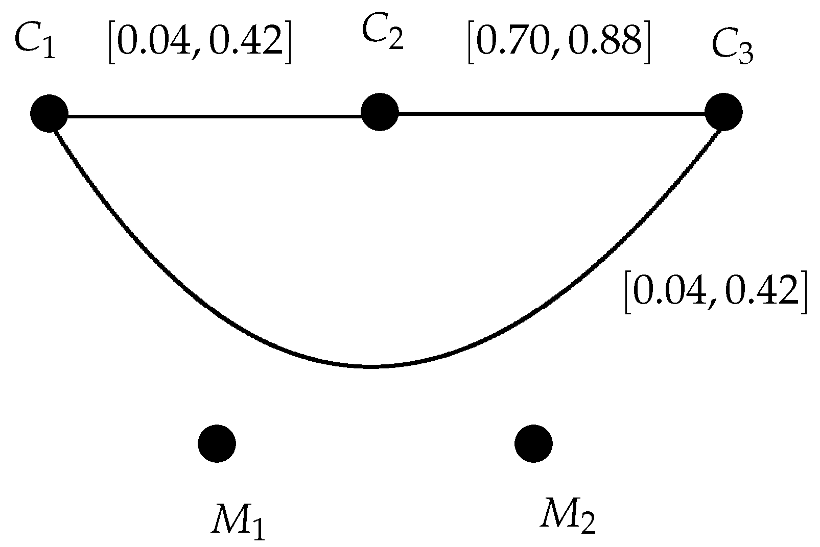
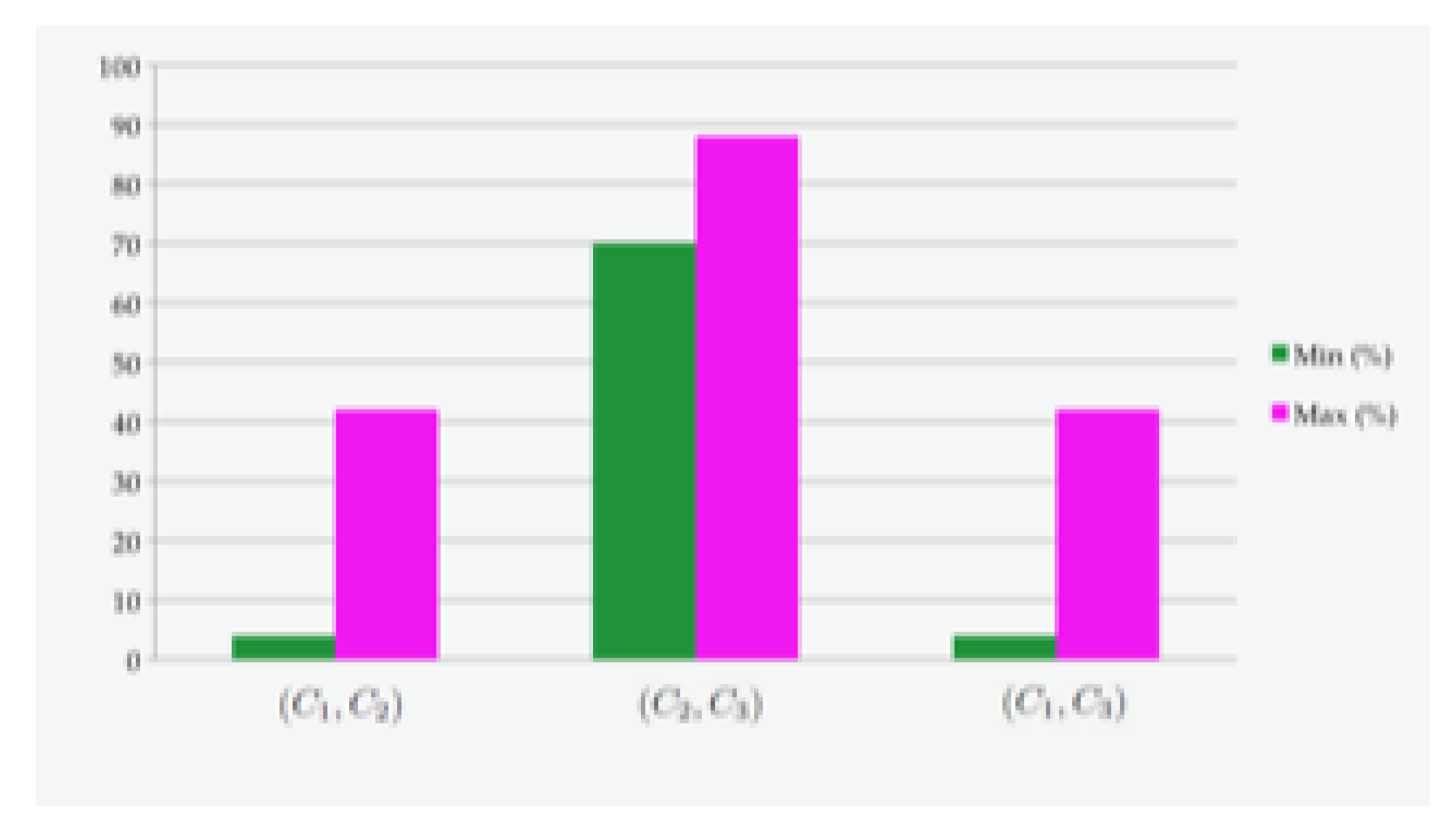
Highest degree of competition among companies [ 0.70 , 0.88 ] This result shows that the companies have at least 70% and at most 88% competitions in the market (Computations made using the formula stated in Definition 1)
Independent strength of competition between the companies C 2 and C 3 0.70 min { 0.87 , 0.9 } , 0.88 min { 0.98 , 1 } = [ 0.80 , 0.90 ] > [ 0.5 , 0.5 ] The height of interval-valued fuzzy set Δ + ( C 2 ) Δ + ( C 3 ) is [0.8, 0.9] which is greater than [ 0.5 , 0.5 ] . So there is a strong competition between the two companies C 2 and C 3 (Refer Theorem 2)

