A New Machine Learning Algorithm Based on Optimization Method for Regression and Classification Problems

Abstract

A convex minimization problem in the form of the sum of two proper lower-semicontinuous convex functions has received much attention from the community of optimization due to its broad applications to many disciplines, such as machine learning, regression and classification problems, image and signal processing, compressed sensing and optimal control. Many methods have been proposed to solve such problems but most of them take advantage of Lipschitz continuous assumption on the derivative of one function from the sum of them. In this work, we introduce a new accelerated algorithm for solving the mentioned convex minimization problem by using a linesearch technique together with a viscosity inertial forward–backward algorithm (VIFBA). A strong convergence result of the proposed method is obtained under some control conditions. As applications, we apply our proposed method to solve regression and classification problems by using an extreme learning machine model. Moreover, we show that our proposed algorithm has more efficiency and better convergence behavior than some algorithms mentioned in the literature.

1. Introduction

In this work, we are dealing with a convex minimization problem, which can be formulated as

$$\underset{x\in H}{min}\{f\left(x\right)+g\left(x\right)\},$$

(1)

where $f,g:H\to \mathbb{R}\cup \{+\infty \}$ are proper, lower-semicontinuous convex functions and H is a Hilbert space. Many real world problems, such as signal processing, image reconstruction and compressed sensing, can be described using this model [1,2,3,4]. Moreover, data classification can also be formulated as (1); for more information about the importance and development of data classification and its methods see [5,6,7,8]. Therefore, a convex minimization problem has a wide range of applications, some of which will be studied in this research.

If f is differentiable then it is well-known that an element $x\in H$ is a solution of (1) if and only if

$$x=pro{x}_{\alpha g}(I-\alpha ▿f)\left(x\right),$$

(2)

where $\alpha >0,$ $pro{x}_{\alpha g}\left(x\right)=J_{\alpha }^{\partial g}\left(x\right)={(I-\alpha \partial g)}^{-1}\left(x\right),$ I is an identity mapping, and $\partial g$ is a subdifferential of $g.$ In addition, if $▿f$ is L-Lipschitz continuous then the classical foward–backward algorithm [9] can be used to solve (1). It is defined as follows:

$$x_{n+1}=pro{x}_{{\alpha }_{n}g}(I-{\alpha }_n▿f)\left(x_n\right)$$

(3)

where ${\alpha }_n$ is a suitable stepsize. This method has been extensively used due to its simplicity, as a result it has been improved by many works, as seen in [2,10,11,12]. One well-known method that has improved the convergence rate of (3) significantly is known as the fast iterative shrinkage-threshodling algorithm or FISTA. It was proposed by Beck and Teboulle [13], as seen in Algorithm 1.

Algorithm 1. FISTA.

1: Input $x_1=y_0\in H,t_1=1,L>0,k=\mathrm{number\; of\; iterations}.$

2: for $n=1$ to k do

3:     $y_n=pro{x}_{\frac{1}{L}g}(x_n-\frac{1}{L}▿f{x}_n),$

4:     $t_{n+1}=\frac{1+\sqrt{1+4t_n^2}}{2},$

5:     ${\theta }_n=\frac{t_n-1}{t_{n+1}},$

6:     $x_{n+1}=y_n+{\theta }_n(y_n-y_{n-1}).$

7: end for

8: return $x_{n+1}$

They proved that FISTA has a better convergence rate than (3), however the convergence theorem of this method was not given. Recently, Laing and Schonlieb [14] modified FISTA by setting $t_{n+1}=\frac{p+\sqrt{q+r{t}_n^2}}{2},$ where $p,q>0$ and $0<r\le 4,$ and proved its weak convergence theorem.

In the case that H is an infinite dimension Hilbert space, weak convergence results may not be enough, consequently modifications of some algorithms are needed to obtain strong convergence results. There are several ways to modify the methods for such purpose, for more information see [15,16,17,18]. One method that caught our attention was the viscosity-base inertial foward–backward algorithm (VIFBA) proposed by Verma et al. [19], as seen in Algorithm 2.

Algorithm 2. VIFBA.

1: Input $x_0,x_1\in H,L>0,{\beta }_n\ge 0,{\alpha }_n\in (0,1),{\gamma }_n\in (0,\frac{2}{L}),c$-contractive mapping F,       $k=\mathrm{number\; of\; iterations}.$

2: for $n=1$ to k do

3:     $y_n=x_n+{\beta }_n(x_n-x_{n-1}),$

4:     $z_n={\alpha }_{n}F\left(y_n\right)+(1-{\alpha }_n)y_n$,

5:     $x_{n+1}=pro{x}_{{\gamma }_{n}g}(z_n-{\gamma }_n▿f{z}_n)$.

6: end for

7: return $x_{n+1}$

They proved a strong convergence of this algorithm if the following conditions are satisfied for all $n\in \mathbb{N}$:

A1.

${\displaystyle \underset{n\to \infty }{lim}{\alpha }_n=0,}$ and ${\displaystyle \sum _{n=1}^{\infty }{\alpha }_n=\infty ,}$

A2.

${\gamma }_n\in (0,\frac{2}{L}),$ and ${\displaystyle \sum _{n=1}^{\infty }|{\gamma }_n-{\gamma }_{n+1}|<\infty ,}$

A3.

${\displaystyle \sum _{n=1}^{\infty }{\Vert x_{n+1}-x_n\Vert }^2<\infty ,}$ and ${\displaystyle \underset{n\to \infty }{lim}\frac{{\beta }_n\Vert x_n-x_{n-1}\Vert }{{\alpha }_n}=0.}$

Note that all the methods mentioned above require $▿f$ to be L-Lipschitz continuous, which is quite difficult to find in general. Therefore, some improvements are still desirable.

Very recently, Cruz and Nghia [20] proposed a linesearch technique which can be used to eliminate the L-Lipschitz continuous assumption of $▿f$ and replaced it with weaker assumptions. In their work, the following conditions are needed instead:

B1.

$f,g$ are proper lower semicontinuous convex functions with $domg=domf,$

B2.

f is differentiable on an open set containing $domg,$ and $▿f$ is uniformly continuous on any bounded subset of $domg$ and maps any a bounded subset of $domg$ to a bounded set in $H.$

The linesearch step is defined as Algorithm 3 as follows.

Algorithm 3. Linesearch 1.

1: Input $x\in domg,$ $\sigma >0$, $\theta \in (0,1),$ and $\delta \in (0,\frac{1}{2}).$

2: set $\alpha =\sigma .$

3: while $\alpha \Vert ▿f\left(pro{x}_{\alpha g}(x-\alpha ▿fx)\right)-▿fx\Vert >\delta \Vert pro{x}_{\alpha g}(x-\alpha ▿fx)-x\Vert$ do

4:   $\alpha =\theta \alpha .$

5: end while

6: return $\alpha$

They also proved that Linesearch 1 stops after finitely many steps, and proposed Algorithm 4 as follows.

Algorithm 4.

1: Input $x_1\in domg,$ $\sigma >0$, $\theta \in (0,1),$ and $\delta \in (0,\frac{1}{2}),k=\mathrm{number\; of\; iterations}.$

2: for $n=1$ to k do

3:     ${\gamma }_n=$ Linesearch 1$(x_n,\sigma ,\theta ,\delta ),$

4:     $x_{n+1}=pro{x}_{{\gamma }_{n}g}(I-{\gamma }_n▿f)\left(x_n\right).$

5: end for

6: return $x_{n+1}$

They also proved its weak convergence theorem. Again the weak convergence may not be enough in the context of infinite dimension space.

As we know, most of the work related to a convex minimization problem assumes the L-Lipschitz continuity of $▿f$. This restriction can be relaxed using a linesearch technique. So, we are motivated to establish a novel accelerated algorithm for solving a convex minimization problem (1), which employs a linesearch technique introduced by Cruz and Nghia [20] together with VIFBA [19]. The novelty of our proposed method is a suitable combination of the two methods to obtain a fast and efficient method for solving (1). We improve Algorithm 4 by adding an inertial step, which enhances the performance of the algorithm. We also prove its strong convergence theorem under weaker assumptions on the control conditions than that of VIFBA. More precisely, we can eliminate the assumption A2 and replace A3 with a weaker assumption. As applications, we apply our main result to solve a data classification problem and a regression of a sine function. Then we compare the performance of our algorithm with FISTA, VIFBA, and Algorithm 4.

This work is organized as follows: In Section 2, we recall some useful concepts related to the topic. In Section 3, we provide a new algorithm and prove its strong convergence to a solution of (1). In Section 4, we conduct some numerical experiments with a data classification problem and a regression of a sine function and compare the performance of each algorithm (FISTA, VIFBA, Algorithms 4 and 5). Finally, the conclusion of this work is in Section 5.

2. Preliminaries

In this section, we review some important tools which will be used in the later sections. Throughout this paper, we denote $x_n\to x$ and $x_n\rightharpoonup x$ as strong and weak convergence of $\left\{x_n\right\}$ to $x,$ respectively.

A mapping $T:H\to H$ is said to be L-Lipschitz continuous if there exists $L>0$ such that

$$\Vert Tx-Tx\Vert \le L\Vert x-y\Vert ,\mathrm{for}\mathrm{all}x,y\in H.$$

For $x\in H,$ a subdifferential of h at x is defined as follows:

$$\partial h\left(x\right):=\{u\in H:⟨u,y-x⟩+h(x)\le h(y),y\in H\}.$$

We have known from [21] that a subdifferential $\partial h$ is maximal monotone. Moreover, a graph of $\partial h,$ $Gph(\partial h):=\left\{\right(u,v)\in H\times H:v\in \partial h(u\left)\right\}$ is demiclosed, i.e., for any sequence $(u_n,v_n)\in Gph(\partial h)$ such that $\left\{u_n\right\}$ converges weakly to u and $\left\{v_n\right\}$ converges strongly to $v,$ we have $(u,v)\in Gph(\partial h)$.

The proximal operator, $pro{x}_g:H\to domg$ with $pro{x}_g\left(x\right)={(I+\partial g)}^{-1}\left(x\right)$, is single-valued with a full domain. Moreover, the following is satisfied:

$$\frac{x-pro{x}_{\alpha g}x}{\alpha }\in \partial g\left(pro{x}_{\alpha g}x\right),\mathrm{for} \mathrm{all}x\in H \mathrm{and} \alpha >0.$$

(4)

The following lemmas are crucial for the main results.

Lemma 1

([22]). Let $f,g:H\to \mathbb{R}$ be two proper lower semicontinuous convex functions with $domg\subseteq domf$ and $J(x,\alpha )=pro{x}_{\alpha g}(x-\alpha ▿fx).$ Then for any $x\in domg$ and ${\alpha }_2\ge {\alpha }_1>0,$ we have

$$\frac{{\alpha }_2}{{\alpha }_1}\Vert x-J(x,{\alpha }_1)\Vert \ge \Vert x-J(x,{\alpha }_2)\Vert \ge \Vert x-J(x,{\alpha }_1)\Vert .$$

Lemma 2

([23]). Let H be a real Hilbert space. Then the following holds, for all $x,y\in H$ and $\alpha \in [0,1]$,

(i) 

${\Vert x\pm y\Vert }^2={\Vert x\Vert }^2\pm 2⟨x,y⟩+{\Vert y\Vert }^2,$

(ii) 

${\Vert \alpha x+(1-\alpha )y\Vert }^2={\alpha \Vert x\Vert }^2+{(1-\alpha )\Vert y\Vert }^2-\alpha (1-\alpha ){\Vert x-y\Vert }^2,$

(iii) 

${\Vert x+y\Vert }^2\le {\Vert x\Vert }^2+2⟨y,x+y⟩.$

Lemma 3

([24]). Let $\left\{a_n\right\}$ be a sequence of real numbers such that there exists a subsequence $\left\{a_{m_j}\right\}$ of $\left\{a_n\right\}$ such that $a_{m_j}<a_{m_j+1}$ for all $j\in \mathbb{N}.$ Then there exists a nondecreasing sequence $\left\{n_k\right\}$ of $\mathbb{N}$ such that ${\displaystyle \underset{k\to \infty }{lim}{n}_k=\infty }$ and for all sufficiently large $k\in \mathbb{N}$ the following holds:

$$a_{n_k}\le a_{n_k+1}and{a}_k\le a_{n_k+1}.$$

Lemma 4

([25]). Let $\left\{a_n\right\}$ be a sequence of nonnegative real numbers, $\left\{{\alpha }_n\right\}$ a sequence in $(0,1)$ with ${\displaystyle \sum _{n=1}^{\infty }{\alpha }_n=\infty }$, $\left\{b_n\right\}$ a sequence of nonnegative real numbers with ${\displaystyle \sum _{n=1}^{\infty }{b}_n<\infty }$ and $\left\{{\zeta }_n\right\}$ a sequence of real numbers with ${\displaystyle \underset{n\to \infty }{lim\; sup}{\zeta }_n\le 0.}$ Suppose that the following holds

$$a_{n+1}\le (1-{\alpha }_n)a_n+{\alpha }_n{\zeta }_n+b_n,$$

for all $n\in \mathbb{N}$, then ${\displaystyle \underset{n\to \infty }{lim}{a}_n=0.}$

3. Main Results

In this section, we assume the existence of a solution of (1) and denote $S_{*}$ the set of all such solutions. It is known that $S_{*}$ is closed and convex. We propose a new algorithm, by combining a linesearch technique (Linesearch 1) with VIFBA, as seen in Algorithm 5. A diagram of this algorithm can be seen in Figure 1.

Algorithm 5:

1: Input $x_0,x_1\in H,\sigma >0,\theta \in (0,1),\delta \in (0,\frac{1}{2}),{\beta }_n\ge 0,{\alpha }_n\in (0,1),c$-contractive mapping      $F,k=$ number of iterations.

2: for $n=1$ to k do

3:     $y_n=x_n+{\beta }_n(x_n-x_{n-1}),$

4:     $z_n={\alpha }_{n}F\left(y_n\right)+(1-{\alpha }_n)y_n$,

5:     ${\gamma }_n=$ Linesearch 1$(z_n,\sigma ,\theta ,\delta )$,

6:     $x_{n+1}=pro{x}_{{\gamma }_{n}g}(z_n-{\gamma }_n▿f{z}_n)$.

7: end for

8: return $x_{n+1}$

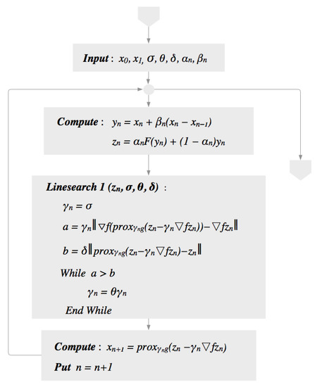
Figure 1. Diagram of Algorithm 5.

We prove a strong convergence result of Algorithm 5 in Theorem 1 as follows.

Theorem 1.

Let H be a Hilbert space, $g:H\to \mathbb{R}\cup \{+\infty \}$ proper lower-semicontinuous convex, $f:H\to \mathbb{R}\cup \{+\infty \}$ proper convex differentiable with $▿f$ being uniformly continuous on any bounded subset of $H.$ Suppose the following holds:

C1. 

${\displaystyle \underset{n\to \infty }{lim}{\alpha }_n=0,\sum _{n=1}^{\infty }{\alpha }_n=\infty ,}$

C2. 

${\displaystyle \underset{n\to \infty }{lim}\frac{{\beta }_n}{{\alpha }_n}\Vert x_n-x_{n-1}\Vert =0.}$

Then a sequence $\left\{x_n\right\}$ generated by Algorithm 5 converges strongly to $x^{*}=P_{S_{*}}F\left(x^{*}\right).$

Proof. 

Since $S_{*}$ is closed and convex, a mapping $P_{S_{*}}F$ yields a fixed point. Let $x^{*}=P_{S_{*}}F\left(x^{*}\right),$ by the definition of $x_n,y_n$ and $z_n$, we obtain the following, for all $n\in \mathbb{N}$:

$$\Vert x_n-y_n\Vert ={\beta }_n\Vert x_n-x_{n-1}\Vert =\frac{{\beta }_n}{{\alpha }_n}\Vert x_n-x_{n-1}\Vert {\alpha }_n\to 0\mathrm{as}n\to \infty ,$$

(5)

$$\Vert z_n-y_n\Vert ={\alpha }_n\Vert F{y}_n-y_n\Vert ,\mathrm{and}$$

(6)

$$\Vert y_n-x^{*}\Vert \le \Vert x_n-x^{*}\Vert +\frac{{\beta }_n}{{\alpha }_n}\Vert x_n-x_{n-1}\Vert {\alpha }_n\le \Vert x_n-x^{*}\Vert +{\alpha }_n{M}_1$$

(7)

for some $M_1\ge \frac{{\beta }_n}{{\alpha }_n}\Vert x_n-x_{n-1}\Vert .$ The following also holds:

$$\begin{array}{cc}\hfill \Vert y_n-x^{*}{\Vert }^2& \le \Vert x_n-x^{*}{\Vert }^2+2{\beta }_n\Vert x_n-x^{*}\Vert \Vert x_n-x_{n-1}\Vert +{\beta }_n{\Vert x_n-x_{n-1}\Vert }^2\hfill \\ \hfill & =\Vert x_n-x^{*}{\Vert }^2+\frac{{\beta }_n}{{\alpha }_n}\Vert x_n-x_{n-1}\Vert (2{\alpha }_n\Vert x_n-x^{*}\Vert +{\alpha }_n{\beta }_n\Vert x_n-x_{n-1}\Vert ),\forall n\in \mathbb{N}.\hfill \end{array}$$

(8)

Next, we prove the following

$$\Vert z_n-x^{*}{\Vert }^2-\Vert x_{n+1}-x^{*}{\Vert }^2\ge (1-2\delta ){\Vert x_{n+1}-z_n\Vert }^2.$$

(9)

Indeed, from (4) and the definition of $\partial g,$ we obtain

$$\frac{z_n-x_{n+1}}{{\gamma }_n}-▿f{z}_n\in \partial g\left(x_{n+1}\right), \mathrm{therefore}$$

$$g{x}^{*}-g{x}_{n+1}\ge ⟨\frac{z_n-x_{n+1}}{{\gamma }_n}-▿f{z}_n,x^{*}-x_{n+1}⟩, \mathrm{also}$$

$$f{x}^{*}-f{z}_n\ge ⟨▿f{z}_n,x^{*}-z_n⟩, \mathrm{and}$$

$$f{z}_n-f{x}_{n+1}\ge ⟨▿f{x}_{n+1},z_n-x_{n+1}⟩.$$

Hence, by using the above inequalities and the definition of ${\gamma }_n$, we have

$$\begin{array}{cc}\hfill f{x}^{*}-f{z}_n+g{x}^{*}-g{x}_{n+1}& \ge \frac{1}{{\gamma }_n}⟨z_n-x_{n+1},x^{*}-x_{n+1}⟩+⟨▿f{z}_n,x_{n+1}-z_n⟩,\hfill \\ \hfill & =\frac{1}{{\gamma }_n}⟨z_n-x_{n+1},x^{*}-x_{n+1}⟩+⟨▿f{z}_n-▿f{x}_{n+1},x_{n+1}-z_n⟩\hfill \\ \hfill & +⟨▿f{x}_{n+1},x_{n+1}-z_n⟩,\hfill \\ \hfill & \ge \frac{1}{{\gamma }_n}⟨z_n-x_{n+1},x^{*}-x_{n+1}⟩-\Vert ▿f{z}_n-▿f{x}_{n+1}\Vert \Vert x_{n+1}-z_n\Vert \hfill \\ \hfill & +⟨▿f{x}_{n+1},x_{n+1}-z_n⟩,\hfill \\ \hfill & \ge \frac{1}{{\gamma }_n}⟨z_n-x_{n+1},x^{*}-x_{n+1}⟩-\frac{\delta }{{\gamma }_n}{\Vert x_{n+1}-z_n\Vert }^2+f{x}_{n+1}-f{z}_n.\hfill \end{array}$$

Consequently,

$$\frac{1}{{\gamma }_n}⟨z_n-x_{n+1},x_{n+1}-x^{*}⟩\ge (f+g)\left(x_{n+1}\right)-(f+g)\left(x^{*}\right)-\frac{\delta }{{\gamma }_n}{\Vert x_{n+1}-z_n\Vert }^2.$$

Since $⟨z_n-x_{n+1},x_{n+1}-x^{*}⟩=\frac{1}{2}(\Vert z_n-x^{*}{\Vert }^2-\Vert z_n-x_{n+1}{\Vert }^2-\Vert x_{n+1}-x^{*}{\Vert }^2),$

$$\frac{1}{2{\gamma }_n}(\Vert z_n-x^{*}{\Vert }^2-\Vert z_n-x_{n+1}{\Vert }^2-\Vert x_{n+1}-x^{*}{\Vert }^2)\ge (f+g)\left(x_{n+1}\right)-(f+g)\left(x^{*}\right)-\frac{\delta }{{\gamma }_n}{\Vert x_{n+1}-z_n\Vert }^2.$$

Furthermore, it follows from $x^{*}\in S_{*}$ that

$$\begin{array}{cc}\hfill \Vert z_n-x^{*}{\Vert }^2-{\Vert x_{n+1}-x^{*}\Vert }^2& \ge 2{\gamma }_n[(f+g)\left(x_{n+1}\right)-(f+g)\left(x^{*}\right)]+(1-2\delta ){\Vert x_{n+1}-z_n\Vert }^2,\hfill \\ \hfill & \ge (1-2\delta )\Vert x_{n+1}-z_n{\Vert }^2.\hfill \end{array}$$

Next, we show that $\left\{x_n\right\}$ is bounded. Indeed, from (7) and (9), we obtain

$$\begin{array}{cc}\hfill \Vert x_{n+1}-x^{*}\Vert \le \Vert z_n-x^{*}\Vert & =\Vert {\alpha }_{n}F{y}_n+(1-{\alpha }_n)y_n-x^{*}\Vert ,\hfill \\ \hfill & \le {\alpha }_n\Vert F{y}_n-F{x}^{*}\Vert +{\alpha }_n\Vert F{x}^{*}-x^{*}\Vert +(1-{\alpha }_n)\Vert y_n-x^{*}\Vert ,\hfill \\ \hfill & \le (1-(1-c){\alpha }_n)\Vert y_n-x^{*}\Vert +{\alpha }_n\Vert F{x}^{*}-x^{*}\Vert ,\hfill \\ \hfill & \le (1-(1-c){\alpha }_n)\Vert x_n-x^{*}\Vert +(1-(1-c){\alpha }_n){\alpha }_n{M}_1+{\alpha }_n\Vert F{x}^{*}-x^{*}\Vert ,\hfill \\ \hfill & \le (1-(1-c){\alpha }_n)\Vert x_n-x^{*}\Vert +{\alpha }_n(1-c)\left(\frac{M_1+\Vert F{x}^{*}-x^{*}\Vert }{1-c}\right).\hfill \end{array}$$

Inductively, we have ${\displaystyle \Vert x_{n+1}-x^{*}\Vert \le max\{\Vert x_0-x^{*}\Vert ,\frac{M_1+\Vert F{x}^{*}-x^{*}\Vert }{1-c}\},}$ and hence $\left\{x_n\right\}$ is bounded. Furthermore, by using (5) and (6), $\left\{y_n\right\}$ and $\left\{z_n\right\}$ are also bounded. To show the convergence of $\left\{x_n\right\},$ we divide the proof into two cases.

Case 1 There exists $N_0\in \mathbb{N}$ such that $\Vert x_{n+1}-x^{*}\Vert \le \Vert x_n-x^{*}\Vert$ for all $n\ge N_0$. So ${\displaystyle \underset{n\to \infty }{lim}\Vert x_n-x^{*}\Vert =a,}$ for some $a\in \mathbb{R}.$ From (5) and (6), and the fact that

$$\Vert z_n-x^{*}\Vert \le \Vert z_n-y_n\Vert +\Vert y_n-x_n\Vert +\Vert x_n-x^{*}\Vert ,$$

we have ${\displaystyle \underset{n\to \infty }{lim}\Vert z_n-x^{*}\Vert =a.}$ Using (9), we have ${\displaystyle \underset{n\to \infty }{lim}\Vert x_{n+1}-z_n\Vert =0.}$ Since $\left\{z_n\right\}$ is bounded, there exists a subsequence $\left\{z_{n_k}\right\}$ of $\left\{z_n\right\}$ such that $z_{n_k}\rightharpoonup w,$ for some $w\in H,$ and the following holds:

$${\displaystyle \underset{n\to \infty }{lim\; sup}⟨F{x}^{*}-x^{*},z_n-x^{*}⟩=\underset{k\to \infty }{lim}⟨F{x}^{*}-x^{*},z_{n_k}-x^{*}⟩=⟨F{x}^{*}-x^{*},w-x^{*}⟩.}$$

We claim that $w\in S_{*}.$ In order to prove this, we need to consider two cases of $\left\{z_{n_k}\right\}.$ The first case, if ${\gamma }_{n_k}\ne \sigma ,$ for finitely many $k.$ Then, without loss of generality, we can assume that ${\gamma }_{n_k}=\sigma ,$ for all $k\in \mathbb{N}$. From the definition of ${\gamma }_{n_k},$ we have

$$\Vert ▿f{x}_{n_k+1}-▿f{z}_{n_k}\Vert \le \frac{\delta }{\sigma }\Vert x_{n_k+1}-z_{n_k}\Vert .$$

The uniform continuity of $▿f$ implies that ${\displaystyle \underset{k\to \infty }{lim}\Vert ▿f{x}_{n_k+1}-▿f{z}_{n_k}\Vert =0.}$ We know that

$$\frac{x_{n_k+1}-z_{n_k}}{{\gamma }_{n_k}}-▿f{z}_{n_k}+▿f{x}_{n_k+1}\in \partial g\left(x_{n_k+1}\right)+▿f{x}_{n_k+1}=\partial (f+g)\left(x_{n_k+1}\right).$$

Since $Gph(\partial (f+g\left)\right)$ is demiclosed, we can have that $0\in \partial (f+g)\left(w\right),$ and hence $w\in S_{*}.$

The second case, there exists a subsequence $\left\{z_{n_{k_j}}\right\}$ of $\left\{z_{n_k}\right\}$ such that ${\gamma }_{n_{k_j}}\le \sigma \theta ,$ for all $j\in \mathbb{N}.$ Let ${\widehat{\gamma }}_{n_{k_j}}$ = $\frac{{\gamma }_{n_{k_j}}}{\theta }$ and ${\widehat{x}}_{n_{k_j}}=pro{x}_{{\widehat{\gamma }}_{n_{k_j}}g}(z_{n_{k_j}}-{\widehat{\gamma }}_{n_{k_j}}▿f{z}_{n_{k_j}}).$ From the definition of ${\gamma }_{n_{k_j}}$, we have

$$\Vert ▿f{\widehat{x}}_{n_{k_j}}-▿f{z}_{n_{k_j}}\Vert >\frac{\delta }{{\widehat{\gamma }}_{n_{k_j}}}\Vert {\widehat{x}}_{n_{k_j}}-z_{n_{k_j}}\Vert .$$

(10)

Moreover, from Lemma 1 we have

$$\frac{1}{\theta }\Vert z_{n_{k_j}}-x_{n_{k_j}+1}\Vert \ge \Vert z_{n_{k_j}}-{\widehat{x}}_{n_{k_j}}\Vert ,\mathrm{therefore}\Vert z_{n_{k_j}}-{\widehat{x}}_{n_{k_j}}\Vert \to 0 \mathrm{as} n\to \infty ,$$

which implies that ${\widehat{x}}_{n_{k_j}}\rightharpoonup w$. Since $▿f$ is uniformly continuous, we also have $\Vert ▿f{\widehat{x}}_{n_{k_j}}-▿f{z}_{n_{k_j}}\Vert \to 0$ as $n\to \infty .$ Combining this with (10), we obtain $\frac{\Vert {\widehat{x}}_{n_{k_j}}-z_{n_{k_j}}\Vert }{{\widehat{\gamma }}_{n_{k_j}}}\to 0$ as $n\to \infty .$ Again, we know that

$$\frac{{\widehat{x}}_{n_{k_j}}-z_{n_{k_j}}}{{\widehat{\gamma }}_{n_{k_j}}}-▿f{z}_{n_{k_j}}+▿f{\widehat{x}}_{n_{k_j}}\in \partial g\left({\widehat{x}}_{n_{k_j}}\right)+▿f{\widehat{x}}_{n_{k_j}}=\partial (f+g)\left({\widehat{x}}_{n_{k_j}}\right).$$

The demiclosedness of $Gph(\partial (f+g\left)\right)$ implies that $0\in \partial (f+g)\left(w\right),$ and hence $w\in S_{*}.$ Therefore

$${\displaystyle \underset{n\to \infty }{lim\; sup}⟨F{x}^{*}-x^{*},z_n-x^{*}⟩=⟨F{x}^{*}-x^{*},w-x^{*}⟩\le 0.}$$

Using (8), (9), and Lemma 2, we have

$$\begin{array}{cc}\hfill \Vert z_n-x^{*}{\Vert }^2& =\Vert {\alpha }_{n}F{y}_n+(1-{\alpha }_n)y_n-x^{*}{\Vert }^2,\hfill \\ \hfill & =\Vert {\alpha }_n(F{y}_n-F{x}^{*})+{\alpha }_n(F{x}^{*}-x^{*})+(1-{\alpha }_n)(y_n-x^{*}){\Vert }^2,\hfill \\ \hfill & \le \Vert {\alpha }_n(F{y}_n-F{x}^{*})+(1-{\alpha }_n)(y_n-x^{*}){\Vert }^2+2{\alpha }_n⟨F{x}^{*}-x^{*},z_n-x^{*}⟩,\hfill \\ \hfill & \le (1-(1-c){\alpha }_n){\Vert y_n-x^{*}\Vert }^2+2{\alpha }_n⟨F{x}^{*}-x^{*},z_n-x^{*}⟩,\hfill \\ \hfill & \le (1-(1-c){\alpha }_n)\Vert x_n-x^{*}{\Vert }^2+\frac{{\beta }_n}{{\alpha }_n}\Vert x_n-x_{n-1}\Vert (2{\alpha }_n\Vert x_n-x^{*}\Vert +{\alpha }_n{\beta }_n\Vert x_n-x_{n-1}\Vert )\hfill \\ \hfill & +2{\alpha }_n⟨F{x}^{*}-x^{*},z_n-x^{*}⟩,\hfill \\ \hfill & \le (1-(1-c){\alpha }_n)\Vert x_n-x^{*}{\Vert }^2+(1-c){\alpha }_n(\frac{{\beta }_n}{{\alpha }_n}\Vert x_n-x_{n-1}\Vert \frac{M_2}{1-c}+\frac{2}{1-c}⟨F{x}^{*}-x^{*},z_n-x^{*}⟩),\hfill \end{array}$$

for some $M_2\ge 2\Vert x_n-x^{*}\Vert +{\beta }_n\Vert x_n-x_{n-1}\Vert .$

Hence,

$$\Vert x_{n+1}-x^{*}{\Vert }^2\le (1-(1-c){\alpha }_n)\Vert x_n-x^{*}{\Vert }^2+(1-c){\alpha }_n(\frac{{\beta }_n}{{\alpha }_n}\Vert x_n-x_{n-1}\Vert \frac{M_2}{1-c}+\frac{2}{1-c}⟨F{x}^{*}-x^{*},z_n-x^{*}⟩).$$

(11)

We set $a_n={\Vert x_{n+1}-x^{*}\Vert }^2$ and ${\zeta }_n=\frac{{\beta }_n}{{\alpha }_n}\Vert x_n-x_{n-1}\Vert \frac{M_2}{1-c}+\frac{2}{1-c}⟨F{x}^{*}-x^{*},z_n-x^{*}⟩$ in Lemma 4. Since $\frac{{\beta }_n}{{\alpha }_n}\Vert x_n-x_{n-1}\Vert \frac{M_2}{1-c}\to 0$ and ${\displaystyle \underset{n\to \infty }{lim\; sup}⟨F{x}^{*}-x^{*},z_n-x^{*}⟩\le 0,}$ we have ${\displaystyle \underset{n\to \infty }{lim\; sup}{\zeta }_n\le 0.}$ Consequently, Lemma 4 is applicable and hence $\Vert x_n-x^{*}{\Vert }^2\to 0,$ that is $\left\{x_n\right\}$ converges strongly to $x^{*}.$

Case 2 There exists a subsequence $\left\{x_{m_j}\right\}$ of $\left\{x_n\right\}$ such that $\Vert x_{m_j}-x^{*}\Vert <\Vert x_{m_j+1}-x^{*}\Vert$ for all $j\in \mathbb{N}.$ From Lemma 3, there exists a nondecreasing sequence $\left\{n_k\right\}$ of $\mathbb{N}$ such that ${\displaystyle \underset{k\to \infty }{lim}{n}_k=\infty }$ and the following holds, for all sufficiently large $k\in \mathbb{N},$

$$\Vert x_{n_k}-x^{*}\Vert \le \Vert x_{n_k+1}-x^{*}\Vert \mathrm{and} \Vert x_k-x^{*}\Vert \le \Vert x_{n_k+1}-x^{*}\Vert .$$

From the definition of $z_{n_k}$ and (8) we have, for all $k\in \mathbb{N},$

$$\begin{array}{cc}\hfill \Vert z_{n_k}-x^{*}{\Vert }^2& \le {\alpha }_{n_k}\Vert F{y}_{n_k}-x^{*}{\Vert }^2+{\Vert y_{n_k}-x^{*}\Vert }^2,\hfill \\ \hfill & \le \Vert x_{n_k}-x^{*}{\Vert }^2+{\alpha }_{n_k}{\Vert F{y}_{n_k}-x^{*}\Vert }^2\hfill \\ \hfill & +\frac{{\beta }_{n_k}}{{\alpha }_{n_k}}\Vert x_{n_k}-x_{n_k-1}\Vert (2{\alpha }_{n_k}\Vert x_{n_k}-x^{*}\Vert +{\alpha }_{n_k}{\beta }_{n_k}\Vert x_{n_k}-x_{n_k-1}\Vert ),\hfill \\ \hfill & \le \Vert x_{n_k}-x^{*}{\Vert }^2+{\alpha }_{n_k}\Vert F{y}_{n_k}-x^{*}{\Vert }^2+{\alpha }_{n_k}(\frac{{\beta }_{n_k}}{{\alpha }_{n_k}}\Vert x_{n_k}-x_{n_k-1}\Vert M_3),\hfill \\ \hfill & \le \Vert x_{n_k+1}-x^{*}{\Vert }^2+{\alpha }_{n_k}\Vert F{y}_{n_k}-x^{*}{\Vert }^2+{\alpha }_{n_k}(\frac{{\beta }_{n_k}}{{\alpha }_{n_k}}\Vert x_{n_k}-x_{n_k-1}\Vert M_3),\hfill \end{array}$$

for some $M_3\ge 2\Vert x_{n_k}-x^{*}\Vert +{\beta }_{n_k}\Vert x_{n_k}-x_{n_k-1}\Vert .$ Combining with (9), we obtain

$${\alpha }_{n_k}\Vert F{y}_{n_k}-x^{*}{\Vert }^2+{\alpha }_{n_k}(\frac{{\beta }_{n_k}}{{\alpha }_{n_k}}\Vert x_{n_k}-x_{n_k-1}\Vert M_3)\ge (1-2\delta )\Vert x_{n_k+1}-z_{n_k}\Vert ,\forall k\in \mathbb{N}.$$

So, $\Vert x_{n_k+1}-z_{n_k}\Vert \to 0$ as $k\to \infty .$ Since $\left\{z_{n_k}\right\}$ is bounded, there exists a subsequence $\left\{z_{n_{k_j}}\right\}$ such that $z_{n_{k_j}}\rightharpoonup w,$ for some $w\in H,$ and

$${\displaystyle \underset{k\to \infty }{lim\; sup}⟨F{x}^{*}-x^{*},z_{n_k}-x^{*}⟩=\underset{j\to \infty }{lim}⟨F{x}^{*}-x^{*},z_{n_{k_j}}-x^{*}⟩=⟨F{x}^{*}-x^{*},w-x^{*}⟩.}$$

Using the same argument as in case 1, we have that $w\in S_{*}$ and

$${\displaystyle \underset{k\to \infty }{lim\; sup}⟨F{x}^{*}-x^{*},z_{n_k}-x^{*}⟩=⟨F{x}^{*}-x^{*},w-x^{*}⟩\le 0.}$$

Moreover, it follows from (11) that

$$\begin{array}{cc}\hfill \Vert x_{n_k+1}-x^{*}{\Vert }^2& \le (1-(1-c){\alpha }_{n_k}){\Vert x_{n_k}-x^{*}\Vert }^2\hfill \\ \hfill & +(1-c){\alpha }_{n_k}(\frac{{\beta }_{n_k}}{{\alpha }_{n_k}}\Vert x_{n_k}-x_{n_k-1}\Vert \frac{M_2}{1-c}+\frac{2}{1-c}⟨F{x}^{*}-x^{*},z_{n_k}-x^{*}⟩),\hfill \\ \hfill & \le (1-(1-c){\alpha }_{n_k}){\Vert x_{n_k+1}-x^{*}\Vert }^2\hfill \\ \hfill & +(1-c){\alpha }_{n_k}(\frac{{\beta }_{n_c}}{{\alpha }_{n_k}}\Vert x_{n_k}-x_{n_k-1}\Vert \frac{M_2}{1-c}+\frac{2}{1-c}⟨F{x}^{*}-x^{*},z_{n_k}-x^{*}⟩).\hfill \end{array}$$

Consequently, $\Vert x_{n_k+1}-x^{*}{\Vert }^2\le \frac{{\beta }_{n_k}}{{\alpha }_{n_k}}\Vert x_{n_k}-x_{n_k-1}\Vert \frac{M_2}{1-c}+\frac{2}{1-k}⟨F{x}^{*}-x^{*},z_{n_k}-x^{*}⟩.$ Hence,

$${\displaystyle 0\le \underset{k\to \infty }{lim\; sup}\Vert x_k-x^{*}{\Vert }^2\le \underset{k\to \infty }{lim\; sup}{\Vert x_{n_k+1}-x^{*}\Vert }^2\le 0.}$$

Thus, we can conclude that $\left\{x_n\right\}$ converges strongly to $x^{*}$, and the proof is complete. □

Remark 1.

We observe that we can prove our main result, Theorem 1, without the condition $A2$ and use the weaker condition $C2$ instead of $A3$ while VIFBA requires all of these conditions.

4. Applications to Data Classification and Regression Problems

As mentioned in the literature, many real world problems can be formulated in the form of a convex minimization problem. So, in this section, we illustrate the reformulation process of some problems in machine learning, namely classification and regression problems, into a convex minimization problem, and apply our proposed algorithm to solve such problems. We also show that our proposed method is more efficient than some methods mentioned in the literature.

First, we give a brief concept of extreme learning machine for data classification and regression problems, then we apply our main result to solve these two problems by conducting some numerical experiments. We also compare the performance of FISTA, VIFBA, Algorithms 4 and 5.

Extreme learning machine (ELM). Let $S:=\{(x_k,t_k):x_k\in {\mathbb{R}}^n,t_k\in {\mathbb{R}}^m,k=1,2,\dots ,N\}$ be a training set of N distinct samples, then $x_k$ is an input data and $t_k$ is a target. For any single hidden layer of ELM, the output of the i-th hidden node is

$$h_i\left(x\right)=G(a_i,b_i,x),$$

where G is an activate function, $a_i$ and $b_i$ are parameters of the i-th hidden node. The output function of ELM for SLFNs with M hidden nodes is

$${\displaystyle O_k=\sum _{i=1}^M{\beta }_i{h}_i\left(x_k\right),}$$

where ${\beta }_i$ is the output weight of the i-th hidden node. The hidden layer output matrix $\mathbf{H}$ is defined as follows:

$$\mathbf{H}=\left[\begin{array}{ccc}G(a_1,b_1,x_1)& \cdots & G(a_M,b_M,x_1)\\ ⋮& \ddots & ⋮\\ G(a_1,b_1,x_N)& \cdots & G(a_M,b_M,x_N)\end{array}\right].$$

The main goal of ELM is to find $\beta ={[{\beta }_1^T,\dots ,{\beta }_M^T]}^T$ such that $\mathbf{H}\beta =\mathbf{T},$ where $\mathbf{T}={[t_1^T,\dots ,t_N^T]}^T$ is the training data. In some cases, finding $\beta ={\mathbf{H}}^{†}\mathbf{T}$, where ${\mathbf{H}}^{†}$ is the Moore–Penrose generalized inverse of $\mathbf{H},$ maybe a difficult task when ${\mathbf{H}}^{†}$ does not exist. Thus, finding such solution $\beta$ by means of convex minimization can overcome such difficulty.

In this section, we conduct some experiments on regression and classification problems, the problem is formulated as the following convex minimization problem:

$${\mathrm{Minimize}:\Vert \mathbf{H}\beta -\mathbf{T}\Vert }_2^2+\lambda {\Vert \beta \Vert }_1,$$

(12)

where $\lambda$ is a regularization parameter. This problem is called the least absolute shrinkage and selection operator (LASSO) [26]. In this case $f\left(x\right)={\Vert \mathbf{H}x-\mathbf{T}\Vert }_2^2$ and $g\left(x\right)={\lambda \Vert x\Vert }_1$. We note that, in our experiments, FISTA and VIFBA can be used to solve the problems, since the L-Lipschitz constants of the problems exist. However, FISTA and VIFBA fail to solve problems in which L-Lipschitz constants do not exist, while Algorithms 4 and 5 succeed.

4.1. Regression of a Sine Function

Throughout Section 4.1 and Section 4.2, all parameters are chosen to satisfy all the hypotheses of Theorem 1. All results are performed on Intel Core i5-7500 CPU with 16GB RAM and GeForce GTX 1060 6GB GPU.

As seen in Table 1, we create randomly 10 distinct points $x_1,x_2,\dots ,x_{10}$ which value between $[-4,4]$, then we create the training set $S:=\{sin{x}_n:n=1,\dots ,10\}$ and a graph of a sine function on $[-4,4]$ as the target. The activation function is sigmoid, number of hidden nodes $M=100,$ and regularization parameter $\lambda =1\times {10}^{-5}.$ We use FISTA, VIFBA, Algorithms 4 and 5 to predict a sine function with 10 training points.

Table 1. Detail about the regression of a sine function experiment.

Training set	Create a training matrix R = [x1 x2 … x10]T where x1, x2, …, xn ∈ [−4, 4] are randomly generated
	Create the training target matrix S = [sin x1 sin x2 … sin x10]T
Testing set	Create the testing matrix V = [−4 −3.99 −3.98 … 4]T
Target set	Create T = [sin(−4 sin(−3.99 … sin(4)]T as the target matrix
Learning process	Generate the hidden layer output matrix H1 of training matrix R with 100 hidden nodes using sigmoid as the activation function
	Pick regularization parameter λ and formulate a convex minimization problem: $$\mathrm{Minimize}:{\Vert {\mathbf{H}}_1\beta -S\Vert }_2^2+\lambda {\Vert \beta \Vert }_1$$
	Find optimal weight β* of this problem using Algorithm 5 with a certain number of iterations
Testing process	Generate the hidden layer output matrix H2 of testing matrix V with 100 hidden nodes using sigmoid as the activation function
	Calculate output O = H2β*
	Calculate MSE, MAE, RMSE of output O and target matrix T

The first experiment is to compare the performance of Algorithm 5 with different c-contractive mapping $F,$ so we can observe if F affects the performance of Algorithm 5. We use mean square error (MSE) as a measure defined as follows:

$${\displaystyle \mathrm{MSE}=\frac{1}{n}\sum _{i=1}^n{({\overline{y}}_i-y_i)}^2.}$$

By setting $\sigma =0.49,$ $\delta =0.1,$ $\theta =0.1$ and the inertial parameter ${\beta }_n=\frac{1}{\Vert x_n-x_{n-1}{\Vert }^3+n^3}$ and MSE $=5\times {10}^{-3}$ as the stopping criteria, we obtain the results as seen in Table 2.

Table 2. Numerical results of c-contractive mapping.

$\mathit{Fx}=\mathit{cx}$	Iteration No.	Training Time	MSE
$c=0.5$	25143	4.8376	5 × 10${}^{-3}$
$c=0.8$	14761	2.7909	5 × 10${}^{-3}$
$c=0.9$	11956	2.3115	5 × 10${}^{-3}$
$c=0.999$	9649	1.7992	5 × 10${}^{-3}$

We observe that Algorithm 5 performs better when c is closer to 1.

In the second experiment, we compare the performance of Algorithm 5 with different inertial parameters ${\beta }_n$ in Theorem 1, namely

$${\beta }_n^1=0,{\beta }_n^2=\frac{1}{n^2\Vert x_n-x_{n-1}\Vert },{\beta }_n^3=\frac{1}{\Vert x_n-x_{n-1}{\Vert }^3+n^3},{\beta }_n^4=\frac{{10}^{10}}{\Vert x_n-x_{n-1}{\Vert }^3+n^3+{10}^{10}}.$$

It can be shown that ${\beta }_n^1,$ ${\beta }_n^2, {\beta }_n^3$ and ${\beta }_n^4$ satisfy C2. By setting $\sigma =0.49,$ $\delta =0.1,$ $\theta =0.1,$ $F=0.999x,$ and MSE $=5\times {10}^{-3}$ as the stopping criteria, we obtain the results, as seen in Table 3.

Table 3. Numerical results of each inertial parameter.

	Iteration No.	Training Time	MSE
${\beta }_n^1$	9635	1.7477	5 × 10${}^{-3}$
${\beta }_n^2$	9671	1.8107	5 × 10${}^{-3}$
${\beta }_n^3$	9649	1.7992	5 × 10${}^{-3}$
${\beta }_n^4$	129	0.0277	4.2 × 10${}^{-3}$

We can clearly see that ${\beta }_n^4$ significantly improves the performance of Algorithm 5. Although, ${\beta }_n^4$ converges to 0 as $n\to \infty$, we observe that the behavior of ${\beta }_n^4$ is different form ${\beta }_n^2$ and ${\beta }_n^3$ at the first few steps of the iteration, i.e., ${\beta }_n^4$ is extremely close to 1 while ${\beta }_n^2$ and ${\beta }_n^3$ are far away from 1. Based on this experiment, we choose ${\beta }_n^4$ as our default inertial parameter for later experiments.

The third experiment, we compare the performance of FISTA, VIFBA, Algorithms 4 and 5. As in Table 4, we set the following parameters for each algorithm:

Table 4. Chosen parameters of each algorithm.

	FISTA	VIFBA	Algorithm 4	Algorithm 5
$t_1=1$	✓	-	-	-
$L=2\Vert {\mathbf{H}}_1{\Vert }^2$	✓	-	-	-
$\sigma =0.49$	-	-	✓	✓
$\delta =0.1$	-	-	✓	✓
$\theta =0.1$	-	-	✓	✓
${\gamma }_n=\frac{1}{2\Vert {\mathbf{H}}_1{\Vert }^2}$	-	✓	-	-
${\alpha }_n=\frac{1}{n}$	-	✓	-	✓
${\beta }_n={\displaystyle \frac{{10}^{10}}{\Vert x_n-x_{n-1}{\Vert }^3+n^3+{10}^{10}}}$	-	✓	-	✓

By setting MSE $=5\times {10}^{-3}$ as the stopping criteria, we obtain the results, as seen in Table 5.

Table 5. Numerical results of a regression of a sine function with the stopping criteria.

	Iteration No.	Training Time	MSE
FISTA	305	0.0055	$4.8\times {10}^{-3}$
VIFBA	419	0.008	$5\times {10}^{-3}$
Algorithm 4	9592	1.9681	$5\times {10}^{-3}$
Algorithm 5	129	0.0277	$4.2\times {10}^{-3}$

We observe that Algorithm 5 takes only 129 iterations while FISTA, VIFBA and Algorithm 4 take a higher number of iterations, and Algorithm 5 uses a training time less than Algorithm 4.

Next, we compare each algorithm at the 3000th iteration with different kinds of measures, namely mean absolute error (MAE) and root mean squared error (RMSE) defined as follows:

$${\displaystyle \mathrm{MAE}=\frac{1}{n}\sum _{i=1}^n|{\overline{y}}_i-y_i|,\mathrm{RMSE}=\sqrt{\frac{1}{n}\sum _{i=1}^n{({\overline{y}}_i-y_i)}^2}.}$$

The results can be seen in Table 6.

Table 6. Numerical results of a regression of a sine function at the 3000th iteration.

	Iteration No.	Training Time	MSE	RMSE
FISTA	3000	0.1248	0.0169	0.0326
VIFBA	3000	0.1660	0.0236	0.0364
Algorithm 4	3000	0.6474	0.2496	0.3224
Algorithm 5	3000	0.6589	0.0169	0.0310

We observe from Table 6 that Algorithm 5 has the lowest MAE and RMSE, but takes the longest training time. In Figure 2, we observe that Algorithm 5 outperforms other algorithms in the regression of a graph of a sine function under the small number of iterations. In Figure 3, it is shown that Algorithm 5, FISTA and VIFBA have a better performance in the regression of a graph than Algorithm 4 when the number of iterations is higher.

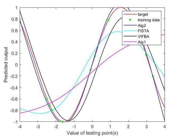
Figure 2. A regression of a sine function at the 130th iteration.

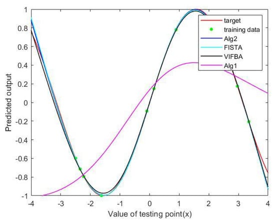
Figure 3. A regression of a sine function at the 3000th iteration.

4.2. Data Classification

In this experiment, we classify the type of Iris plants from Iris dataset created by Fisher [27]. As shown in Table 7, this dataset contains 3 classes of 50 instances and each sample contains four attributes.

Table 7. Iris dataset.

Class (50 Samples Each)	Attributes (in Centimeters)
Iris setosa Iris versicolor Iris virginica	sepal length sepal width petal length petal witdth

We also would like to thank https://archive.ics.uci.edu for providing the dataset.

With this dataset, we set sigmoid as an activation function, number of hidden nodes $M=100,$ and regularization parameter $\lambda =1\times {10}^{-5}.$ We use FISTA, VIFBA, Algorithms 4 and 5 as the training algorithm to estimate the optimal weight $\beta .$ The output data O of training and testing data are obtained by $O=\mathbf{H}\beta ,$ see Table 8 for more detail.

Table 8. Details about the classification of Iris dataset experiment.

Training set	Create the N × 1 training matrix S of number 1, 2 and 3 according to the training set and N is a number of training samples
	Create the N × 4 training attribute matrix R according to S and attribute data
Testing set	Create the M × 1 testing matrix T of number 1, 2 and 3 according to the testing set and M is a number of testing samples
	Create the M × 4 testing attribute matrix V according to T and attribute data
Learning process	Generate the hidden layer output matrix H1 of training attribute matrix R with 100 hidden nodes using sigmoid as the activation function
	Choose λ = 1 × 10−5 and formulate a convex minimization problem: $$\mathrm{Minimize}:{\Vert {\mathbf{H}}_1\beta -S\Vert }_2^2+\lambda {\Vert \beta \Vert }_1$$
	Find optimal weight β* of this problem using Algorithm 5 as a learning algorithm with certain number of iterations
Testing process	Calculate output O1 = H1β*
	Calculate number of correctly predicted samples between output O1 and training matrix S Generate the hidden layer output matrix H2 of testing attribute matrix V with 100 hidden nodes using sigmoid as the activation function
	Calculate output O2 = H2β*
	Calculate number of correctly predicted samples between output O2 and testing matrix T
	Calculate acc.train, acc.test, Average ACC, ERR%

Let the number 1, 2 and 3 represent Iris setosa, Iris versicolor and Iris virginica, respectively.

In the first experiment, we use the first 35 instances of each class as training data and the last 15 of each class as testing data, see Table 9 for detail.

Table 9. Training and testing sets of the Iris dataset.

Class	Training Data	Testing Data
Iris setosa	35	15
Iris versicolor	35	15
Iris virginica	35	15
Sum	105	45

The accuracy of the output data is calculated by:

$$\mathrm{accuracy}=\frac{\mathrm{correctly} \mathrm{predicted} \mathrm{data}}{\mathrm{all} \mathrm{data}}\times 100\%.$$

To compare the performance of FISTA, VIFBA, Algorithms 4 and 5, we choose parameters for each algorithm the same as in Table 4.

We first compare the accuracy of each method at the 700th iteration, and obtain the following results, as seen in Table 10.

Table 10. The performance of each algorithm at the 700th iteration.

	Iteration No.	Training Time	acc.train	acc.test
FISTA	700	0.0288	98.10	100
VIFBA	700	0.0416	98.10	100
Algorithm 4	700	0.3867	95.24	97.78
Algorithm 5	700	0.4172	99.05	100

As we see, from Table 10, Algorithm 5 obtains the highest accuracy at 700th iterations. We use acc.train and acc.test for the accuracy of the training data set and testing data set, respectively.

Next we compare each method with the stopping criteria as acc.train > 90 and acc.test > 90, the results can be seen in Table 11.

Table 11. The performance of each algorithm with the stopping criteria.

	Iteration No.	Training Time	acc.train	acc.test
FISTA	61	0.0038	91.43	91.11
VIFBA	32	0.0021	91.43	91.11
Algorithm 4	368	0.0816	90.48	91.11
Algorithm 5	65	0.0584	93.33	93.33

We observe from Table 11 that Algorithm 5 performs better than Algorithm 4.

In the next experiment, we use 10-fold stratified cross-validation to set up the training and testing data, see Table 12 for detail.

Table 12. Training and testing sets for 10-fold stratified cross-validation.

Class	Group 1–10
	Training Set	Testing Set
Iris Setosa	45	5
Iris versicolor	45	5
Iris virginica	45	5
Sum	135	15

We also use Average ACC and ERR${}_{\%}$ to evaluate the performance of each algorithm.

$${\displaystyle \mathrm{Average} \mathrm{ACC}=\sum _{i=1}^N\frac{x_i}{y_i}\times 100\%/N.}$$

where N is a number of sets considered during cross validation ($N=10$), $x_i$ a number of correctly predicted data at fold i and $y_i$ a number of all data at fold i.

Let err${}_{Lsum}$ = sum of errors in all 10 training sets, err${}_{Tsum}$ = sum of errors in all 10 testing sets, $Lsum=$ sum of all data in 10 training sets and $Tsum=$ sum of all data in 10 testing sets. Define

$${\mathrm{ERR}}_{\%}=({\mathrm{err}}_{L\%}+{\mathrm{err}}_{T\%})/2,$$

where err${}_{L\%}$ = $\frac{{\mathrm{err}}_{Lsum}}{Lsum}\times 100\%$, and err${}_{T\%}$ = $\frac{{\mathrm{err}}_{Tsum}}{Tsum}\times 100\%$.

We choose the same parameters as in Table 4. We compare the accuracy at the 1000th iteration of each fold, and obtain the following results, as seen in Table 13.

Table 13. The performance of each algorithm at the 1000th iteration with a 10-fold stratified cross-validation.

	FISTA		VIFBA		Algorithm 4		Algorithm 5
	acc.train	acc.test	acc.train	acc.test	acc.train	acc.test	acc.train	acc.test
Fold 1	97.78	100	97.78	100	97.78	100	97.78	100
Fold 2	99.26	93.33	99.26	93.33	99.26	93.33	98.52	93.33
Fold 3	97.78	100	97.78	100	95.56	100	98.52	100
Fold 4	99.26	93.33	99.26	93.33	97.04	93.33	97.78	86.67
Fold 5	98.52	100	98.52	100	97.78	100	98.52	100
Fold 6	98.52	100	98.52	100	98.52	100	98.52	100
Fold 7	98.52	86.67	98.52	86.67	98.52	73.33	98.52	93.33
Fold 8	98.52	100	98.52	100	98.52	100	98.52	100
Fold 9	98.52	100	97.78	100	97.04	100	97.78	100
Fold 10	98.52	100	98.52	100	97.78	100	97.78	100
Average Acc	98.52	97.333	98.446	97.333	97.778	96	98.222	97.333
ERR${}_{\%}$	2.074		2.112		3.111		2.223
Training time (sec.)	0.0413		0.0625		0.5673		0.7051

We observe from Table 13 that Algorithm 5 has higher average accuracy than Algorithm 4.

5. Conclusions

In this work, algorithms for solving a convex minimization problem (1) are studied. Many effective algorithms for solving this problem were proposed, most of them require a Lipschitz continuous assumption of $▿f.$ By combining a linesearch technique introduced by Cruz and Nghia [20], and an iterative method VIFBA by Verma et al. [19], we establish a new algorithm that does not require a Lipschitz continuous assumption of $▿f.$ As a result, it can be applied to solve problems in which Lipschitz constants do not exist, while VIFBA and FISTA cannot. Moreover, by viscosity approximation together with the inertial technique, our proposed algorithm has a better convergence behavior than Algorithm 4. A strong convergence of our proposed method is also proven under some control conditions that are weaker than that of VIFBA.

Our algorithm can be used to solve many real world problems such as image and signal processing, machine learning, especially regression and classification problems. To compare the performance of FISTA, VIFBA, Algorithm 4 and our proposed algorithm(Algorithm 5), we conduct numerical experiments on the latter problems. We observe from these experiments that Algorithms 4 and 5 take computational time longer than FISTA and VIFBA at the same number of iterations because the linesearch step (Linesearch 1) takes a long time to compute. In the experiments with the stopping criteria (Table 5 and Table 11), Algorithm 5 converges to a solution with a lower number of iterations than Algorithm 4 and hence performs better in terms of speed. We can also observe that Algorithm 5 performs decently in terms of accuracy, especially when compared with Algorithm 4.

For our future research, since FISTA performs better than Algorithm 5 in terms of speed, in order to compete with FISTA, we aim to find a new linesearch technique that takes less computational time than Linesearch 1 and hence decreases the computational time of Algorithm 5.

References

- Byrne, C. Iterative oblique projection onto convex subsets and the split feasibility problem. Inverse Probl. 2002, 18, 441–453. [Google Scholar] [CrossRef]
- Combettes, P.L.; Wajs, V. Signal recovery by proximal forward–backward splitting. Multiscale Model. Simul. 2005, 4, 1168–1200. [Google Scholar] [CrossRef]
- Combettes, P.L.; Pesquet, J.C. Proximal Splitting Methods in Signal Processing. In Fixed-Point Algorithms for Inverse Problems in Science and Engineering; Bauschke, H., Burachik, R., Combettes, P., Elser, V., Luke, D., Wolkowicz, H., Eds.; Springer: New York, NY, USA, 2011; pp. 185–212. [Google Scholar]
- Cholamjiak, P.; Shehu, Y. Inertial forward-backward splitting method in Banach spaces with application to compressed sensing. Appl. Math. 2019, 64, 409–435. [Google Scholar] [CrossRef]
- Szaleniec, M.; Tadeusiewicz, R.; Witkoa, M. How to select an optimal neural model of chemical reactivity? Neurocomputing 2008, 72, 241–256. [Google Scholar] [CrossRef]
- Szaleniec, J.; Wiatr, M.; Szaleniec, M.; Składzień, J.; Tomik, J.; Oleś, K.; Tadeusiewicz, R. Artificial neural network modelling of the results of tympanoplasty in chronic suppurative otitis media patients. Comput. Biol. Med. 2013, 43, 16–22. [Google Scholar] [CrossRef]
- Pławiak, P.; Abdar, M.; Acharya, U.R. Application of new deep genetic cascade ensemble of SVM classifiers to predict the Australian credit scoring. Appl. Soft Comput. 2019, 84, 105740. [Google Scholar] [CrossRef]
- Pławiak, P.; Abdar, M.; Pławiak, J.; Makarenkov, V.; Acharya, U.R. DGHNL: A new deep genetic hierarchical network of learners for prediction of credit scoring. Inf. Sci. 2020, 516, 401–418. [Google Scholar] [CrossRef]
- Lions, P.L.; Mercier, B. Splitting algorithms for the sum of two nonlinear operators. SIAM J. Numer. Anal. 1979, 16, 964–979. [Google Scholar] [CrossRef]
- Bussaban, L.; Suantai, S.; Kaewkhao, A. A parallel inertial S-iteration forward-backward algorithm for regression and classification problems. Carpathian J. Math. 2020, 36, 21–30. [Google Scholar]
- Moudafi, A.; Oliny, M. Convergence of a splitting inertial proximal method for monotone operators. J. Comput. Appl. Math. 2003, 155, 447–454. [Google Scholar] [CrossRef]
- Verma, M.; Shukla, K.K. A new accelerated proximal gradient technique for regularized multitask learning framework. Pattern Recogn. Lett. 2017, 95, 98–103. [Google Scholar] [CrossRef]
- Beck, A.; Teboulle, M. A fast iterative shrinkage-thresholding algorithm for linear inverse problems. SIAM J. Imaging Sci. 2009, 2, 183–202. [Google Scholar] [CrossRef]
- Liang, J.; Schonlieb, C.B. Improving fista: Faster, smarter and greedier. arXiv 2018, arXiv:1811.01430. [Google Scholar]
- Moudafi, A. Viscosity approximation method for fixed-points problems. J. Math. Anal. Appl. 2000, 241, 46–55. [Google Scholar] [CrossRef]
- Nakajo, K.; Takahashi, W. Strong convergence theorems for nonexpansive mappings and nonexpansive semigroups. J. Math. Anal. Appl. 2003, 279, 372–379. [Google Scholar] [CrossRef]
- Takahashi, W.; Zembayashi, K. Strong Convergence Theorem by a New Hybrid Method for Equilibrium Problems and Relatively Nonexpansive Mappings. Fixed Point Theory Appl. 2008, 2008, 528476. [Google Scholar] [CrossRef]
- Halpern, B. Fixed points of nonexpansive maps. Bull. Am. Math. Soc. 1967, 73, 957–961. [Google Scholar] [CrossRef]
- Verma, M.; Sahu, D.R.; Shukla, K.K. VAGA: A novel viscosity-based accelerated gradient algorithm. Appl. Intell. 2018, 48, 2613–2627. [Google Scholar] [CrossRef]
- Bello Cruz, J.Y.; Nghia, T.T. On the convergence of the forward-backward splitting method with linesearches. Optim. Methods Softw. 2016, 31, 1209–1238. [Google Scholar] [CrossRef]
- Burachik, R.S.; Iusem, A.N. Set-Valued Mappings and Enlargements of Monotone Operators; Springer: Berlin, Germany, 2008. [Google Scholar]
- Huang, Y.; Dong, Y. New properties of forward-backward splitting and a practical proximal-descent algorithm. Appl. Math. Comput. 2014, 237, 60–68. [Google Scholar] [CrossRef]
- Takahashi, W. Introduction to Nonlinear and Convex Analysis; Yokohama Publishers: Yokohama, Japan, 2009. [Google Scholar]
- Mainge, P.E. Strong convergence of projected subgradient methods for nonsmooth and nonstrictly convex minimization. Set-Valued Anal. 2008, 16, 899–912. [Google Scholar] [CrossRef]
- Xu, H.K. Another control condition in an iterative method for nonexpansive mappings. Bull. Austral. Math. Soc. 2002, 65, 109–113. [Google Scholar] [CrossRef]
- Tibshirani, R. Regression shrinkage and selection via the lasso. J. R. Stat. Soc. B Methodol. 1996, 58, 267–288. [Google Scholar] [CrossRef]
- Fisher, R.A. The use of multiple measurements in taxonomic problems. Ann. Eugen. 1936, 7, 179–188. [Google Scholar] [CrossRef]
© 2020 by the authors. Licensee MDPI, Basel, Switzerland. This article is an open access article distributed under the terms and conditions of the Creative Commons Attribution (CC BY) license (http://creativecommons.org/licenses/by/4.0/).