Outliers Detection Models in Shewhart Control Charts; an Application in Photolithography: A Semiconductor Manufacturing Industry

Abstract

Shewhart control charts with estimated control limits are widely used in practice. However, the estimated control limits are often affected by phase-I estimation errors. These estimation errors arise due to variation in the practitioner’s choice of sample size as well as the presence of outlying errors in phase-I. The unnecessary variation, due to outlying errors, disturbs the control limits implying a less efficient control chart in phase-II. In this study, we propose models based on Tukey and median absolute deviation outlier detectors for detecting the errors in phase-I. These two outlier detection models are as efficient and robust as they are distribution free. Using the Monte-Carlo simulation method, we study the estimation effect via the proposed outlier detection models on the Shewhart chart in the normal as well as non-normal environments. The performance evaluation is done through studying the run length properties namely average run length and standard deviation run length. The findings of the study show that the proposed design structures are more stable in the presence of outlier detectors and require less phase-I observation to stabilize the run-length properties. Finally, we implement the findings of the current study in the semiconductor manufacturing industry, where a real dataset is extracted from a photolithography process.

1. Introduction

The two salient tools of statistical process control (SPC) are memory and memory-less control charts. The memory-less control charts are most suitable for large shift, while the memory-control charts are used to monitor moderate and small shifts. The prominent form of memory-less control chart for location monitoring is the Shewhart $\overline{X}$ control chart. In general, control charts-irrespective of the magnitude they measure-operate in two phases: phase-I, the prospective stage from which the control limits are obtained; phase-II, where we monitor the process and correct the unnatural causes of variation whenever they occur (cf. [1]). In phase-I we estimate the control limits using the parameters of the process under study which, in reality, are seldom known. The amount of data employed in phase-I for estimating process parameters varies from one practitioner to the other. As a result, this variability affects the chart performance in the monitoring stage i.e., phase-II. (see for example [2,3,4,5,6]).

Furthermore, the amount of data employed in estimating the process parameters does affect the accuracy of the chart, as well as its limits. As we all know, the larger the sample size, the closer we are to the parameter. Therefore, increasing the sample size used for estimating the parameters should be the remedy to this shortcoming, but there is a limit to which we can increase sample sizes in real-life situations. As a result, the Shewhart chart, like any other chart, loses its performance and credibility. The depth of the loss depends on the efficacy of the parameter estimation and sample size employed in phase-I.

The presence of outlying/extreme values in the phase-I dataset can affect the performance of the control chart. The insufficiency of the phase-I estimates could be a result of extreme sample points in the sample, and not necessarily the size of the sample (see [5,7]). The easiest remedy for the extreme values is to drop such a sample and pick another one, but this is not appropriate for small sample data. Therefore, there is a need to screen the extreme values to improve the overall performance of the control chart.

Over the years, researchers have studied different types of robust outlier detection models in a series of control charts to enhance their performance. Examples include [8,9,10,11,12]. These outlier detectors require the data to be from normal distribution such as the Student-type and Grubbs-type detectors. However, for a non-normal dataset, the Tukey’s and median absolute deviation (MAD) outlier detection models are more accurate and robust since they are independent of mean and standard deviation. (see [13,14,15,16,17,18,19]). SPC is widely applied and implemented in various sectors; health, industrial, manufacturing and every service-rendering sector. Control charts, however, are most applied in manufacturing industry, with semiconductors as a case study. Semiconductor manufacturing processes are prone to high chances of assignable cause of variations, due to machine breakdown, multiple products, re-entrant flows, batching processes etc. [20]. Researchers have employed SPC in solving these recurring challenges in this industry (see [21,22,23,24]). The proposed charts in this study are applied in photolithography, a semiconductor manufacturing process.

In this article, we study the effects of parameter estimation on the Shewhart $\overline{X}$ chart for normal and non-normal environments. We also study the effect of outliers on the reliability of the control charts and the process parameters are estimated. Furthermore, we propose non-parametric outlier detectors, namely: the robust Tukey and MAD outlier detection models in designing the basic control chart structure. A fair comparison between the two-outlier detection models is also made. We achieve all of these using average run length (ARL) and standard deviation run length (SDRL) as the performance measures.

The remainder of this article is as follows: the next Section entails the methodologies employed for the study; briefing the overview of the Shewhart $\overline{X}$ control chart when the parameters are known and unknown, alongside the performance measure properties adopted in this study; the variability in Shewhart chart performance due to phase-I estimation; a scenario for the presence of outliers in the design structure of Shewhart chart, and its effect; incorporating the Turkey and MAD outlier detection models in the design structure of the Shewhart chart as remedies for rectifying the presence of outliers; Section 3 gives a concise and precise description of the simulation results. In Section 4, a detailed comparison of the results is presented; while Section 5 provides an illustrative example with a real life dataset; finally a concluding remark and future recommendations are given in Section 6.

2. Methodology

In this section, we give details of the Shewhart control chart for normal and non-normal environments. The known and unknown parameter scenarios, the practitioner–practitioner variation in the estimation stage, the presence of outliers/extreme values in the estimation sample, and incorporating some outlier detection models in the Shewhart chart are all discussed in the following subsections.

2.1. Overview of the Shewhart Control Chart

Let $Y_{ij}$ $i=1, 2, \dots ,n$ and $j=1, 2, \dots$ represent a $i$th observation from $j$th sample of an ongoing (continuous) process. Further $Y_{ij}$ follows a normal distribution with mean ${\mu }_0+\delta {\sigma }_0$ and variance ${\sigma }_0{}^2$ i.e., $Y_{ij} ~ N\left({\mu }_0+\delta {\sigma }_0, {\sigma }_0{}^2\right)$. The process is said to be in the in-control (IC) state if$\delta =0$, and out-of-control (OoC) otherwise. A default Shewhart set-up monitors a process by plotting the sample mean (${\overline{Y}}_i=1/n{{\displaystyle \sum }}_{j=1}^n{Y}_{ij}$) of $Y_{ij}$ against the following control chart limits.

$$\mathrm{UCL}={\mu }_0+L\frac{{\sigma }_0}{\sqrt{n}} , \mathrm{LCL}={\mu }_0-L\frac{{\sigma }_0}{\sqrt{n}}$$

(1)

where UCL and LCL denote the upper and lower control limits, respectively. Limits in (1) are useful when the parameters (${\mu }_0$ and${\sigma }_0{}^2$) of the process are known. However, when they are unknown, their respective unbiased estimators from the phase-I are used, and the resulting control chart structures will be in estimated form.

For phase-I, let$Y_{il}$ represents $i$th observation from $l$th random sample $\forall i=1, 2, 3, \dots , n$ and $l=1, 2, 3, \dots , m$, regarded to be under statistically IC state. It is good to mention here that the choice of $m$ and $n$ varies from one practitioner-to another. Therefore, it affects the accuracy of the control limits implying an influenced ARL in phase-II. The unbiased estimators for the parameters $\mu$ and $\sigma$ of an IC process are defined as:

$$\begin{array}{c}{\widehat{\mu }}_0=\left(1/m\right){{\displaystyle \sum }}_{l=1}^m{\overline{Y}}_l\\ {\widehat{\sigma }}_0=\left(1/m{C}_4\right){{\displaystyle \sum }}_{l=1}^m{S}_l\end{array}$$

(2)

where ${\overline{Y}}_l=\frac{{{\displaystyle \sum }}_{l=1}^n{Y}_{il}}{n}$, $S_l=\sqrt{\frac{{{\displaystyle \sum }}_{i=1}^n{\left(Y_{il}-{\overline{Y}}_l\right)}^2}{n-1}}$ and $c_4=\frac{\sqrt{2/\left(n-1\right)}\mathsf{\Gamma }\left(n/2\right)}{\mathsf{\Gamma }\left[\left(n-1\right)/2\right]}$ is the bias correction constant. Subsequently, the resulting control limits in (1) are modified to the following:

$$\widehat{\mathrm{UCL}}=\frac{{{\displaystyle \sum }}_{l=1}^m{\overline{Y}}_l}{m}+\widehat{L}\frac{{{\displaystyle \sum }}_{l=1}^m{S}_l}{m{C}_4\sqrt{n}} , \widehat{\mathrm{LCL}}=\frac{{{\displaystyle \sum }}_{l=1}^m{\overline{Y}}_l}{m}-\widehat{L}\frac{{{\displaystyle \sum }}_{l=1}^m{S}_l}{m{C}_4\sqrt{n}}$$

(3)

In phase-II, ${\overline{Y}}_l$s are plotted against the control limits in (3) and the chart is said to have given an OoC signal if any value of ${\overline{Y}}_l$ is plotted outside the limits. Here, the sample number at which the statistic is plotted outside the limits is recorded as run length (RL). RL is an important variable in measuring the performance of control charts in general, and the Shewhart is not an exception. The most widely used property of RL is ARL, which is the average number of samples observed before the chart sends an OoC signal. Mathematically, $\mathrm{ARL}={{\displaystyle \sum }}_{k=1}^{s}R{L}_k/s$ where s is the number of RLs recorded. In addition to ARL, standard deviation of the RL (SDRL) gives more information about the behavior of the RL variable in evaluating the performance of a control chart. Furthermore, the ARL is of two types i.e., the IC ARL, denoted as $\mathrm{AR}{\mathrm{L}}_0$ and the OoC ARL, referred to as$\mathrm{AR}{\mathrm{L}}_1$. $\mathrm{AR}{\mathrm{L}}_0$ is expected to be sufficiently large enough to avoid false alarms. On the other hand, $\mathrm{AR}{\mathrm{L}}_1$ is anticipated to be sufficiently small to enable the process to send a signal as soon as there is a shift in the process parameter(s).

2.2. Variability in the Shewhart Chart Performance

In this section, we explain the effect of the practitioner to practitioner variability on the Shewhart chart, both in normal and non-normal distribution, by using the Monte Carlo simulation approach. See ([25,26,27,28,29]) for more information about the effect of sample size and practitioners’ variability. To achieve this aim, we develop an algorithm in R programing language to simulate the Shewhart chart environment, using the standard Shewhart chart as our benchmark and reference point. The $\overline{X}$ chart has a control limits width determinant $L$ that influences RL properties. We use the standard $L=3$, that corresponds to the$\mathrm{AR}{\mathrm{L}}_0=370$ (see [1] for more details). Without any loss of generality, we generate random samples from a standard normal distribution $N\left(\mu =0, \sigma =1\right)$, each of sample size$n=5$, assuming the process parameters are known. While for the non-normal distribution, we considered the t-distribution with degrees of freedom $v=5, 25,$ and$100$. Since all the three categories of $v$ exhibit the same pattern, we report only the results for$v=100$. In both environments, normal and t-distributions, we set up the chart limits as given in Equation (1) and plot the sample means against the UCL and LCL. As soon as a value of ${\overline{ Y}}_j$ is plotted outside the limits, RL is recorded and saved. The process is iterated ${10}^5$ times to get ARL and SDRL.

For the unknown parameters, we estimate the parameter from phase-I. The number of samples employed for the estimation differs from on practitioner to another and so does the accuracy of the charts in phase-II. To depict that, we estimated both ${\mu }_0$ and${\sigma }_0$ from different number of in-control phase-I samples i.e., $m=25, 50, 100, 250, 500$ and 1000 each of sample size$n=5$. The estimated parameters ${\widehat{\mu }}_0$ and${\widehat{\sigma }}_0$ from the phase-I IC stage are, therefore, used in the same algorithm instead of ${\mu }_0$ and${\sigma }_0$ respectively. Subsequently the parameter $L$, changes as the amount of phase-I samples changes. The corresponding $L’$s for the different$m^{\prime }\mathrm{s}$ are $L=2.962, 2.983, 2.9925, 2.997, 2.999,$ and $3$ respectively for the normal distribution, and $L=2.974, 2.995, 3.005, 3.010, 3.012,$ and $3.012$ respectively for the t-distribution of $v=100$. These $L$’s are determined through simulations to obtain$\mathrm{AR}{\mathrm{L}}_0=370$. We carry out the simulation with different level of shifts $\delta$ ranging from 0 to 5 i.e., $\delta \in \left(0,0.5,5\right)$, as shown in

Table 1. Average run length (ARL) of the Shewhart chart with estimated parameters for standard normal and t (v = 100) distributions.

ARL	Standard Normal Distribution						T-Distribution v = 100
ẟ/m	25	50	100	250	500	1000	25	50	100	250	500	1000
0	370.93	369.66	370.43	369.09	371.10	370.98	370.67	370.00	369.58	370.89	369.63	370.00
0.5	190.76	173.92	165.35	159.25	157.00	156.54	194.06	177.76	167.85	161.75	160.48	159.04
1	53.91	48.74	46.37	44.73	44.41	44.21	55.14	50.13	47.75	46.26	46.02	45.32
1.5	17.19	16.05	15.52	15.20	15.09	15.04	17.70	16.53	16.06	15.65	15.65	15.52
2	6.87	6.59	6.46	6.35	6.33	6.33	7.05	6.80	6.65	6.57	6.54	6.57
2.5	3.40	3.33	3.29	3.26	3.25	3.25	3.52	3.44	3.40	3.36	3.35	3.35
3	2.05	2.03	2.02	2.01	2.00	2.00	2.10	2.08	2.06	2.06	2.05	2.05
3.5	1.47	1.46	1.45	1.45	1.45	1.45	1.50	1.49	1.48	1.48	1.48	1.47
4	1.20	1.19	1.19	1.19	1.19	1.19	1.21	1.21	1.21	1.21	1.20	1.20
4.5	1.08	1.08	1.07	1.07	1.07	1.07	1.09	1.08	1.08	1.08	1.08	1.08
5	1.03	1.02	1.02	1.02	1.02	1.02	1.03	1.03	1.03	1.03	1.03	1.03
L	2.962	2.983	2.9925	2.997	2.999	3	2.974	2.995	3.005	3.010	3.012	3.012

and

Table 2. Standard deviation of the run length (SDRL) of the Shewhart chart with estimated parameters for standard normal and t (v = 100) distributions.

SDRL	Standard Normal Distribution						T-Distribution v = 100
ẟ/m	25	50	100	250	500	1000	25	50	100	250	500	1000
0	601.54	473.20	420.75	387.76	379.99	375.44	601.69	468.55	416.69	389.69	376.91	373.30
0.5	333.88	232.92	193.19	169.15	161.43	158.10	340.19	241.98	197.21	172.49	164.11	160.46
1	88.35	61.71	52.00	46.39	45.00	44.24	91.10	64.04	53.93	47.96	46.61	45.29
1.5	24.05	18.52	16.40	15.20	14.85	14.67	25.00	19.21	16.92	15.71	15.33	15.20
2	8.24	6.88	6.32	5.97	5.90	5.85	8.73	7.10	6.48	6.22	6.11	6.11
2.5	3.40	3.04	2.86	2.76	2.72	2.71	3.60	3.16	2.99	2.86	2.84	2.83
3	1.66	1.54	1.48	1.44	1.43	1.42	1.70	1.59	1.54	1.49	1.48	1.47
3.5	0.90	0.85	0.83	0.81	0.81	0.81	0.94	0.89	0.86	0.84	0.84	0.84
4	0.51	0.49	0.48	0.48	0.48	0.48	0.54	0.51	0.51	0.50	0.50	0.50
4.5	0.30	0.29	0.28	0.28	0.28	0.28	0.32	0.31	0.30	0.29	0.29	0.29
5	0.17	0.16	0.16	0.16	0.16	0.16	0.18	0.17	0.17	0.17	0.17	0.17
L	2.962	2.983	2.9925	2.997	2.999	3	2.974	2.995	3.005	3.010	3.012	3.012

.

2.3. Presence of Outliers in the Shewhart Chart with Estimated Parameters

Although the estimation of the unknown parameters in phase-I samples plays its role on the efficiency of the control chart in phase-II. The drop in the efficacy of the chart performance is not limited to this fact alone, rather it extends to presence of outlying/extreme values in the phase-I samples.

In this Section, we study the effect of outliers in the phase-I samples on the performance and accuracy of the Shewhart chart. Here, through Monte Carlo simulation, we generate the $m$ phase-I samples from a mixture distribution i.e., $\left(1-\alpha \right)100\%$ from assumed (normal or t-distribution) and the remaining $\alpha 100\%$ from a chi-square distribution with $n$ degrees of freedom denoted by${\chi }_{\left(n\right)}^2$. Subsequently, the estimated parameters emerging from the $m$ samples have an extreme values effect on the control chart in phase-II. That is, each observation of the phase-I sample is generated from the following expression:

$$\begin{array}{c}\left(1-\alpha \right)N\left(\mu ,{\sigma }^2\right)+\alpha \left[N\left(\mu ,{\sigma }^2\right)+w {\chi }_{\left(n\right)}^2\right] or\\ \left(1-\alpha \right)t\left(v\right)+\alpha \left[t\left(v\right)+w {\chi }_{\left(n\right)}^2\right]\end{array}$$

(4)

where $\alpha >0$, is the probability of having a multiple of ${\chi }_{\left(n\right)}^2$ added to the assumed distribution, serving as the outliers in the samples. In addition,$w\ge 1$ is the magnitude of the outlier. We develop an algorithm from the R language, similar to that in Section 2.2, but the samples are from the environment described in (4). We set$\mu =0, {\sigma }^2=1, v=100,w=3$, and$\alpha ϵ\left[0,0.01\right]$. We design the Shewhart chart using the same parameters $L$ and $m$ as in Section 2.2.

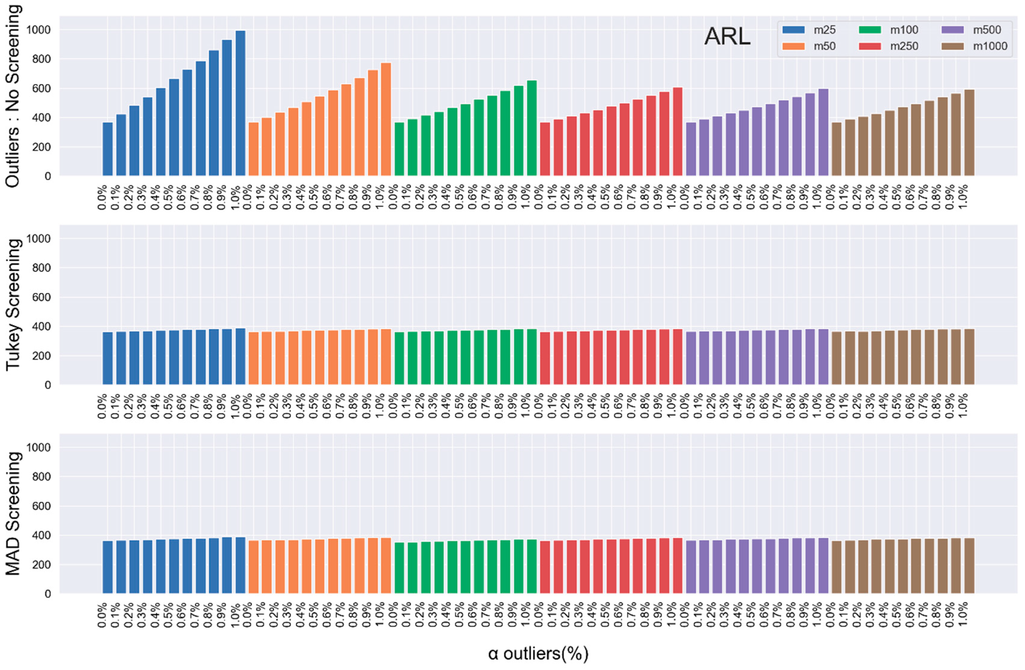
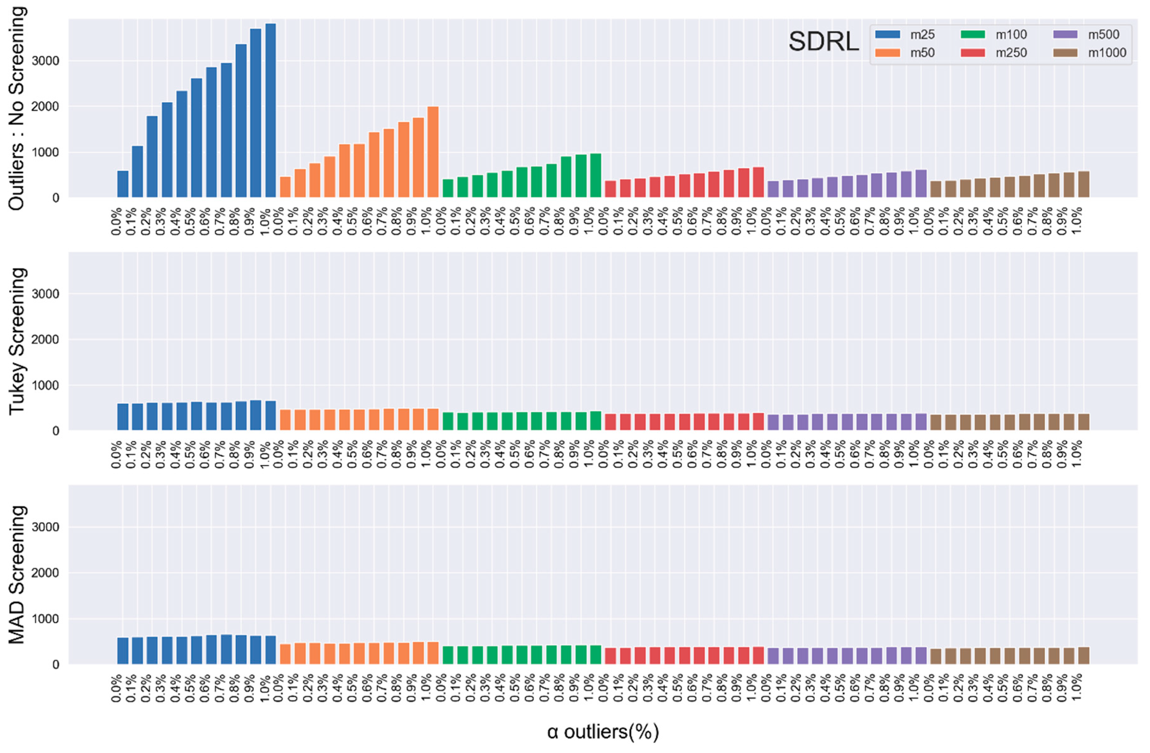
In general, the pattern exhibited by the RL properties implies the following:

• Increasing the$m$ phase-I samples in the presence of outliers, gets the$\mathrm{AR}{\mathrm{L}}_0$’s closer to the theoretical values.
• Reducing the value of$\alpha$, the percentage of outliers present in the$m$ samples also brings the$\mathrm{AR}{\mathrm{L}}_0$’s closer to the theoretical values.

Unfortunately, neither of the two suggested remedies is practicable in real life. Thus, we propose outliers detecting structures through the robust Turkey and MAD detection models.

2.4. Shewhart Chart with Outlier Detection Models

In the section, we propose two outlier-detecting models as remedy to the issues raised in Section 2.2 and Section 2.3. The Tukey and the MAD model-based Shewhart charts. Their procedures applied in parallel to the Shewhart chart are described in the sub sections below:

2.4.1. The Tukey Shewhart Control Chart

For the phase-I samples, $\tilde{Y}$ be the median of all $m\times n$ observations. For any observation $y_o$ if$\left|y_o-\tilde{Y}\right|>p\times IQR$, then $y_o$ is declared an outlier. Here $IQR=Q_3-Q_1$ is the inter-quartile range of the sample. $Q_3$ and $Q_1$ are the third and first quartiles, respectively, of all $m\times n$ phase-I observations. The constant $p$ on the other hand is the confidence factor of the Tukey’s detector, commonly chosen between 1.5 and 3.0. The confidence factor should be carefully chosen, and not too small, to avoid over detection. Also it should not be too large, to prevent under detection [18]. In this study, we choose$p=2.2$. Applying the same algorithm, parameters and limits employed in Section 2.2, we incorporate the Tukey outlier-detector model on the phase-I samples to screen out the extreme values present there in. Then we compute the IC ARL and SDRL values for the Shewhart chart based on the Tukey model in phase-II, when the parameters are estimated.

2.4.2. The Median Absolute Deviation (MAD) Shewhart Control Chart

We define median absolute deviation (MAD) as the deviation of the dataset about the median as$\mathrm{MAD}=median\left(\left|Y_{il}-\tilde{Y}\right|\right)/0.6574$. Then it follows, that any observation $y_{o }$ from the sample that falls outside the expression$\widetilde{ Y}\pm b\ast \mathrm{MAD}$, is declared an outlier. Here $b$ is the outlier detecting constant and chosen $3.642$ so that the percentage of screening by MAD is the same as Tukey. This has been done to keep the comparison between two outlier detectors valid [19].

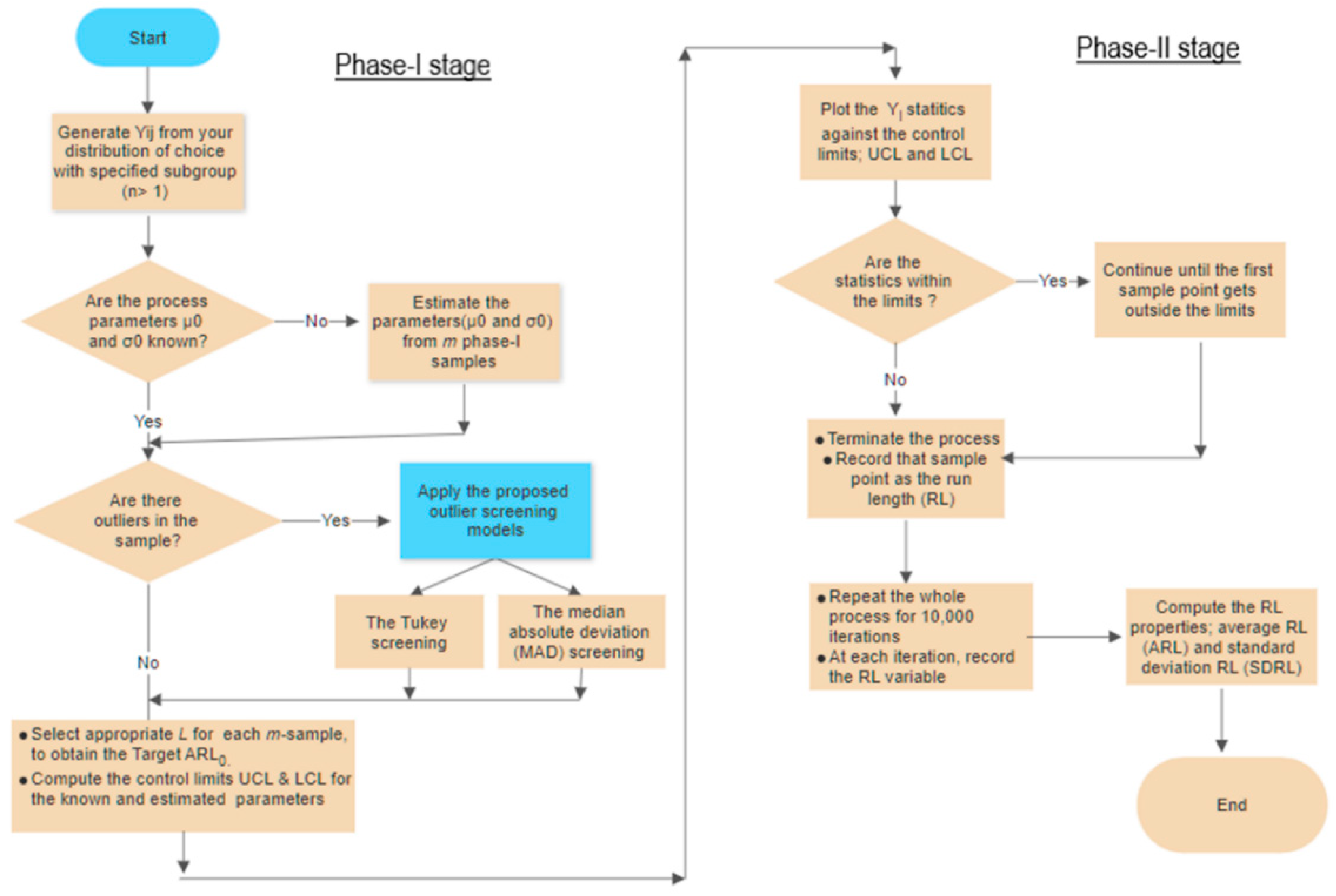
Furthermore, it is worth distinguishing between outlying and OoC sample points. The former emerges from $m$phase-I samples, which are used to construct the control limits for the monitoring stage; phase-II; while the latter are the sample points that fall beyond the control limits in phase-II. Therefore, the presence of outlying sample points in phase-I leads to wider control limits, rendering the control charts less effective. A flowchart summarizing the procedure is depicted in Figure 1.

3. Results

In this section, we provide the results of the methodologies discussed in Section 2. These results are presented in three folds, so is the discussion in the next section.

3.1. Practitioners’ Estimation Variability

Here, through the simulation results of the algorithm explained in Section 2.2, we observe the variability that appears in the Shewhart control chart due to different choices of sample size$m$, amongst practitioners. Table 1 and Table 2 depict the Shewhart chart whose parameters, both mean and variance, are estimated from $m$ phase-I samples for both normal and non-normal distributions. It is evident from the result, the effect of parameter estimation on the performance of the chart. The$\mathrm{AR}{\mathrm{L}}_0$s when$\delta =0$, are clustering around the target $370$ with their respective $L$’s. However, when$\delta \ne 0$, we observe that the smaller $m$ becomes, the less effective the Shewhart chart performance. The$\mathrm{AR}{\mathrm{L}}_1$’s are expected to be sufficiently small in order to detect any drift in the ongoing process, but as $m$ gets smaller,$\mathrm{AR}{\mathrm{L}}_1$’s get bigger. Which implies the chart is less sensitive in identifying the presence of shifts in the ongoing process early enough. Another noticeable effect of the parameter estimation on the Shewhart chart is the decrement in the limits L, as $m$ reduces. This should be recorded as an edge if the corresponding phase-II charts detects shift earlier than when the parameters are known.

3.2. Effect of Outliers on the Shewhart Control Charts

In

Table 3. ARL of the Shewhart chart in the presence of outliers with estimated parameters for standard normal and t (v = 100) distributions.

ARL	Standard Normal Distribution						T-Distribution v = 100
α/m	25	50	100	250	500	1000	25	50	100	250	500	1000
0	371.20	369.51	370.29	369.59	370.72	370.85	370.65	369.57	369.28	370.85	369.11	370.87
0.001	424.76	401.49	392.98	389.92	388.74	389.13	418.21	394.60	386.19	385.76	385.04	381.04
0.002	484.38	435.14	417.35	410.86	409.61	408.88	478.03	424.90	408.83	405.04	403.56	398.94
0.003	540.09	469.66	440.42	431.91	429.47	428.70	534.47	458.93	435.77	424.67	424.75	422.44
0.004	602.97	507.51	469.33	452.76	450.30	449.72	587.12	500.66	457.98	443.64	444.15	437.50
0.005	664.58	545.85	494.67	477.03	471.98	471.09	650.79	528.62	489.31	469.04	461.71	461.22
0.006	731.55	588.72	525.81	500.69	495.46	493.34	718.10	569.85	512.77	491.40	486.42	481.51
0.007	788.48	629.88	554.41	525.13	519.74	516.88	758.54	604.64	539.10	514.95	509.78	504.97
0.008	861.51	673.43	586.11	551.83	544.06	541.56	837.89	652.55	578.41	541.64	531.29	528.75
0.009	931.14	726.12	618.88	579.38	569.55	565.85	916.99	693.94	606.71	568.85	560.07	552.75
0.01	996.35	773.78	654.18	607.70	596.56	592.55	953.61	745.34	634.00	593.84	586.09	575.08
L	2.962	2.983	2.9925	2.997	2.999	3	2.974	2.995	3.005	3.010	3.012	3.012

and

Table 4. SDRL of the Shewhart chart in the presence of outliers with estimated parameters for standard normal and t (v = 100) distributions.

SDRL	Standard Normal Distribution						T-Distribution v = 100
α/m	25	50	100	250	500	1000	25	50	100	250	500	1000
0	607.93	473.75	419.35	388.27	379.67	375.44	595.89	468.00	418.16	382.43	375.42	369.72
0.001	1238.32	664.83	467.76	414.51	400.57	394.71	1150.79	635.34	463.74	411.63	395.24	385.68
0.002	1704.83	838.46	515.41	441.77	423.19	415.18	1802.06	760.16	508.22	433.04	416.23	406.03
0.003	2041.64	991.95	568.33	468.17	446.51	436.26	2096.30	913.63	558.95	460.42	441.81	431.04
0.004	2410.92	1176.26	630.64	497.30	469.60	459.66	2354.27	1184.84	606.26	486.65	462.63	447.94
0.005	2689.45	1294.24	687.44	528.00	494.90	481.60	2626.16	1192.76	683.26	517.24	485.89	473.05
0.006	2994.88	1502.07	756.39	559.42	521.35	505.08	2871.17	1449.52	699.03	546.74	512.57	494.30
0.007	3193.80	1637.48	822.18	592.02	549.29	530.76	2956.37	1514.95	757.01	573.97	540.59	519.76
0.008	3480.50	1799.40	888.29	627.68	578.43	557.35	3370.66	1664.42	912.65	618.19	564.09	544.14
0.009	3772.38	1994.86	959.76	664.49	607.34	582.18	3703.48	1766.87	955.78	655.56	594.72	571.46
0.01	4012.72	2139.41	1028.74	702.52	638.62	612.00	3823.24	2009.14	980.24	685.94	628.22	591.55
L	2.962	2.983	2.9925	2.997	2.999	3	2.974	2.995	3.005	3.010	3.012	3.012

, we present the simulation results of environment (4) discussed in Section 2.3. From these results, the gross impact of outliers in the phase-I samples on the performance of the Shewhart chart cannot be over emphasized. Having seen the pattern of the IC and OoC RL properties in Table 1 and Table 2, in order to save space, we restrict the performance evaluation to the IC RL properties. That is, considering the case when$\delta =0$ only. From Table 3 and Table 4, when$\alpha =0$, in the absence of outlier, the$\mathrm{AR}{\mathrm{L}}_0$’s are clustering around its target$370$, irrespective of the amount of phase-I sample$m$. However, when$\alpha >0$, the$\mathrm{AR}{\mathrm{L}}_0$’s deviate from the target, vigorously. As the amount of phase-I samples$m$ reduces, and the percentage of outliers present in the samples$\alpha$ increases, the more the$\mathrm{AR}{\mathrm{L}}_0$’s deviate from the target. Similarly the pattern of the SDRL, even more.

3.3. Improvement of Tukey and MAD Outlier Detection Models on Shewhart Chart Performance

While incorporating the procedures in Section 2.4.1 and Section 2.4.2, the simulation results are presented in

Table 5. ARL of the Shewhart chart with Tukey outlier detection for standard normal and t (v = 100) distributions.

ARL	Standard Normal Distribution						T-Distribution v = 100
α/m	25	50	100	250	500	1000	25	50	100	250	500	1000
0	363.24	363.44	364.17	364.36	365.34	366.80	358.67	358.71	357.97	358.10	359.64	357.52
0.001	365.71	366.33	366.48	366.83	367.56	368.22	361.59	360.26	357.98	362.04	359.85	360.39
0.002	367.81	367.30	368.51	368.71	369.89	366.67	364.59	363.25	359.73	359.63	363.42	361.61
0.003	370.30	370.04	370.91	371.14	370.90	371.03	365.85	365.75	364.12	361.29	362.85	362.73
0.004	372.35	371.48	372.44	372.76	372.72	374.13	368.84	365.44	365.73	365.64	365.87	366.25
0.005	376.13	374.05	374.49	373.95	375.73	377.23	370.27	368.13	366.95	366.59	366.89	367.05
0.006	377.97	376.06	376.96	376.61	376.88	379.44	372.27	368.44	368.28	371.20	371.40	370.77
0.007	380.13	378.38	379.03	378.98	379.15	379.44	374.78	372.44	371.54	370.82	370.45	371.76
0.008	383.48	380.17	380.51	380.63	380.56	381.29	378.04	372.69	372.06	373.31	376.35	374.45
0.009	386.35	383.02	383.50	382.73	383.29	382.84	377.58	374.74	371.66	375.88	375.09	372.29
0.01	388.82	384.62	385.57	383.80	384.95	386.39	381.84	377.80	378.17	377.29	378.48	374.09
L	2.962	2.983	2.9925	2.997	2.999	3	2.974	2.995	3.005	3.010	3.012	3.012

,

Table 6. SDRL of the Shewhart chart with Tukey outlier detection for standard normal and t (v = 100) distributions.

SDRL	Standard Normal Distribution						T-Distribution v = 100
α/m	25	50	100	250	500	1000	25	50	100	250	500	1000
0	596.32	468.02	414.04	383.16	374.68	368.66	607.33	467.10	411.17	377.81	369.81	360.34
0.001	600.30	472.43	417.55	385.96	377.25	372.35	612.79	467.20	406.53	380.03	366.57	366.34
0.002	607.28	476.91	419.54	388.33	379.39	371.64	627.84	471.38	410.10	376.44	372.50	365.67
0.003	615.99	477.95	422.41	389.95	380.10	375.45	617.88	474.03	415.42	378.88	374.34	366.23
0.004	615.39	481.58	423.16	392.96	382.24	377.77	636.02	476.02	416.09	385.14	377.04	371.24
0.005	625.95	486.00	427.29	393.54	385.71	380.37	650.31	480.25	420.69	387.36	377.24	370.45
0.006	636.60	488.82	430.22	396.23	386.61	383.77	637.39	483.89	423.95	390.68	383.17	376.49
0.007	646.05	490.89	433.11	399.86	389.30	384.98	630.84	488.73	429.10	390.52	381.42	377.88
0.008	656.27	496.12	435.44	400.84	391.44	385.54	654.64	489.53	430.19	391.87	386.60	378.02
0.009	654.98	500.43	439.24	403.24	393.19	387.01	675.27	499.78	423.47	395.23	385.19	380.11
0.01	669.83	502.93	441.89	404.61	395.16	390.51	672.71	493.77	436.38	399.23	390.17	380.26
L	2.962	2.983	2.9925	2.997	2.999	3	2.974	2.995	3.005	3.010	3.012	3.012

,

Table 7. ARL of the Shewhart chart with median absolute deviation (MAD) outlier detection for standard normal and t (v = 100) distributions.

ARL	Standard Normal Distribution						T-Distribution v = 100
α/m	25	50	100	250	500	1000	25	50	100	250	500	1000
0	363.24	363.44	364.17	364.36	365.34	366.80	358.67	358.71	357.97	358.10	359.64	357.52
0.001	365.71	366.33	366.48	366.83	367.56	368.22	361.59	360.26	357.98	362.04	359.85	360.39
0.002	367.81	367.30	368.51	368.71	369.89	366.67	364.59	363.25	359.73	359.63	363.42	361.61
0.003	370.30	370.04	370.91	371.14	370.90	371.03	365.85	365.75	364.12	361.29	362.85	362.73
0.004	372.35	371.48	372.44	372.76	372.72	374.13	368.84	365.44	365.73	365.64	365.87	366.25
0.005	376.13	374.05	374.49	373.95	375.73	377.23	370.27	368.13	366.95	366.59	366.89	367.05
0.006	377.97	376.06	376.96	376.61	376.88	379.44	372.27	368.44	368.28	371.20	371.40	370.77
0.007	380.13	378.38	379.03	378.98	379.15	379.44	374.78	372.44	371.54	370.82	370.45	371.76
0.008	383.48	380.17	380.51	380.63	380.56	381.29	378.04	372.69	372.06	373.31	376.35	374.45
0.009	386.35	383.02	383.50	382.73	383.29	382.84	377.58	374.74	371.66	375.88	375.09	372.29
0.01	388.82	384.62	385.57	383.80	384.95	386.39	381.84	377.80	378.17	377.29	378.48	374.09
L	2.962	2.983	2.9925	2.997	2.999	3	2.974	2.995	3.005	3.010	3.012	3.012

and

Table 8. SDRL of the Shewhart chart with MAD outlier detection for standard normal and t (v = 100) distributions.

SDRL	Standard Normal Distribution						T-Distribution v = 100
α/m	25	50	100	250	500	1000	25	50	100	250	500	1000
0	596.32	468.02	414.04	383.16	374.68	368.66	607.33	467.10	411.17	377.81	369.81	360.34
0.001	600.30	472.43	417.55	385.96	377.25	372.35	612.79	467.20	406.53	380.03	366.57	366.34
0.002	607.28	476.91	419.54	388.33	379.39	371.64	627.84	471.38	410.10	376.44	372.50	365.67
0.003	615.99	477.95	422.41	389.95	380.10	375.45	617.88	474.03	415.42	378.88	374.34	366.23
0.004	615.39	481.58	423.16	392.96	382.24	377.77	636.02	476.02	416.09	385.14	377.04	371.24
0.005	625.95	486.00	427.29	393.54	385.71	380.37	650.31	480.25	420.69	387.36	377.24	370.45
0.006	636.60	488.82	430.22	396.23	386.61	383.77	637.39	483.89	423.95	390.68	383.17	376.49
0.007	646.05	490.89	433.11	399.86	389.30	384.98	630.84	488.73	429.10	390.52	381.42	377.88
0.008	656.27	496.12	435.44	400.84	391.44	385.54	654.64	489.53	430.19	391.87	386.60	378.02
0.009	654.98	500.43	439.24	403.24	393.19	387.01	675.27	499.78	423.47	395.23	385.19	380.11
0.01	669.83	502.93	441.89	404.61	395.16	390.51	672.71	493.77	436.38	399.23	390.17	380.26
L	2.962	2.983	2.9925	2.997	2.999	3	2.974	2.995	3.005	3.010	3.012	3.012

respectively. Table 5 and Table 7 represents the ARL result for Tukey and MAD outlier detection models respectively, as Table 6 and Table 8 are the corresponding SDRL results. The effect of these detection models are noticed as ARLs and SDRLs are closer to when there is an absence of outliers or even better.

For better visuals of the results, we depict the ARL results (Table 3, Table 5 and Table 7) in Figure 2 and Figure 3 and the SDRL results (Table 4, Table 6 and Table 8) in Figure 4 and Figure 5.

4. Discussion

We summarize the findings of the study under the following subsections: (a) parameter estimation effect on the Shewhart control chart, (b) effect of outliers on Shewhart $\overline{X}$ chart performance, and (c) improvement of outliers screening models on the Shewhart $\overline{X}$ chart performance. Through the discussion, we use the run length properties as a yardstick for measuring the performance of the charts.

4.1. Parameter Estimation Effect on the Shewhart $\overline{X}$ Control Chart

Theoretically, when the Shewhart charts parameters are known, the limit $L$ corresponding to the IC $\mathrm{AR}{\mathrm{L}}_0=370$ is$L=3$. When the parameters are estimated from phase-I samples, the first effect of the estimation is the change in$L$. The control limit $L$ deviates from its theoretical value as much as the sample size $m$ reduces. That implies, the smaller the sample size$m$, the farther the control limit from the theoretical value. This is noticeable in Table 1 and Table 2, as $L$ changes as the sample size does. We compute$L$s based on 100,000 iterations of simulation. Secondly, in the introduction of shifts, which makes the process OC, the RL properties values of the estimated parameters are bigger than the theoretical values. This indicates that the chart with estimated parameters are slower in detecting shifts in the process as compared to the chart with known parameters. For instance, (cf. Table 1 and Table 2), with$m=1000$,$\delta =0.5$ the resulting $\mathrm{AR}{\mathrm{L}}_1$ and $\mathrm{SDR}{\mathrm{L}}_1$ are $156.42$ and $158.84$ for normal distribution and $150.92$ and $160.46$ for t-distribution respectively. However, with$m=25$,$\delta =0.5$ $\mathrm{AR}{\mathrm{L}}_1$ and $\mathrm{SDR}{\mathrm{L}}_1$ are $190.12$ and $333.88$ for normal distribution and $194.06$ and $340.19$ for t-distribution respectively.

4.2. Effect of Outliers on Shewhart $\overline{X}$ Control Chart performance

Haven noticed the effect of parameter estimation on Shewhart chart performance; one major cause could be the presence of outliers in the dataset. The results in Table 3 and Table 4 prove that extreme values in the sample causes great havoc to the performance of the process. As discussed earlier in Section 4, $\alpha =0$ indicates absence of outliers, and the presence of outliers if otherwise. We observe jumps in the values of IC ARL and SDRL from Table 3 and Table 4. With different combinations of $\alpha$ and$m$, we say the bigger the value of $\alpha$ and the smaller the value of$m$, the gross the effect of the outliers on the chart. Take for instance, in the normal environment, the ARL and SDRL values of just 1% of outliers $\left(\alpha =0.01\right)$ for when $m=1000$ as against when$m=25$. It shocks to see the ARL and SDRL jumped from $592.55$ and $612.00$ to $996.3$ and $4012.72$ respectively. However, in the t-distribution, ARL and SDRL values of 1% of outliers $\left(\alpha =0.01\right)$ for when $m=1000$ as against when$m=25$, are $575.08$ and $591.55$ to $953.61$ and $3823.24$ respectively.

4.3. Improvement of Outliers Screening Models on Shewhart Chart Performance

The proposed remedy for the effect of outliers on the Shewhart chart works perfectly. The incorporation of Tukey and MAD outlier-screening models in the Shewhart chart normalizes the outlier effects and restores the performance even much better than it was. To access the effect of these two screening methods, we present Figure 2, Figure 3, Figure 4 and Figure 5, displaying the IC ARL values with $m=25, 50, 100, 250, 500$ and$1000$, and the magnitude$w=3$, without outliers screening, alongside the IC ARL whose outliers are screened with the Tukey and MAD-based models. The IC ARL that are supposed to be around the target 370 has jumped to more than 250% increment due to the effect of outliers. However, with our proposed screening models; both Tukey and MAD-based models; the IC ARL is returned back to its target with less than 5% increment and decrement. The IC SDRL also exhibits the same pattern; in fact, its improvement is more appreciable as compared to the ARL’s.

5. Illustrative Example

In the manufacturing industry, semiconductor lithography (photolithography) refers to the formation of three-dimensional images on the substrate for subsequent transfer of the pattern to the substrate. A keynote aspect of this process is the bake process, both the pre (soft)-bake and post (hard)-bake. In this section, we implement the Shewhart chart with the proposed outlier detection models on the flow width measurement of a hard bake process. In the subsequent subsections, we give a brief overview of the hard-bake process and then application of the Shewhart chart on the dataset extracted from such a process (the Basics of Microlithography n.d.).

5.1. The Post (Hard) Bake Process

A typical photolithography process consist of the following sequence of operation: substrate preparation, photoresist spin coat, pre-bake, exposure, post-exposure bake, development and finally the post-bake. The hard-bake process, as the name implies, is used to harden the final resist image so that it will withstand the harsh environments of etching. This post-bake ensures complete removal of solvent, improving adhesion in wet etch processes and resistance to plasma etches. Practitioners use different temperatures depending on the material under study. However, the temperature should be carefully chosen and not more than 200 °C. A major characteristic of this process is the wafer. Recall that the word lithography is a combination of two Greek words: lithos meaning stones and graphia, meaning to write. Our stones in this case are silicon wafers and the patterns are written with photoresist, which are sensitive polymers. Figure 6 and Figure 7 depict a typical photolithography flowchart and the hard-bake process.

5.2. Application of Shewhart Control Charts with Outlier

In this section, we implement the findings of this study on a set of data generated from a semiconductor manufacturing of a hard-bake process, which monitors the flow width measurement of wafers [1]. The variable of interest is the flow width measurement (in microns) for the hard-brake process. The data consist of 25 IC phase-I samples and 10 phase-II samples each of sample size 5. The process mean and standard deviation of the phase-I samples are 16.7163 and 3.5167, respectively. Therefore, we use these estimates to setup Shewhart chart control limits for monitoring phase-II samples. Figure 8 shows all phase-I sample points staying within the limits and 3 of the phase-II sample points stretching beyond the LCL making them OoC due to some assignable cause of variation.

Prior to setting the limits, we test the data for possible autocorrelation. The data is autocorrelation-free as the Durbin–Watson (DW) test result proves. The value of the DW test statistics is $\mathrm{DW}=1.7564$ and the critical values at $1\%$ level of significance are$d_L=1.19, and d_U=1.31$. By the interpretation explained in

Table 9. Interpretation of Durbin–Watson autocorrelation test.

Categories	Decision Rules	Decisions
$0\leftrightarrow d_L=1.19$	Reject $H_0:$ positive autocorrelation
$d_L=1.19 \leftrightarrow d_U=1.31$	Inconclusive
$d_U=1.31 4\leftrightarrow d_L=2.69$	Do not reject $H_0:$ no autocorrelation	$1.31<DW=1.7564<2.69$
$4-d_L=2.69\leftrightarrow 4-d_U=2.81$	Inconclusive
$4-d_U=2.81\leftrightarrow 4$	Reject $H_0:$ negative autocorrelation

, we fail to reject the null hypothesis and conclude that there is no evidence of autocorrelation in the data.

Furthermore, we introduce a 5% of outliers to the phase-I samples, to illustrate the argument that the presence of outliers affects the performance of control charts. This subsequently increased the mean and standard deviation by 4% and 25% respectively resulting to an increased UCL and decreased LCL. The changes in the control limits implies a wider range of the boundaries. Therefore the resulting control charts is less efficient as compared to the previous one without outliers. Figure 9 depicts this.

5.3. Application of Shewhart Outlier Detection Model

Having established the deficiency of the Shewhart chart with outliers on the dataset; we employ our proposed outlier detection model with the Shewhart chart explained in Section 2.4 to rectify this shortcoming. Figure 10 shows the application of the Shewhart Tukey-based model. It is evident there in that the chart was not only able to restore the efficiency of the chart as there were no outliers, detecting 3 OoC sample points, but also to identify the outliers in the phase-I sample points. Similarly, Figure 11 portrays the scenario when the Shewhart MAD-based model is applied on the monitoring stage. Despite the presence of outlier in the dataset, the chart is able to detect the OC sample points as much as it does when there were no outliers.

6. Conclusions

In this article, we evaluate the performance of the Shewhart control chart for location monitoring with estimated parameters. The study substantiates the effect of estimation error and the variability in the practitioners’ choice of phase-I samples on the chart, especially when the samples are prone to outliers. Increasing the phase-I sample size (although not practicably) will to some extent reduce the gross impact on the Shewhart chart. The results of this study further prove that incorporation of the non-parametric outlier screening models, Tukey and MAD, in the design of the Shewhart chart is more practicable as it requires less phase-I samples and yields better results. Another advantage of this study lies in the simplicity of its design and ease of usage. The study rounds up with an illustrative example with a photolithography real data. A comparison of the two detection models, Tukey and MAD, reveals that duo relatively efficient. The study is limited to operate within the univariate setup, while focusing on multivariate setup will be a great advantage and we plan a future study for that. Also, proposed charts are memory-less, which implies they are suitable for monitoring large shift. However, the idea of the study is not only applicable in Shewhart multivariate setup, but also extendable to other control charts, like exponentially weighted moving average and cumulative sum charts both univariate and multivariate setups.

References

1. Montgomery, D.C. Introduction to Statistical Quality Control, 6th ed.; John Wiley & Sons Inc.: Hoboken, NJ, USA, 2009. [Google Scholar]
2. Chen, G. The mean and standard deviation of the run length distribution of X charts when control limits are estimated. Stat. Sin. 1997, 7, 789–798. [Google Scholar]
3. Jensen, W.A.; Jones-Farmer, L.A.; Champ, C.W.; Woodall, W.H. Effects of parameter estimation on control chart properties: A literature review. J. Qual. Technol. 2006, 38, 349–364. [Google Scholar] [CrossRef]
4. Psarakis, S.; Vyniou, A.K.; Castagliola, P. Some Recent Developments on the Effects of Parameter Estimation on Control Charts. Qual. Reliab. Eng. Int. 2014, 30, 1113–1129. [Google Scholar] [CrossRef]
5. Saleh, N.A.; Mahmoud, M.A.; Keefe, M.J.; Woodall, W.H. The difficulty in designing shewhart X and X control charts with estimated parameters. J. Qual. Technol. 2015, 47, 127–138. [Google Scholar] [CrossRef]
6. Goedhart, R.; Da Silva, M.M.; Schoonhoven, M.; Epprecht, E.K.; Chakraborti, S.; DoesA, R.J.M.M. Veiga Shewhart control charts for dispersion adjusted for parameter estimation. IISE Trans. 2017, 49, 838–848. [Google Scholar] [CrossRef]
7. Dasdemir, E.; Weiß, C.; Testik, M.C.; Knoth, S. Evaluation of Phase I analysis scenarios on Phase II performance of control charts for autocorrelated observations. Qual. Eng. 2016, 28, 293–304. [Google Scholar] [CrossRef]
8. Anscombe, F.J. Rejection of Outliers. Technometrics 1960, 2, 123–146. [Google Scholar] [CrossRef]
9. Grubbs, F.E.; Beck, G. Extension of Sample Sizes and Percentage Points for Significance Tests of Outlying Observations. Technometrics 1972, 14, 847–854. [Google Scholar] [CrossRef]
10. Hawkins, D.M. Identification of Outliers; Chapman and Hall: London, UK, 1980. [Google Scholar]
11. Beckman, R.J.; Cook, R.D. Outlier … … …. s. Technometrics 1983, 25, 119–149. [Google Scholar]
12. Barnett, V.; Lewis, T. Outliers in Statistical Data. 3rd edition. J. Wiley & Sons 1994, XVII. 582 pp., £49.95. Biom. J. 1995, 37, 256. [Google Scholar]
13. Torng, C.-C.; Lee, P.-H. ARL Performance of the Tukey’s Control Chart. Commun. Stat. Simul. Comput. 2008, 37, 1904–1913. [Google Scholar] [CrossRef]
14. Tercero-Gomez, V.; Ramirez-Galindo, J.; Cordero-Franco, A.; Smith, M.; Beruvides, M. Modified Tukey’s Control Chart. Commun. Stat. Simul. Comput. 2012, 41, 1566–1579. [Google Scholar] [CrossRef]
15. Fan, S.-K.S.; Huang, H.-K.; Chang, Y.-J. Robust Multivariate Control Chart for Outlier Detection Using Hierarchical Cluster Tree in SW2. Qual. Reliab. Eng. Int. 2013, 29, 971–985. [Google Scholar] [CrossRef]
16. Khaliq, Q.-U.-A.; Riaz, M. Robust Tukey-CUSUM Control Chart for Process Monitoring. Qual. Reliab. Eng. Int. 2016, 32, 933–948. [Google Scholar] [CrossRef]
17. Fitriyah, H.; Budi, A.S. Outlier Detection in Object Counting based on Hue and Distance Transform using Median Absolute Deviation (MAD). In Proceedings of the 2019 4th International Conference on Sustainable Information Engineering and Technology, Lombok, West Nusa Tenggara, Indonesia, 28–30 September 2019; pp. 217–222. [Google Scholar]
18. Abbas, N. A robust S2 control chart with Tukey’s and MAD outlier detectors. Qual. Reliab. Eng. Int. 2020, 36, 403–413. [Google Scholar] [CrossRef]
19. Abbas, N.; Abujiya, M.R.; Riaz, M.; Mahmood, T. Cumulative Sum Chart Modeled under the Presence of Outliers. Mathematics 2020, 8, 269. [Google Scholar] [CrossRef] [Green Version]
20. Dequeant, K.; Vialletelle, P.; Lemaire, P.; Espinouse, M.L. A literature review on variability in semiconductor manufacturing: The next forward leap to Industry 4.0. In Proceedings of the Winter Simulation, Arlington, VA, USA, 11–14 December 2016; pp. 2598–2609. [Google Scholar]
21. Spanos, C.J. Statistical Process Control in Semiconductor Manufacturing. Proc. IEEE 1992, 80, 819–830. [Google Scholar] [CrossRef]
22. Huh, I. Multivariate EWMA Control Chart and Application to a Semiconductor Manufacturing Process. Ph.D. Thesis, Department of Statistics, McMaster University, Hamilton, ON, Canada, 2010. [Google Scholar]
23. Baud-Lavigne, B.; Bassetto, S.; Penz, B. A broader view of the economic design of the X-bar chart in the semiconductor industry. Int. J. Prod. Res. 2010, 48, 5843–5857. [Google Scholar] [CrossRef] [Green Version]
24. Higashide, M.; Nishina, K.; Kawamura, H.; Ishii, N. Statistical process control for semiconductor manufacturing processes. Front. Stat. Qual. Control 2010, 9, 71–84. [Google Scholar]
25. Quesenberry, C.P. The Effect of Sample Size on Estimated Limits for X ¯ and X Control Charts. J. Qual. Technol. 1993, 25, 237–247. [Google Scholar] [CrossRef]
26. Albers, W.; Kallenberg, W.C.M. Estimation in Shewhart control charts: Effects and corrections. Metrika 2004, 59, 207–234. [Google Scholar] [CrossRef]
27. Dovoedo, Y.H.; Chakraborti, S. Effects of Parameter Estimation on the Multivariate Distribution-free Phase II Sign EWMA Chart. Qual. Reliab. Eng. Int. 2017, 33, 431–449. [Google Scholar] [CrossRef]
28. Maleki, M.R.; Castagliola, P.; Amiri, A.; Khoo, M.B.C. The effect of parameter estimation on phase II monitoring of poisson regression profiles. Commun. Stat. Simul. Comput. 2019, 48, 1964–1978. [Google Scholar] [CrossRef]
29. Jardim, F.S.; Chakraborti, S.; Epprecht, E.K. Two perspectives for designing a phase II control chart with estimated parameters: The case of the Shewhart X ¯ Chart. J. Qual. Technol. 2020, 52, 198–217. [Google Scholar] [CrossRef]
Figure 1. Flowchart of the procedures of proposed Shewhart control chart.
Mathematics 08 00857 g001
Figure 2. In-control ARL values for the Shewhart chart from standard normal distribution in the presence of outliers with and without outlier screening.
Mathematics 08 00857 g002
Figure 3. In-control ARL values for the Shewhart chart from t-(v = 100) distribution in the presence of outliers with and without outlier screening.
Mathematics 08 00857 g003
Figure 4. In-control SDRL values for the Shewhart chart from standard normal distribution in the presence of outliers with and without outlier screening.
Mathematics 08 00857 g004
Figure 5. In-control SDRL values for the Shewhart chart from t-(v = 100) distribution in the presence of outliers with and without outlier screening.
Mathematics 08 00857 g005
Figure 6. A flowchart of a photolithography process of semiconductor manufacturing industry.
Mathematics 08 00857 g006
Figure 7. Illustration of hard-bake process.
Mathematics 08 00857 g007
Figure 8. Scatter plot of phase-I sample and the Shewhart chart with estimated parameters.
Mathematics 08 00857 g008
Figure 9. Scatter plot of phase-I sample and the resulting Shewhart chart with estimated parameters and 5% of outliers with magnitude 3.
Mathematics 08 00857 g009
Figure 10. Scatter plot of phase-I sample and the resulting Shewhart chart with Tukey outlier detection screening.
Mathematics 08 00857 g010
Figure 11. Scatter plot of phase-I sample and the resulting Shewhart chart with MAD-outlier detection screening.
Mathematics 08 00857 g011