Article

Software Reliability for Agile Testing

by
Willem Dirk van Driel
1,*,†,
Jan Willem Bikker
2,†,
Matthijs Tijink
2,† and
Alessandro Di Bucchianico
3,†
1
Signify and Delft University of Technology, 5656 AE Eindhoven, The Netherlands
2
CQM (Consultants in Quantitative Methods), 5616 RM Eindhoven, The Netherlands
3
Department of Mathematics and Computer Science, Eindhoven University of Technology, 5612 AZ Eindhoven, The Netherlands
*
Author to whom correspondence should be addressed.
These authors contributed equally to this work.
Mathematics 2020, 8(5), 791; https://doi.org/10.3390/math8050791
Submission received: 24 March 2020 / Revised: 7 May 2020 / Accepted: 8 May 2020 / Published: 13 May 2020
(This article belongs to the Special Issue Recent Advances in Modeling for Reliability Analysis)

Abstract

:
It is known that quantitative measures for the reliability of software systems can be derived from software reliability models, and, as such, support the product development process. Over the past four decades, research activities in this area have been performed. As a result, many software reliability models have been proposed. It was shown that, once these models reach a certain level of convergence, it can enable the developer to release the software and stop software testing accordingly. Criteria to determine the optimal testing time include the number of remaining errors, failure rate, reliability requirements, or total system cost. In this paper, we present our results in predicting the reliability of software for agile testing environments. We seek to model this way of working by extending the Jelinski–Moranda model to a “stack” of feature-specific models, assuming that the bugs are labeled with the features they belong to. In order to demonstrate the extended model, two use cases are presented. The questions to be answered in these two cases are: how many software bugs remain in the software and should one decide to stop testing the software?

1. Introduction

Digitization and connectivity of lighting systems has seen an exponentially increasing impact in the last years within the lighting industry [1,2]. The impact is far beyond the impact on single products, but extends to an ever larger amount of connected systems. This is rapidly changing the lighting industry, as more intelligent interfaces with the technical environment and with different kinds of users are being built-in by using more and different kinds of sensors, (wireless) communication, and different kinds of interacting or interfacing devices. Examples are depicted in Figure 1.
The trend towards controlled and connected systems also implies that other components will start playing an equal role in the reliability of such systems. Here, reliability needs to be complimented with availability and other modeling approaches are to be considered [3]. In the lighting industry, there is a strong focus on hardware reliability, including going from component reliability to system reliability; however, in controlled and connected systems, software plays a much more prominent role than in sophisticated “single” products, such as color-adjustable lamps at home, streetlights, UV sterilization lights, and similar products. In these systems, availability is more strongly determined by software reliability than by hardware reliability [3]. In a previous study, the reliability of software was evaluated using the Goel–Okumoto reliability growth model [4]. The results of that first attempt was not satisfactory, as convergence was not met in most cases [4]. It is known that different models can produce very different answers when assessing software reliability in the future [5]. A significant amount of research has been performed in the area of reliability growth and software reliability, that considers the process of finding (and repairing) bugs in existing software, essentially during a test phase. The following references give a comprehensive overview [6,7,8,9,10,11]. An important class of software reliability growth models is known as general order statistics (GOS) models [12,13]. The special case in which the order statistics come from an exponential distribution is known as the Jelinski–Moranda model [14]. The main assumption for this class of models is that the times between failures of a software system can be defined as the differences between two consecutive order statistics. It is assumed that the initial number of failures, denoted by a, is unknown but fixed and finite. A typical assumption is that the development of the software has finished, except for the bugs that have to be detected and repaired [5,8,15]. The software reliability models then answer questions such as: what is the number of remaining bugs and how many would we find if we spend a specified number of additional weeks of testing, see [16] for an industrial experience point of view and [17] for a methodological point of view. In a more recent study Rana et al. [18] demonstrated the use of eight different software reliability growth models that were evaluated on eleven large projects. Prior classification of the expected shape was proven to improve the software reliability prediction. In many software development companies, software is developed in a cadence of sprints resulting in biweekly releases in the so-called scaled agile framework (SAFe) [19]. This means there is a second reason why bugs are found, apart from finding them by doing tests, namely, new bugs are introduced because new features are added to the software continuously.
In this paper, we introduce attempt at modeling this way of working by extending the Jelinski–Moranda model to a “stack” of feature-specific models, assuming that the bugs are labeled with the feature they belong to. The feature-specific model parameters can be considered as random effects, so that differences between features are modeled as well. In order to demonstrate the extended model, two use cases are presented. Here, we modeled the software testing phase to get a detailed sense of the software maturity. Once software is deemed mature enough by the organization, it is released to the end-users. The new, operational use of the software is different from the testing phase, and this phase was not modeled. The questions to be answered in the two cases are: how many software bugs remain in the software and should one decide to stop testing the software [20,21]? We built upon the mathematical model that describes the number of bugs detected in every time interval (sprint), specified per software feature. We derived a way to evaluate the likelihood function, which is presented in the next section on estimation. We set out with a model with only one feature, which is a variant of the Jelinski–Moranda model, but adapted for the counts per sprint; we needed expressions for conditional probabilities based on recent history, where only the cumulative counts turn out to be important. We extended the results to multiple features, where we shifted the time axis as different software features are completed at different times. We conclude by describing how all ingredients are combined to the likelihood function. In the next sections, we first introduce in Section 2 the mathematical derivations of our approach. In Section 3 we present the results for two use cases. The paper ends with conclusions in Section 4. Here we also present suggestions for future work.

2. Mathematical Derivations
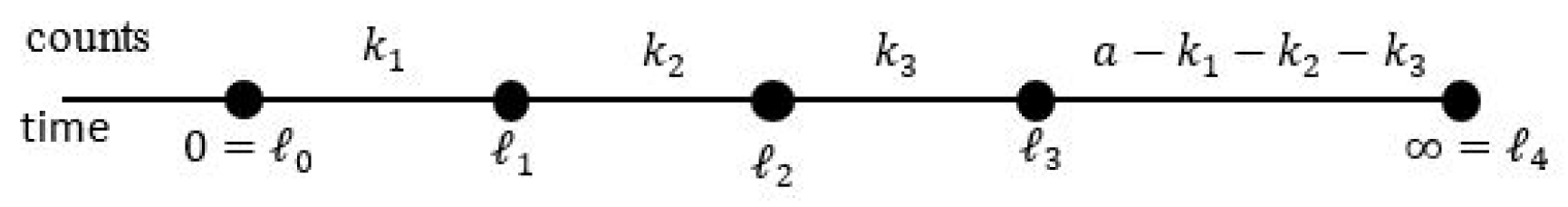
In this section we state the mathematical foundation of our approach, see Table 1. We start with a subsection in which we state the notation that we use in this paper, and then continue with two subsections on the distribution of bug detection times that we need to derive the likelihood function. In a subsequent subsection we present a Bayesian approach to our feature-specific model.

2.1. Notation

Capital letters are used for random quantities, small letters for constants, or model parameters. We follow the setup as is explained in the GQS setting, see Table 1. A software tool has a bugs, which are detected at time T i after testing starts at time 0. As usual in industrial practice, these times are not observed or recorded directly. Instead, we only observe number of bugs detected in time intervals. This kind of data is known as grouped data, which is a form of interval censoring. For now, we do not distinguish between different features.
Throughout, we assume that the T i ’s are independent and identically distributed. Throughout, we assume that the T i ’s are independent and identically distributed (further denoted by i.i.d). Identically distributed implies that are defects are equally hard to find, even though works has been done to relax this. We realize the impact of this assumption. The Jelinski–Moranda [14] model additionally assumes the T i ’s are exponentially distributed with rate b, so all T i Exp ( b ) . We explicitly mention when we make the same assumption. In our setting, we assume that we only observe counts N i in contiguous time periods with start and end points 0 = 0 < 1 < 2 < , i.e., N i = j = 1 a 1 ( i 1 < T j i ) .

2.2. Multinomial Distribution of Bug Counts

As the times T j are independent, the joint probability distribution of increments in numbers of bugs over a finite set of observation intervals is given by a multinomial distribution. Consider the event E i j that j 1 T i j . Then for each bug i, exactly one of the mutually exclusive events E i j occurs. Considering that bug i is found at time T i , the probability that event E i j occurs is given by F ( j ) F ( j 1 ) , which is the same for each bug i. In view of the independence, we have the settings of a multinomial distribution [22]. We give the full probability distribution in a few different ways that are used later on. Let m L and let T denote a random variable with the same distribution as the T i ’s. Then we have
P ( N 1 = k 1 , , N m = k m ) = a k 1 , , k m i = 1 m F ( i ) F ( i 1 ) k i 1 F ( m ) a ( k 1 + + k m ) = a k 1 , , k m i = 1 m P ( i 1 < T i ) k i P ( m < T ) a ( k 1 + k m ) = a k 1 , , k m i = 1 m + 1 P ( i 1 < T i ) k i
where in the last step we set m + 1 = , F ( m + 1 ) = 1 , and k m + 1 = a ( k 1 + + k m ) for notational convenience (see Figure 2). The expression before the product is the multinomial coefficient, a generalization of the binomial coefficient.

2.3. Conditioning on History

In what follows, we study the joint probability distribution conditional on the history up to some point m . We will need this to combine the different sprint. It turns out it is sufficient to summarize the entire history prior to m by the total bug count at this time point. If we assume exponentially distributed bug detection times T i , it appears that a restarting property holds. At time point m , a certain number of bugs remains in the system. The conditional joint probability distribution is again multinomial and corresponds to the above result after proper bookkeeping: shifting the time axis so that m corresponds to the new 0, and work with the remaining number of bugs at this time point. This is summarized in the following two results.
In the notation above, suppose the bug detection times T i are i.i.d. with cumulative probability function F. Writing the definition of conditional probability and cancelling common terms in the numerator and denominator, we obtain that
P ( N m + s = k m + s , , N m + 1 = k m + 1 N m = k m , , N 1 = k 1 ) = P ( N m + s = k m + s , , N m + 1 = k m + 1 C m = k 1 + + k m ) .
Moreover, substitution of our expression for the joint distribution of bug counts, it is easy to see that this conditional probability is equal to
a k 1 k m k m + 1 , , k m + s i = 1 s + 1 F ( m + i ) F ( m + i 1 ) k m + i 1 F ( m ) a ( k 1 + k m )
where we set m + s + 1 = , F ( m + s + 1 ) = 1 , and k m + s + 1 = a ( k 1 + + k m + s ) for notational convenience.
We will also need the specific form of the likelihood under the additional assumption that T j follows an exponential distribution. Although we only use it for one sprint forward into time, a more general result holds for s sprints into the future given in the following result. In the notation above, suppose the i.i.d. bug detection times T i follow an exponential distribution as in the Jelinski–Moranda setting. We see that the joint probability distribution condition on history until time m is the same as the multinomial distribution with quantities as if we start over.
P ( N m + s = k m + s , , N m + 1 = k m + 1 N m = k m , , N 1 = k 1 ) = a k 1 k m k m + 1 , , k m + s i = 1 s + 1 P ( m + i 1 T m + i T > m ) k m + i )
where as before we set m + s + 1 = , F ( m + s + 1 ) = 1 , and k m + s + 1 = a ( k 1 + + k m + s ) for notional convenience. The conditional probabilities are given by:
P ( m + i 1 T m + i T > m ) = e b ( m + i 1 m ) e b ( m + i m )
which are the same as the unconditional probabilities if we would shift the time axis so that m would lie at zero. The history until m only enters the formulas via the sum of counts k 1 + + k m .
For the implementation later on, we only use the special case s = 1 , which gives the following result. P ( N m + 1 = k m + 1 N m = k m , , N 1 = k 1 ) is given by a formula as in a binomial distribution, where the conditioning on history can be summarized by C m = k 1 + + k m . The probability density is equal to:
P ( N m + 1 = k m + 1 N m = k m , , N 1 = k 1 ) = P ( N m + 1 = k m + 1 C m = k 1 + + k m ) = a k 1 k m k m + 1 1 e b ( m + 1 m ) k m + 1 · = e b ( m + 1 m ) 1 a ( k 1 + + k m + 1 )
We now set out to show that these binomial densities can be combined in a product over the sprints to form the full joint probability, which is used in the implementation to get an expression for the likelihood. In the setting above, assuming exponentially distributed bug detection times, the joint probability mass function of the counts ( N 1 , , N m ) is given by the product over the sprints of the densities of the conditional binomial expressions given above:
P ( N 1 = k 1 , , N m = k m ) = i = 1 m P ( N i = k i C i 1 = k 1 + k i 1 )
This can be seen as follows. The event ( N m = k m , , N 1 = k 1 ) can be rewritten into its cumulative count version ( C m = c m , , C 1 = c 1 ) with c i = c i 1 + k i and c 1 = k 1 . We use the chain rule for probabilities, e.g., for m = 3 we have P ( C 3 = c 3 , C 2 = c 2 , C 1 = c 1 ) = P ( C 3 = 3 C 2 = c 2 , C 1 = c 1 ) · P ( C 2 = c 2 C 1 = c 1 ) · P ( C 1 = c 1 ) . Here, the history-by-total-count result allows us to simplify the event on which we condition to only the most recent cumulative count: P ( C 3 = c 3 C 2 = c 2 , C 1 = c 1 ) = P ( C 3 = c 3 C 2 = c 2 ) .

2.4. Extension to Multiple Features

As explained in the introduction, the situation of interest consists not just of one fixed software implementation but of a growing software implementation, where bugs are labeled to which feature they belong. A feature here means a certain functionality in the software. For example, open or close a window in the user interface. Or, in the case of a connected lighting application, dimming the light levels. A new feature in an agile environment may be added every so-called sprint. Here, a sprint means 2–3 weeks of software development. We assume that exactly one feature is added in every time interval between i and i + 1 , although this assumption is not essential and is merely done to keep notation simple. Ahead, we sketch how the general case of features being finished at arbitrary times can be incorporated. Thus we have features f = 0 , , L 1 where each feature f is finished at time point f and subject to testing from that point in time onward. We assume that the test intensity for each feature is constant over time, even though new features might be added that could take up testing capacity of the older features. Each feature has a f bugs in total which is considered fixed for now. The a f bugs of this feature are found at times T f , 1 , , T f , a f that are shifted exponential distributions that start at time point f , so that T f , i f is exponentially distribution with parameter b f . The CDF is F T f , i ( t ) = exp ( b ( t f ) ) for t f and 0 for t < f . The time points i are common to all features and do not get an additional index for f. This way, we arrive at a description of bugs labeled for different features. Following the above, it is stated for unshifted exponential distributions, although one can imagine a version for shifted (replacing e b i with e b ( i f ) ) and keeping proper track of what happens before time f (e.g., by defining 0 0 = 1 in the product). Instead of generalizing these results, we take a different path which is also closer to the software interpretation, by simply shifting the time axis. Note that we assumed that feature f is finished at time point l f . For the case where new features do not coincide exactly with sprints, say that feature f is finished at time l t ( f ) , where t is increasing. The shifts are defined accordingly, l m = l m l t ( f ) and N ( f + 1 ) is replaced by N ( t ( f ) + 1 ) . We assume that bugs can be ascribed to a single feature in this model, and that detection happens independently between the features, even though in some respects one would expect connections between different features, or even bugs on the interface between two features. These are not explicitly covered in the current model.
To set up notation for shifting the time axis, we fix the feature f and drop it from notation of the new symbols, and add an apostrophe to each symbol to indicate it is the shifted time or event. Let m f . Define T i = T f , i f , and m = m f , which describes the shifted time axis. We also need to translate the history event. Define N i = N i + f , the number of bugs found in interval [ i + f 1 , i + f ] , so that N 1 corresponds to the first interval on our shifted time axis, [ f , f + 1 ] . Consider the event ( N 1 = k 1 , N m = k m ) . Rewriting from relative to absolute time gives ( N f + 1 = k f + 1 , N f + m = k f + m ) with k i + f = k i to match the indexing. The only possible realizations for N 1 , , N f 1 are 0 due to the shifted exponential distribution, so that the event corresponds to ( N 1 = 0 , , N f = 0 , N f + 1 = k f + 1 , N f + m = k f + m ) and has equal probability. We use the conditional binomial restarting result from above and note that the shifted version of the problem satisfies the condition.
P ( N m + 1 = k m + 1 N m = k m , , N 1 = k 1 ) = a k 1 k m k m + 1 1 e b ( m + 1 m ) k m + 1 · = e b ( m + 1 m ) 1 a ( k 1 + + k m + 1 )
This results in an expression for the probability density function of the number of bugs found for feature f, conditional on what happened just before. These can then be combined to form the full probability density function on the shifted time axis, which subsequently is the same event as the one with leading 0 counts on the unshifted time axis. We re-introduce the feature index f and note that the above is equal to P ( N f , m + 1 = k f , m + 1 C f m = k f 1 + + k f m ) where the symbols N f , i and C f , i are the feature-specific counterparts of N i and C i . We assume that all bug discovery times T f , i are independent, which implies that the random variables N f , i and N g , j are independent as well for any i , j and features f g . We summarize this as follows. In generalizing the setup to multiple features f as described above, at time point m , features 0 , , m have been added to the software and have observed counts up to that time point. The probability density of the counts up to m is found by taking a product over the features f of the feature-specific probabilities. These are given by a product of binomial distributions of time-shifted versions. Viewing the density function as the likelihood function, the parameters are the a f and b f for f = 0 , , m .

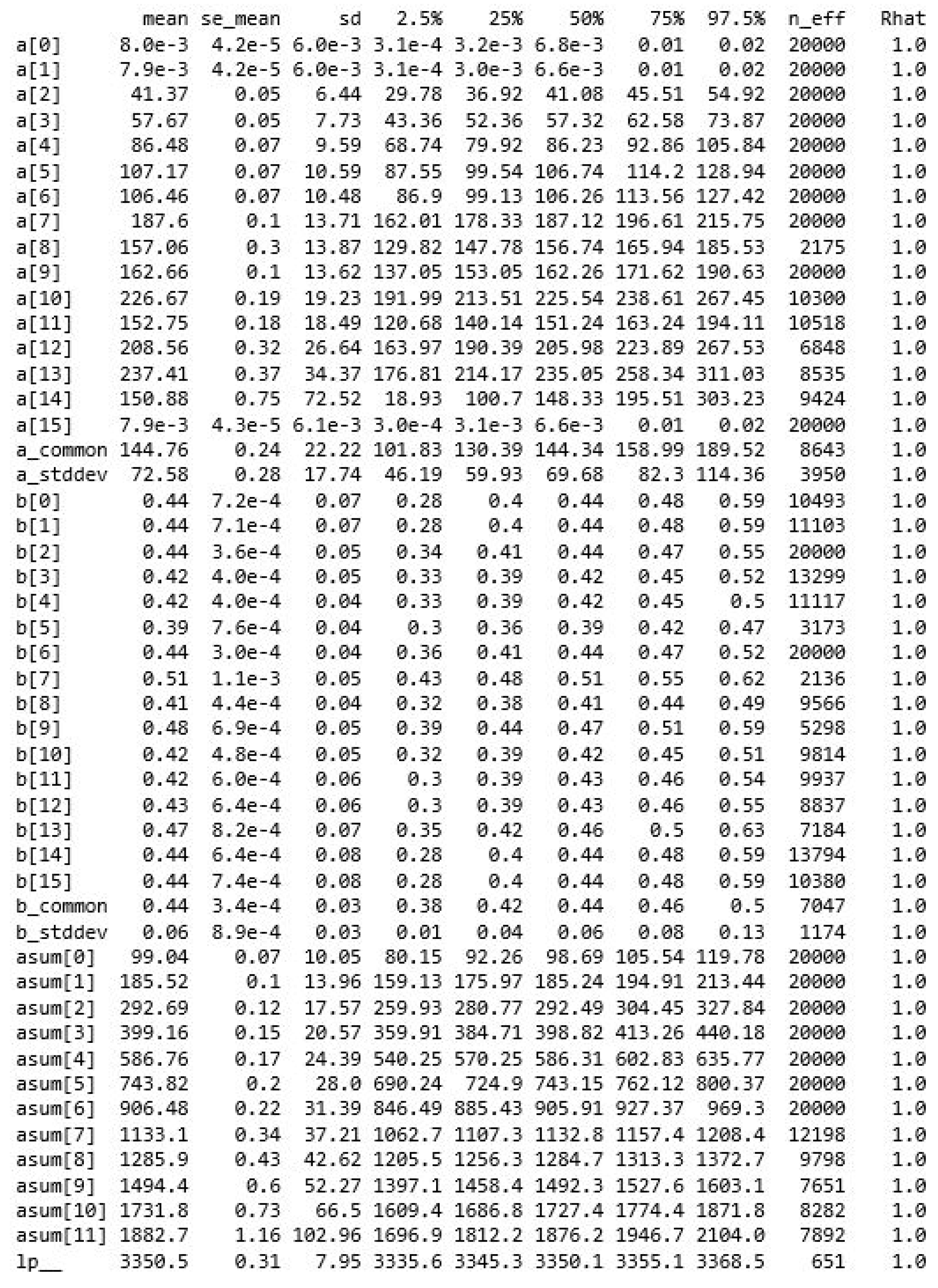
2.5. Bayesian Estimation

It is well-known that the maximum likelihood estimator for a has a positive probability to be equal to infinity (see e.g., [23,24]). We use a Bayesian setup [25,26,27,28] to avoid this problem and also because it allows us to combine the bugs originating from different features. We implemented our Bayesian approach in the Stan modeling framework [29] to estimate the software reliability model for multiple features. We do not employ strong priors although that would be possible, e.g., expressing a prior belief of the degree to which added features are similar to each other in total number of bugs a f or the speed at which bugs are found, b f . For a feature f, given values for ( a f , b f ) , the setup from above is in essence a Jelinski–Moranda model. The values ( a f , b f ) are considered random, unknown parameters, having the same role as random effects in a (non)linear mixed effects model following some distribution. In a Bayesian context, the a f , b f can be considered priors with associated hyperpriors. In our setup, a f and b f are modeled as independent truncated normal distributions, where the truncation are at 0 to ensure positive a f and b f . Both distributions have a mean and standard deviation parameter, although they are not equal to the expected value and standard deviation due to the truncation. Their posterior distributions give some insight to which extent features are different in size and complexity (in terms of speed of finding bugs). The reading of input data, pre-processing the data, fitting the Stan model, and inspecting convergence and results are done using Python. The Stan website (mc-stan.org) states “Stan is a state-of-the-art platform for statistical modeling and high-performance statistical computation”. The website offers an extensive amount of documentation and examples. The Stan language requires specification of a model in terms of different concepts which are briefly described below. The model is applied in the situation that we have observed a number of sprints with counts to which we fit the data. The key Stan model components are as follow:
  • input data: the N f , i , C f , i , upper bounds for the indices f and i, and time point at which a feature starts;
  • parameters: total bugs remaining, R f : = a f C f , m , with a lower bound of 0; the b f ; the hyperpriors for the truncated normal distributions of a f and b f ;
  • transformed parameters: a f is considered a transformed parameter, calculated from a combination of data and a model parameter, R f + C m , f ;
  • model: distributions for a f and b f , hyperpriors for these, and a specification of log likelihood contributions by a double for-loop over features and over sprints, where the feature starting sprints are used.
In this setup, there is a notable construction of R f that has no direct correspondence to the mathematical setup. The reason is that Stan needs explicit, fixed bounds for the parameters in order for the numerical engine to simulate the posterior density, and the data-dependent bound a f C f , m is enforced by R f 0 . It is still possible to set priors on a f rather than the actual model parameter R f , via a line of code inside a loop over the features that corresponds to R f + C f , m N ( μ , σ ) where the truncation a f is specified in the definition of a f . For ease of use, the statistics is programmed in Python and Stan, which handles the estimation and handling of Bayesian models in a user-friendly tool.

3. Use Cases

In order to explore the abilities of the coding, two cases are used. The first one concerns publicly available software test data [30] and the second one is a real case from the lighting industry [4].

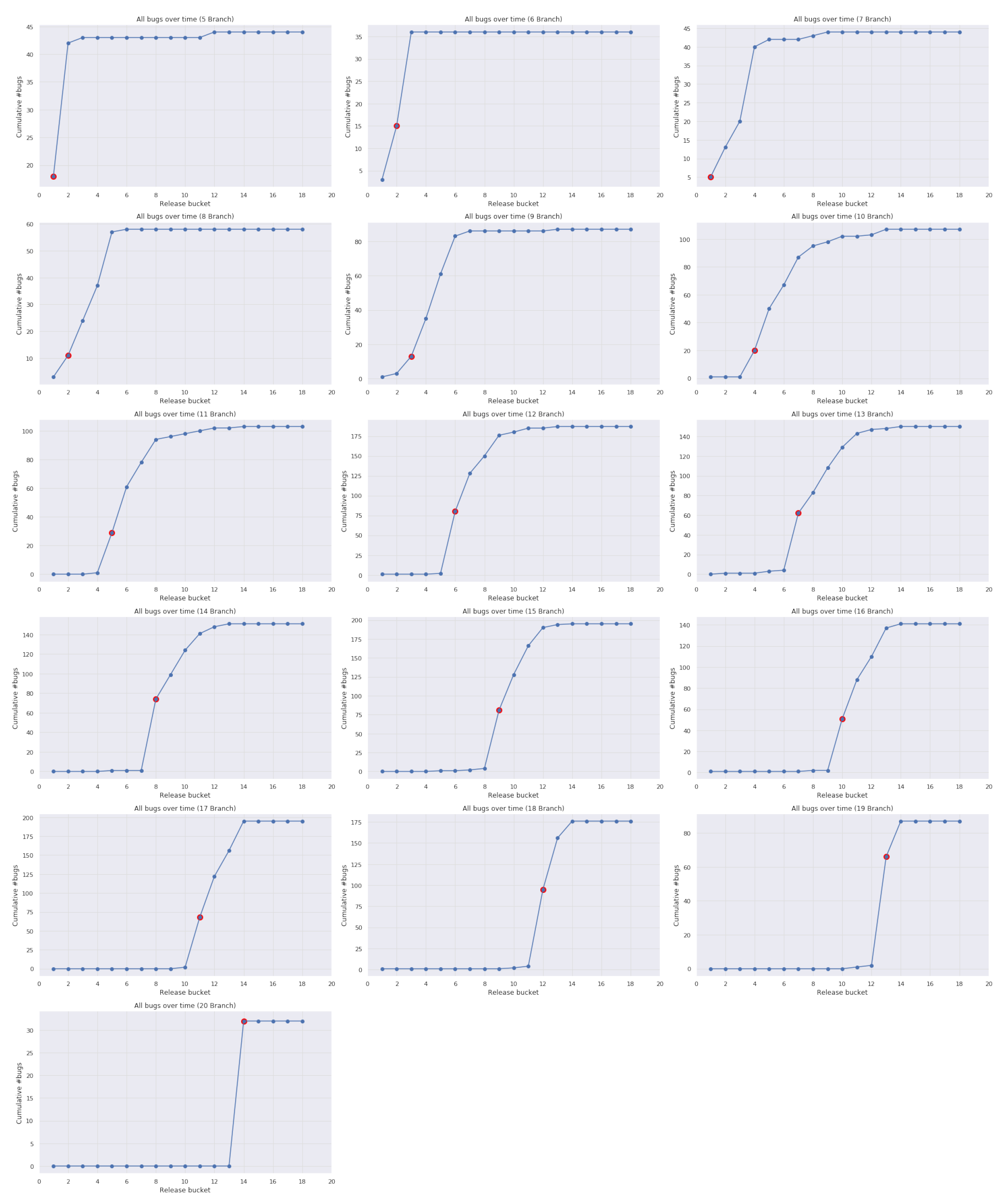
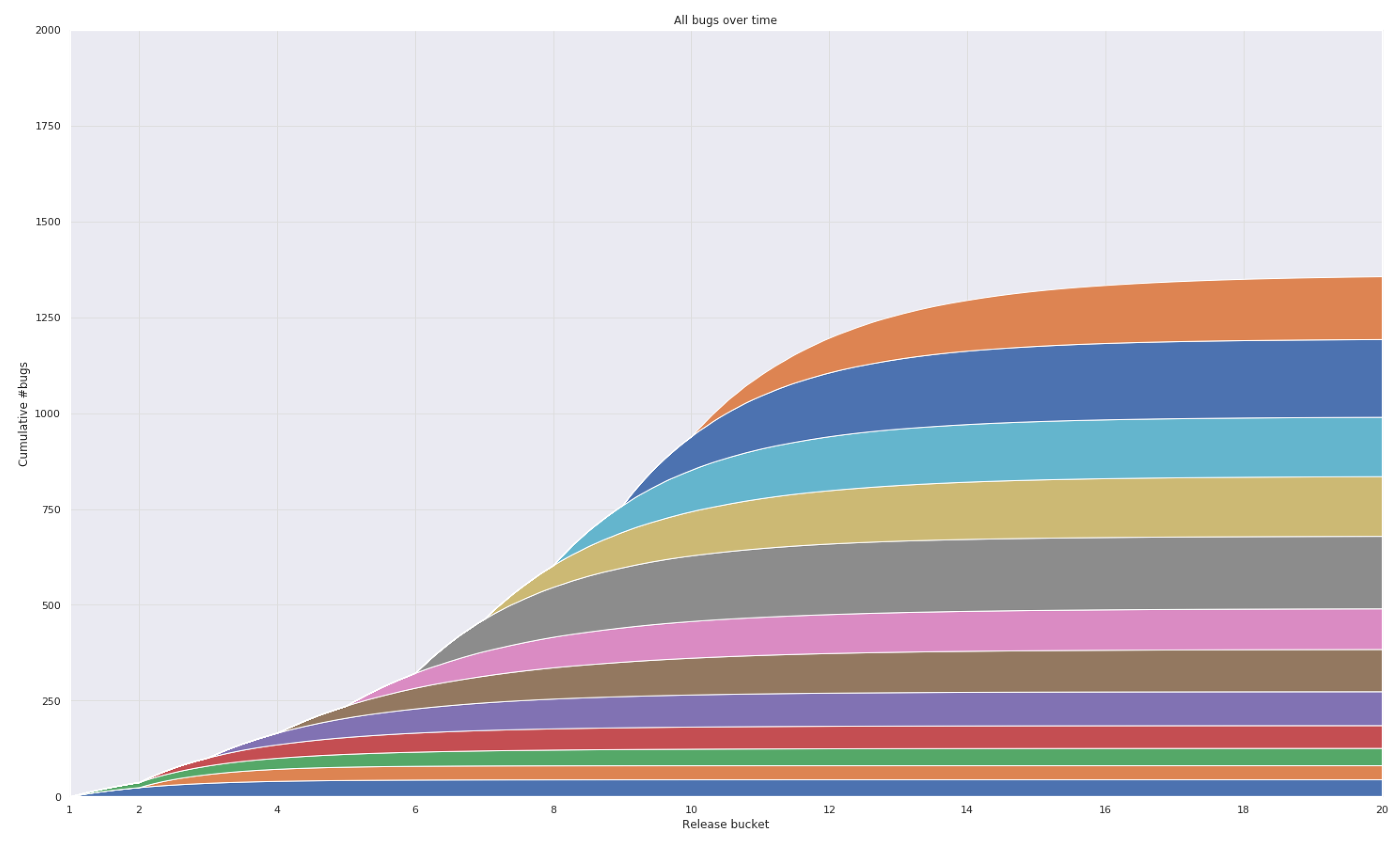
3.1. Case 1: Firefox Data

We used the Mozilla and Eclipse Defect Tracking Data set: a data set with over 200 , 000 reported bugs extracted from the Eclipse and Mozilla projects ( 47 , 000 and 168 , 000 reported bugs, respectively) [30]. Typically, in software development, features are developed in branches that are later merged with the main branch (call it a main feature). We assume here the one-to-one correspondence between branch and feature. In the case presented, there are 15 main features (or functions). Besides providing a single snapshot of a bug report, this data set also includes all the incremental modifications as performed during the lifetime of the bug report. This data set is bundled as a set of XML files. We extracted reported bugs for a number of 15 branches over a time period staring at January 2003 until May 2013. The total number of reported bugs in this time period is 1793. Figure 3 depicts the fitted response for all individual branches (or features). Figure 4 depicts the same information in a single plot. The priors have been chosen so that they are uninformative for our dataset. For instance, b is the rate of bug detection. The variable std_rate is the standard deviation of the rates between features. One divided by the rate is the time it takes before 1 exp ( 1 ) = 0.63 of all bugs are found. The standard deviation is taken as the positive half of a normal distribution with m e a n = 0 and s t d e v = 1 . This is fairly large compared to our average rate. In the output the a i ’s are the total amount of software defects, or bugs for branch/feature nr 3. The b i ’s are bug_finding_rate[3]. The a i ’s and b i ’s are both normally distributed (between features) with means, standard deviation avg_bugs, std_bugs, and avg_rate, std_rate respectively. The mean and a high percentile are interesting here—the 97.5 percentile column indicates that given the current data we believe that the number of additional bugs over so many time periods is with 97.5 percent chance at most the indicated value. The se_mean is the Monte Carlo uncertainty (the fact that in model estimation we used only limited computer time—with more computer time we can get this number down). The 2.5 and 97.5 percentiles indicate the posterior distribution of the given parameter. The n_eff gives the effective sample size from the simulation. Rhat is an indication of quality of the estimation procedure and should be close to 1.0 . The estimation may give a warning in case of problems, e.g., if the data severely deviates with the model assumptions in.
See Figure 5 for diagnostic plots of the fit. Table 2 lists the average and standard deviation of predicted remaining bugs in the software. The low numbers are due to the fact that the model prediction for the number of remaining bugs is formally for the case if no further development (other than bug fixing) takes place. As in reality, new features kept being added for this case and the number of bugs increased over time.

3.2. Case 2: Industrial Data

As a real application case, we took a connected lighting product that enables you to harness the Internet of Things to transform your building and save up to 80 percent on energy. LED luminaries with integrated sensors collect anonymous data on lighting performance and how workers use the workplace. This enables you to optimize the lighting, energy uses, cleaning, and space usage to improve efficiency, reducing energy usage, and cost. Workers can use software apps on their smartphones to book meeting rooms, navigate within the office and personalize the environment around their workstation further improving productivity and employee engagement. This smart lighting system with open API integrates seamlessly with the IT system and enables a variety of software applications to create a more intelligent work environment for both building operations managers and employees. In literature, the use of software development schemes and repositories are well described [32,33,34]. It is demonstrated that detailed problem handling reports will extend the space and quality of statistical analysis for software [34]. It is without doubts that detailed reports will provide significant improvement of software development processes as well as better reliability predictions [32]. In this case, the bug reports may come from different sources (implemented regression tests and tests by the team). Only bugs of sufficient severity are considered in the use case. To handle the various sources we simply took the aggregate counts per sprint as input, assuming that the total number of tests in a sprint was comparable, we get a discrete time axis that was reasonably close to both test effort and calendar time. Ticket data were fed into the code, where we distinguished tickets with severity levels S (high) and A (low). We used JIRA [35] output of bug data for 40 sprints in the period 2017 until 2019. Pick-and-mix was used for ticket severity allocation. In a cadence of two weeks, these tickets either had the allocation open or closed. Open means the issues were being solved, closed means it was solved. Recurring tickets were treated as a new open ticket which can be closed as soon as it is known to be recurrent. Ticket severity is denoted as S, A, B, C, or D. S are issues seen as a blocker that need immediate attention. A is seen as critical, B as major C and D as minor severity levels. In the case presented, we have only analyzed the closed tickets.
Figure 6 depicts the full flowchart of the process: from tickets to dashboard values. Actual sprint dates have an equal length for each sprint of two weeks. The total number of bugs was 270. The outcome was produced automatically and shown in Table 3 and Figure 7. The results indicate the predicted remaining number of tickets in the weeks (or sprints) to come, if no new features would be added and only testing is performed. In the figure and table, one clearly notices the maturity of the software.

4. Discussion

Software failures differ significantly from hardware failures. They are not caused by faulty components or wear-out due to e.g., physical environment stresses such as temperature, moisture, and vibration, software failures are caused by latent software defects. These defects were introduced in the software when it was created. However, these defects were not detected and/or removed prior to being released to the customer. In order to prevent these defects being noticed by the customer, a higher level of software reliability has to be achieved. This means to reduce the likelihood that latent defects are present in released software. Unfortunately, even with the most highly skilled software engineers following the best industry practices, the introduction of software defects is inevitable. This is due to the ever-increasing inherent complexities of the software functionality and its execution environment. Here, software reliability engineering may be helpful, a field that relates to testing and modeling of software functionality in a given environment of a particular amount of time. There is currently no method available that can guarantee a totally reliable software. In order to achieve the best possible software, a set of statistical modeling techniques are required that:
  • can assess or predict the to-be-achieved reliability;
  • based on the observations of software failures during testing and/or operational use.
In order to achieve these two requirements, many software reliability models have been proposed. It was shown that, once these models reach a certain level of convergence, it can enable the developer to release the software and stop software testing accordingly. Criteria to determine the optimal testing time include the number of remaining errors, failure rate, reliability requirements, or total system cost. Typical questions that need to be addressed are:
  • how many errors are still left in the software?
  • what is the probability of having no failures in a given time period?
  • what is the expected time until the next software failure will occur?
  • what is the expected number of total software failures in a given time period?
Certainly, the question of “how many errors are left” is something completely different from “what is the expected number of errors in a given time period”. One cannot estimate the first directly, but you can estimate the second. In our approach, we are content with “expected number of errors that a long testing period would yield”.
In this paper, we presented an approach to predict software reliability for agile testing environments. The new approach divers from the many others in the sense that it combines features with tickets using Bayesian statistics. By doing that, a more reliable number of predicted tickets (read: software bugs) can be obtained. The advantage of this overall model by applying the JM model per feature is (1) to be able to get prediction intervals for the total number of remaining bugs across all features combined, and (2) “borrowing strength”—we saw in our test cases that a f and b f are relatively similar so that for a new feature even after few bugs one knows more than when you analyze features separately, which is the advantage of the overall combined analysis. The developed system software reliability approach was applied to two use cases, Mozilla and Lighting, to demonstrate how software reliability models can be used to improve the quality metrics. The new approach was made into a tool, programmed in Python. The outcome of the predictions can be used in the Quality dashboard maturity grid to enable a better judgment of whether to release the software. The strength of the software reliability approach is to be proven by more data and comparison with field return data. The outcome is satisfactory as a more reliable number of remaining tickets was calculated. As prominent advantage we note that divergence of the proposed fitting procedure is not an issue anymore in the new approach. Following is recommended for the future developments of the presented approach:
  • gather more data from the software development teams;
  • connect to the field quality community to gather field data of software tickets;
  • using the field data determine the validity of the approach;
  • make software reliability calculation part of the development process;
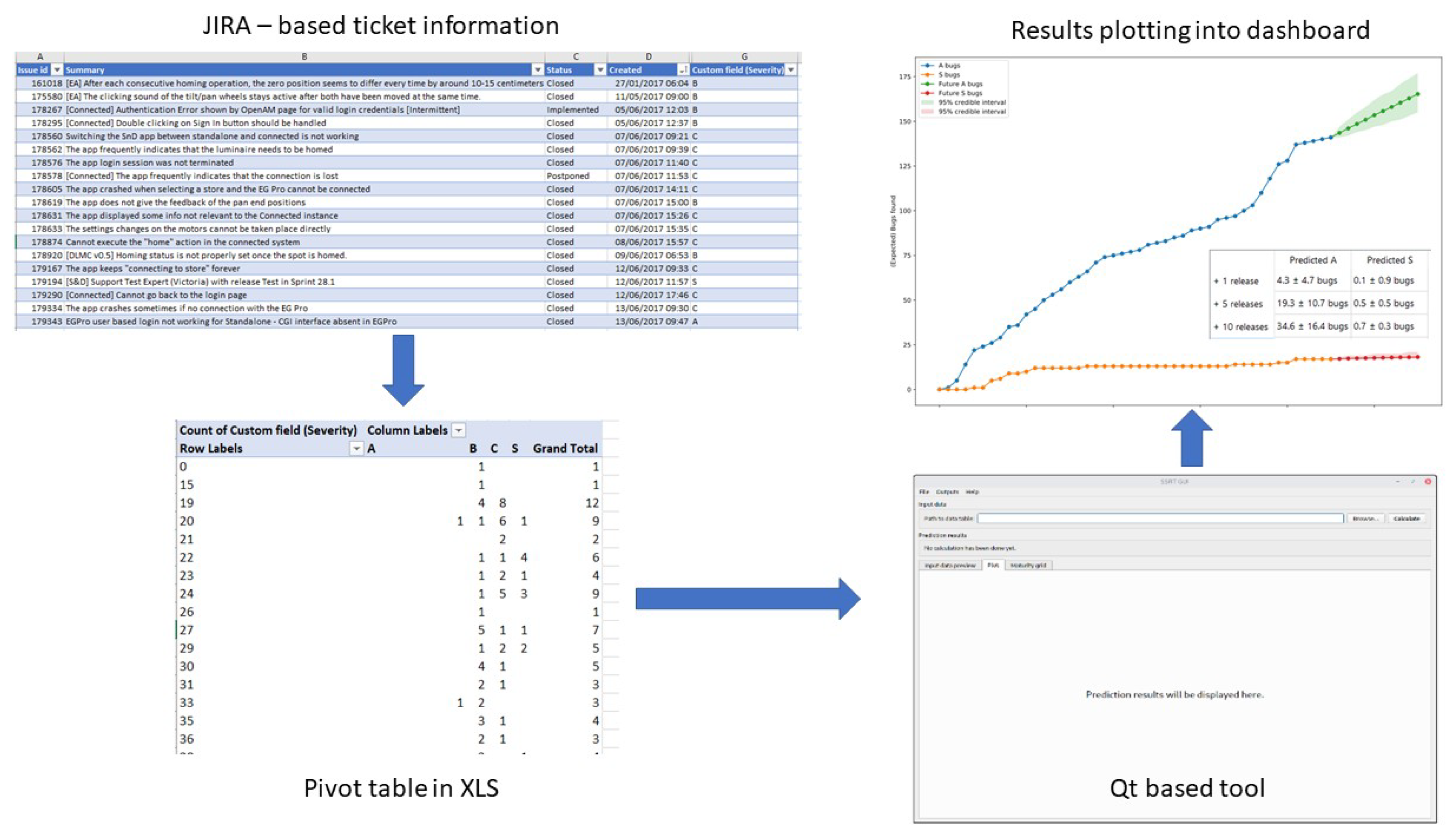
  • automate the Python code such that ticket-feature data can be imported on-the-fly;
  • include machine learning techniques and online failure prediction methods, which can be used to predict if a failure will happen 5 min from now [36];
  • investigate the use of other SRGM models, including multistage ones, or those that can distinguish development and maintenance software defects [17,18];
  • not focus on a specific software reliability model but rather assess forecast accuracy and then improve forecasts as was demonstrated by Zhao et al. [37];
  • classify the expected shape of defect inflow prior to the prediction [18].

Author Contributions

W.D.v.D.: methodology, writing—original draft preparation; J.W.B.: conceptualization, project administration, and investigation; M.T.: conceptualization, writing—review and editing, software, and investigation; A.D.B.: writing—review and editing, supervision, and conceptualization. All authors have read and agreed to the published version of the manuscript.

Funding

This research received no external funding.

Conflicts of Interest

The authors declare no conflict of interest.

References

  1. Van Driel, W.; Fan, X. Solid State Lighting Reliability: Components to Systems; Springer: New York, NY, USA, 2012. [Google Scholar] [CrossRef]
  2. Van Driel, W.; Fan, X.; Zhang, G. Solid State Lighting Reliability: Components to Systems Part II; Springer: New York, NY, USA, 2016. [Google Scholar] [CrossRef]
  3. Papp, Z.; Exarchakos, G. (Eds.) Runtime Reconfiguration in Networked Embedded Systems—Design and Testing Practice; Springer: Singapore, 2016. [Google Scholar] [CrossRef]
  4. Van Driel, W.; Schuld, M.; Wijgers, R.; Kooten, W. Software reliability and its interaction with hardware reliability. In Proceedings of the 15th International Conference on Thermal, Mechanical and Multi-Physics Simulation and Experiments in Microelectronics and Microsystems (EuroSimE), Ghent, Belgium, 7–9 April 2014. [Google Scholar]
  5. Abdel-Ghaly, A.A.; Chan, P.Y.; Littlewood, B. Evaluation of competing software reliability predictions. IEEE Trans. Softw. Eng. 1986, SE-12, 950–967. [Google Scholar] [CrossRef]
  6. Bendell, A.; Mellor, P. (Eds.) Software Reliability: State of the Art Report; Pergamon Infotech Limited: Maidenhead, UK, 1986. [Google Scholar]
  7. Lyu, M. (Ed.) Handbook of Software Reliability Engineering; McGraw-Hill and IEEE Computer Society: New York, NY, USA, 1996. [Google Scholar]
  8. Pham, H. (Ed.) Software Reliability and Testing; IEEE Computer Society Press: Los Alamitos, CA, USA, 1995. [Google Scholar]
  9. Xie, M. Software reliability models—Past, present and future. In Recent Advances in Reliability Theory (Bordeaux, 2000); Stat. Ind. Technol.; Birkhäuser Boston: Boston, MA, USA, 2000; pp. 325–340. [Google Scholar]
  10. Bishop, P.; Povyakalo, A. Deriving a frequentist conservative confidence bound for probability of failure per demand for systems with different operational and test profiles. Reliab. Eng. Syst. Safety 2017, 158, 246–253. [Google Scholar] [CrossRef]
  11. Adams, E. Optimizing preventive service of software products. IBM J. Res. Dev. 1984, 28, 2–14. [Google Scholar] [CrossRef]
  12. Miller, D. Exponential order statistic models of software reliability growth. IEEE Trans. Softw. Eng. 1986, SE-12, 12–24. [Google Scholar] [CrossRef]
  13. Joe, H. Statistical Inference for General-Order-Statistics and Nonhomogeneous-Poisson-Process Software Reliability Models. IEEE Trans. Software Eng. 1989, 15, 1485–1490. [Google Scholar] [CrossRef]
  14. Jelinski, Z.; Moranda, P. Software Reliability Research. In Statistical Computer Performance Evaluation; Freiberger, W., Ed.; Academic Press: Cambridge, MA, USA, 1972; pp. 465–497. [Google Scholar]
  15. Xie, M.; Hong, G. Software reliability modeling, estimation and analysis. In Advances in Reliability; North-Holland: Amsterdam, The Netherlands, 2001; Volume 20, pp. 707–731. [Google Scholar]
  16. Almering, V.; Van Genuchten, M.; Cloudt, G.; Sonnemans, P. Using Software Reliability Growth Models in Practice. Softw. IEEE 2007, 24, 82–88. [Google Scholar] [CrossRef] [Green Version]
  17. Pham, H. (Ed.) System Software Reliability; Springer: London, UK, 2000. [Google Scholar] [CrossRef]
  18. Rana, R.; Staron, M.; Berger, C.; Hansson, J.; Nilsson, M.; Törner, F.; Meding, W.; Höglund, C. Selecting software reliability growth models and improving their predictive accuracy using historical projects data. J. Syst. Softw. 2014, 98, 59–78. [Google Scholar] [CrossRef]
  19. Xie, M.; Hong, G.; Wohlin, C. Modeling and analysis of software system reliability. In Case Studies in Reliability and Maintenance; Blischke, W., Murthy, D., Eds.; Wiley: New York, NY, USA, 2003; Chapter 10; pp. 233–249. [Google Scholar]
  20. Dalal, S.R.; Mallows, C.L. When should one stop testing software? J. Amer. Statist. Assoc. 1988, 83, 872–879. [Google Scholar] [CrossRef]
  21. Zacks, S. Sequential procedures in software reliability testing. In Recent Advances in Life-Testing and Reliability; CRC: Boca Raton, FL, USA, 1995; pp. 107–126. [Google Scholar]
  22. Johnson, N.; Kemp, A.; Kotz, S. Univariate Discrete Distributions; Wiley Series in Probability and Statistics; Wiley: New York, NY, USA, 2005. [Google Scholar]
  23. Blumenthal, S.; Dahiya, R. Estimation of sample size with grouped data. J. Stat. Plan. Inference 1995, 44, 95–115. [Google Scholar] [CrossRef]
  24. Littlewood, B.; Verrall, J.L. Likelihood function of a debugging model for computer software reliability. IEEE Trans. Rel. 1981, 30, 145–148. [Google Scholar] [CrossRef]
  25. Bai, C.G. Bayesian network based software reliability prediction with an operational profile. J. Syst. Softw. 2005, 77, 103–112. [Google Scholar] [CrossRef]
  26. Basu, S.; Ebrahimi, N. Bayesian software reliability models based on martingale processes. Technometrics 2003, 45, 150–158. [Google Scholar] [CrossRef]
  27. Littlewood, B.; Sofer, A. A Bayesian modification to the Jelinski-Moranda software reliability growth model. Softw. Eng. J. 1987, 2, 30–41. [Google Scholar] [CrossRef] [Green Version]
  28. Littlewood, B. Stochastic reliability-growth: A model for fault-removal in computer-programs and hardware-designs. IEEE Trans. Reliab. 1981, 30, 313–320. [Google Scholar] [CrossRef]
  29. Team, T.S.D. Stan Python Code. 2018. Available online: https://mc-stan.org/ (accessed on 15 November 2018).
  30. Lamkanfi, A.; Perez, J.; Demeyer, S. The Eclipse and Mozilla Defect Tracking Dataset: a Genuine Dataset for Mining Bug Information. In Proceedings of the MSR ’13 10th Working Conference on Mining Software Repositories, San Francisco, CA, USA, 18–19 May 2013. [Google Scholar]
  31. Depaoli, S.; van de Schoot, R. Improving Transparency and Replication in Bayesian Statistics: The WAMBS-Checklist. Psychol. Methods 2017, 22, 240–261. [Google Scholar] [CrossRef] [PubMed]
  32. Janczarek, P.; Sosnowski, J. Investigating software testing and maintenance reports: case study. Inf. Softw. Technol. 2015, 58, 272–288. [Google Scholar] [CrossRef]
  33. Rathore, S.; Kumar, S. An empirical study of some software fault prediction techniques for the number of faults prediction. Soft Comput. 2017, 21, 7417–7434. [Google Scholar] [CrossRef]
  34. Sosnowski, J.; Dobrzyński, B.; Janczarek, P. Analysing problem handling schemes in software projects. Inf. Softw. Technol. 2017, 91, 56–71. [Google Scholar] [CrossRef]
  35. Atlassian. JIRA Software Description. 2020. Available online: https://www.atlassian.com/software/jira (accessed on 12 May 2020).
  36. Salfner, F.; Lenk, M.; Malek, M. A survey of online failure prediction methods. ACM Comput. Surv. 2010, 42, 12–24. [Google Scholar] [CrossRef]
  37. Zhao, X.; Robu, V.; Flynn, D.; Salako, K.; Strigini, L. Assessing the Safety and Reliability of Autonomous Vehicles from Road Testing. In Proceedings of the 30th International Symposium on Software Reliability Engineering (ISSRE), Berlin, Germany, 28 October–1 November 2019. [Google Scholar]
Figure 1. The growing population with increased urbanization results in the need to focus on energy efficiency and sustainability, thereby increasing digitization and rapidly evolving technologies containing software.
Mathematics 08 00791 g001
Figure 2. Representation of the time axis.
Mathematics 08 00791 g002
Figure 3. Fit of individual branches or features in the data set, the red dot is the first data point estimated. Here, each branch is considered as a feature which are plotted separately.
Mathematics 08 00791 g003
Figure 4. Fitted bugs per branch. Here, each branch is considered as a feature which are visualized with different colors in the fit.
Mathematics 08 00791 g004
Figure 5. Inference and diagnostics for the software reliability prediction model. Diagnostics are explained in the text and follow [31]. Here, a is total number of bugs, b is the bug finding rate and asum relates to the number of future bugs.
Mathematics 08 00791 g005
Figure 6. Flowchart for automatic generation of software reliability predictions. Details are explained in the text.
Mathematics 08 00791 g006
Figure 7. Fit of tickets with S-bugs in the lighting case. Horizontal axes is the time in agile sprints, in this particular case of two weeks, vertical axes shows the total number of bugs with annotation S (high level of severity).
Mathematics 08 00791 g007
Table 1. Symbols used in the Jelinski–Moranda model for grouped data.
SymbolRandomDomainMeaning
aNo N Initial number of bugs
bNo R + Rate of bug detection
T i Yes R + Time at which bug i is found
LNo N Number of intervals
i No R + End time of interval i
N i Yes N Number of bugs found in the time interval [ i 1 , i ]
C i Yes N Cumulative number of bugs detected until i , C i = N 1 + + N i
Table 2. Predicted number of remaining bugs.
BranchAverageStdev
+14.53.5
+512.04.0
+1015.23.8
Table 3. Predicted number of remaining bugs in the lighting case. Sprints here refers to two weeks development of the software.
SprintAverageStdev
+10.20.8
+50.82.2
+101.52.6

