A Statistical Investigation into Assembly Tolerances of Gradient Field Magnetic Angle Sensors with Hall Plates

 , , and
Abstract
:1. Introduction
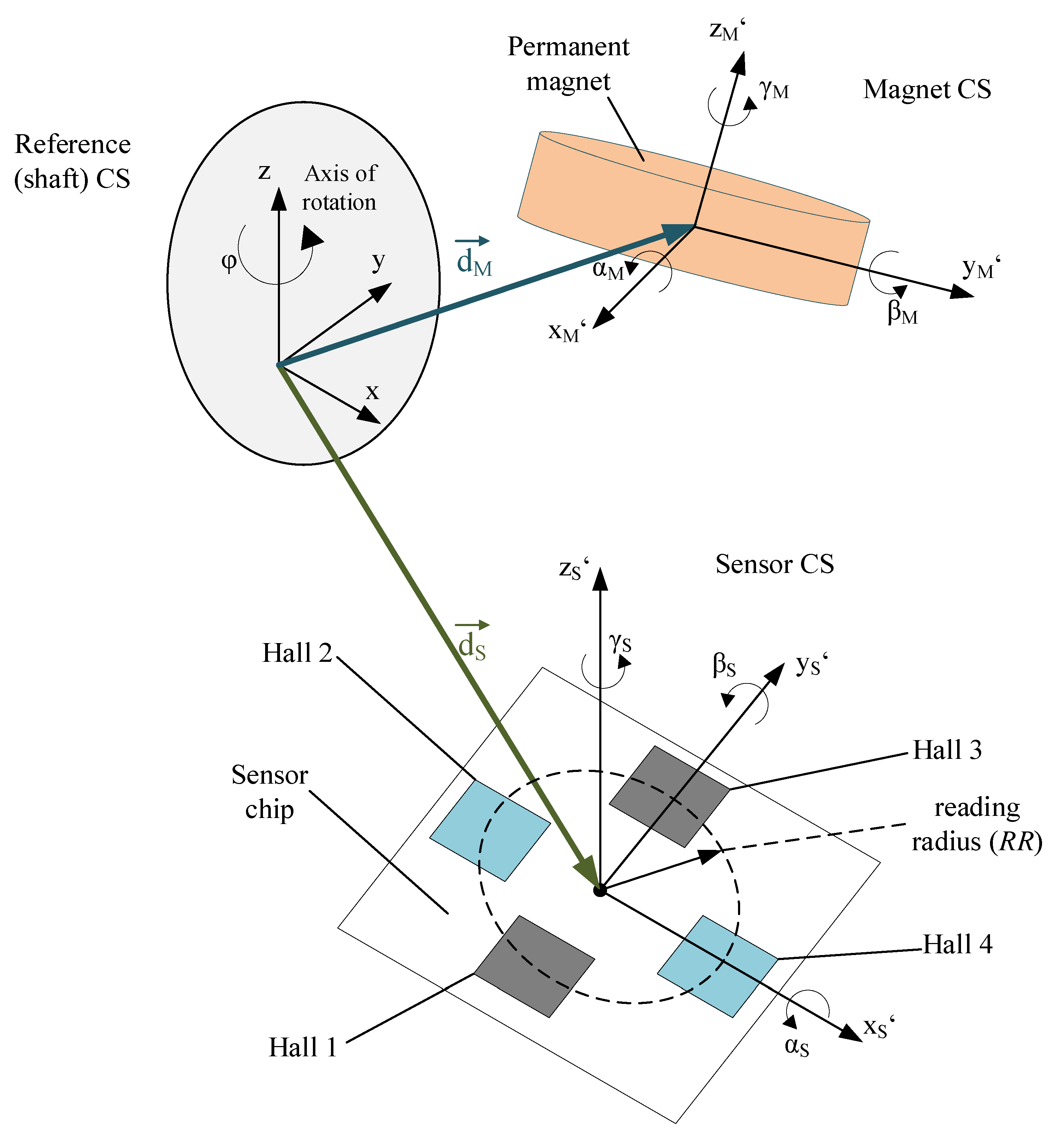
2. Methods
2.1. Magnetic Field Solution
2.2. Performing Monte Carlo Simulations
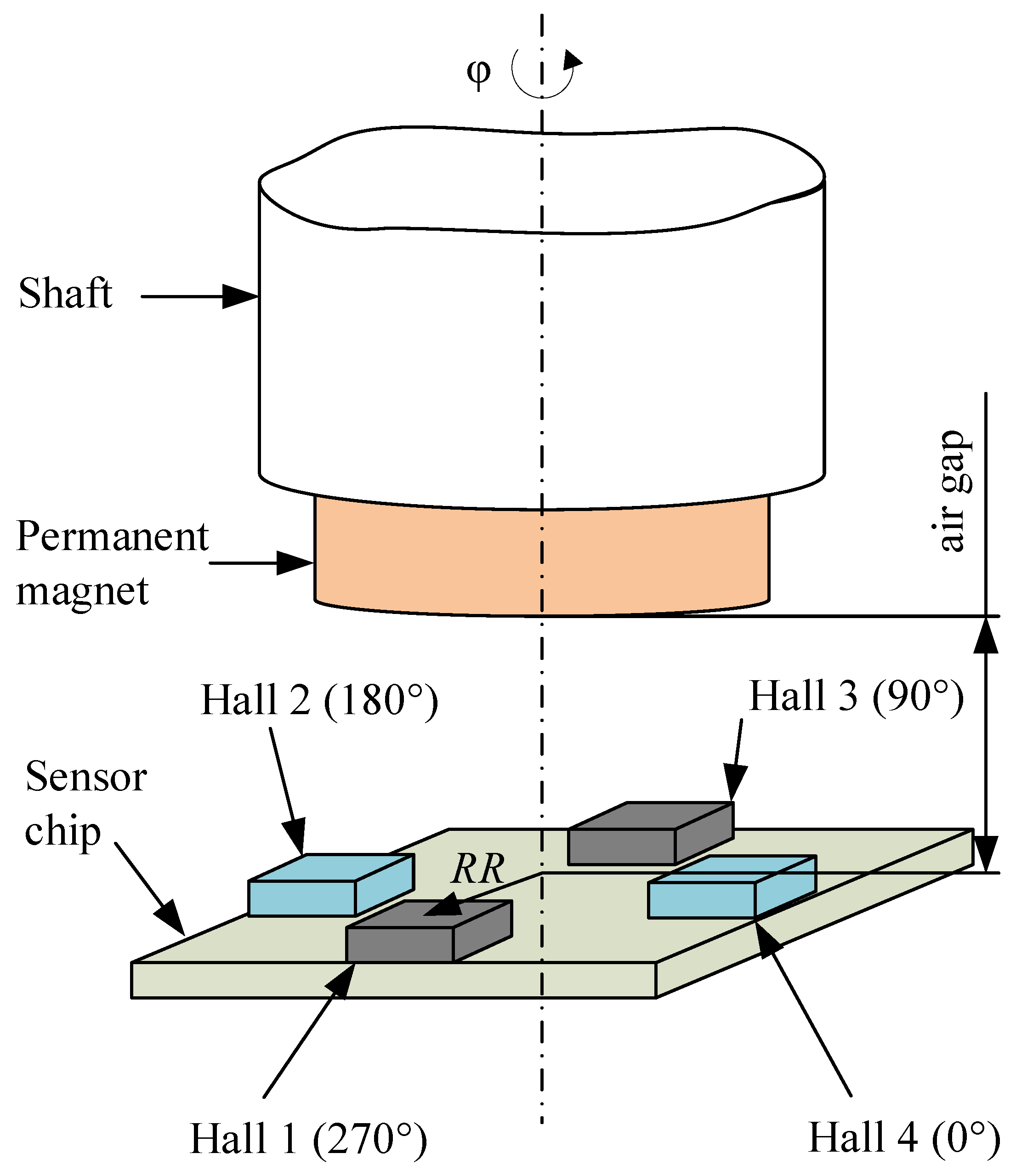
3. Model Input
- Diameter mm
- Height mm
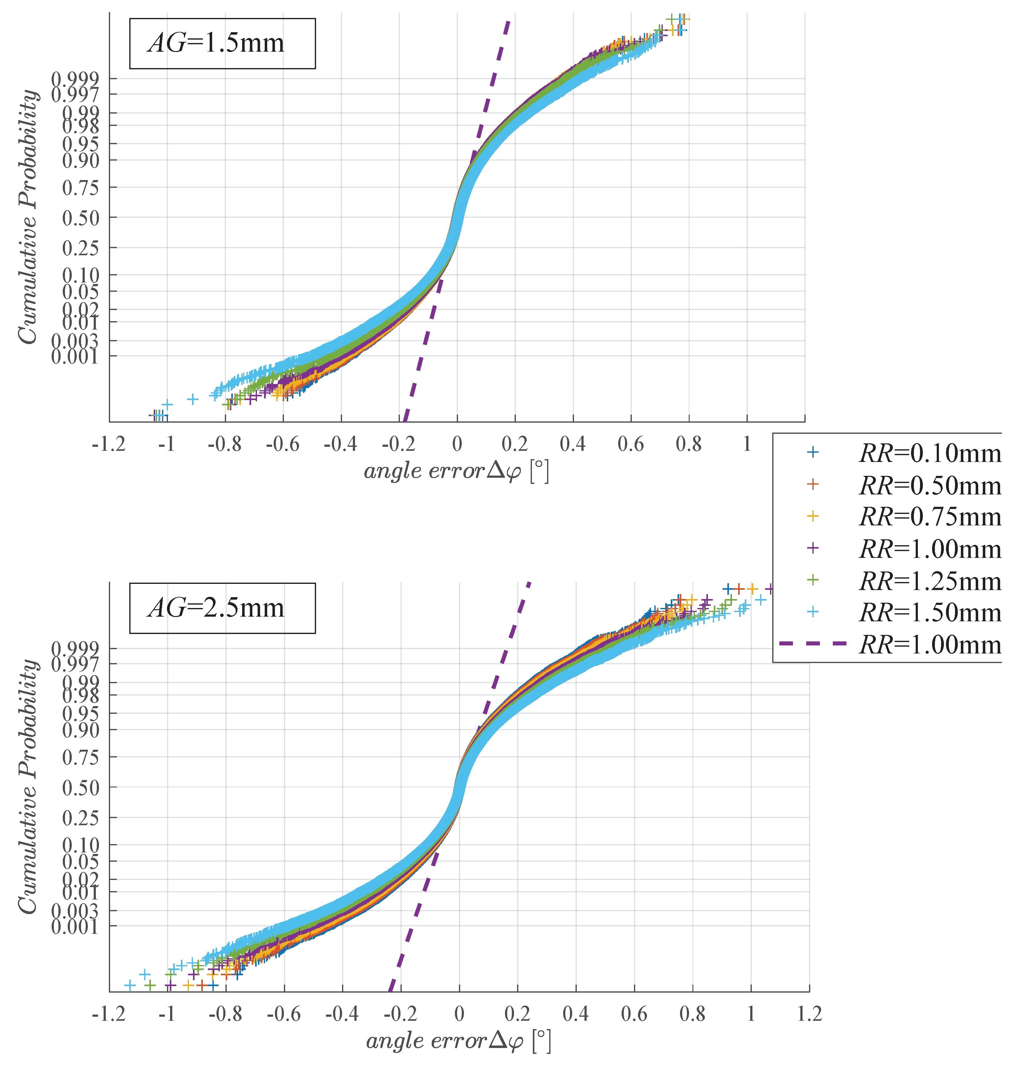
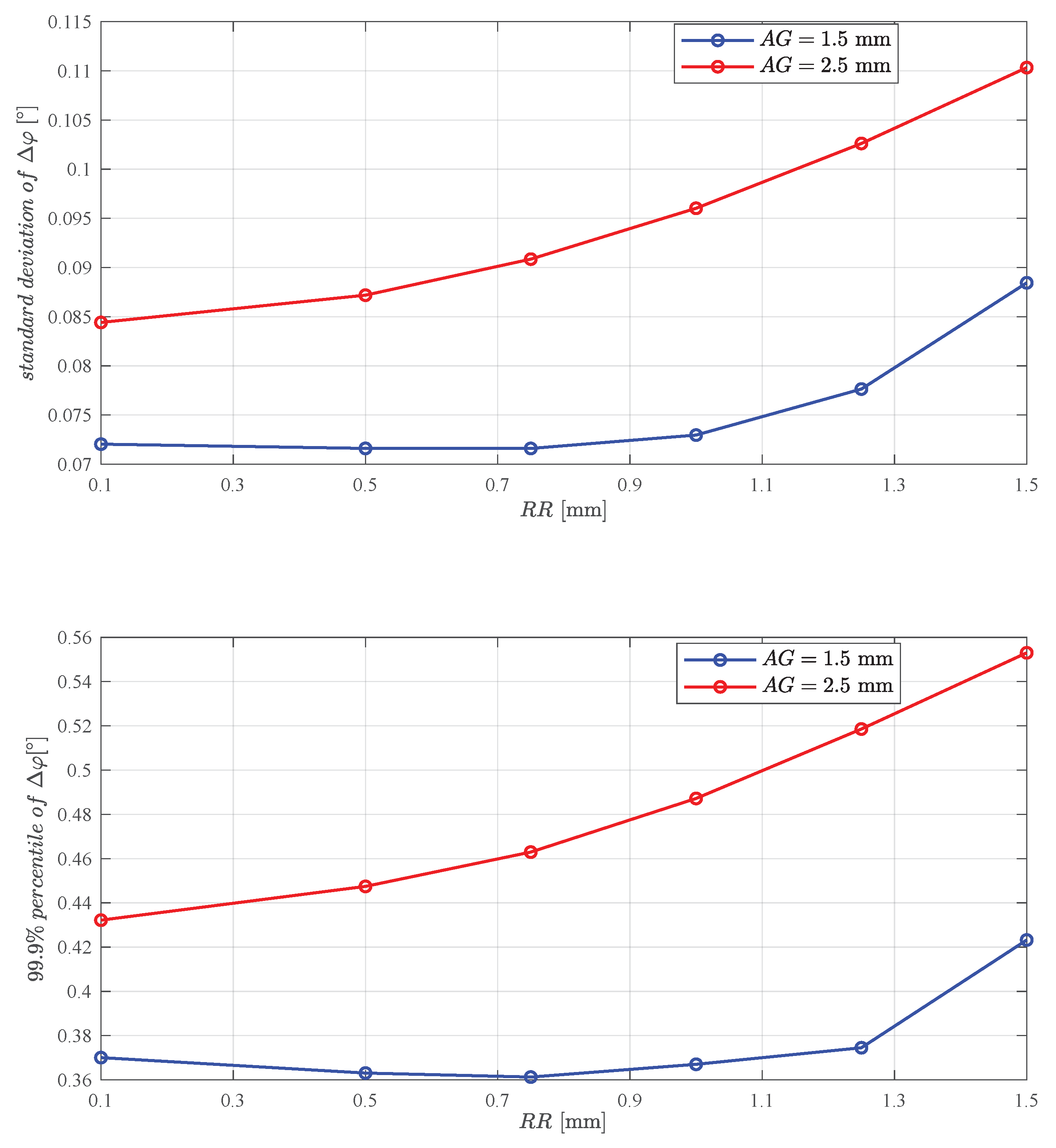
4. Results
5. Discussion
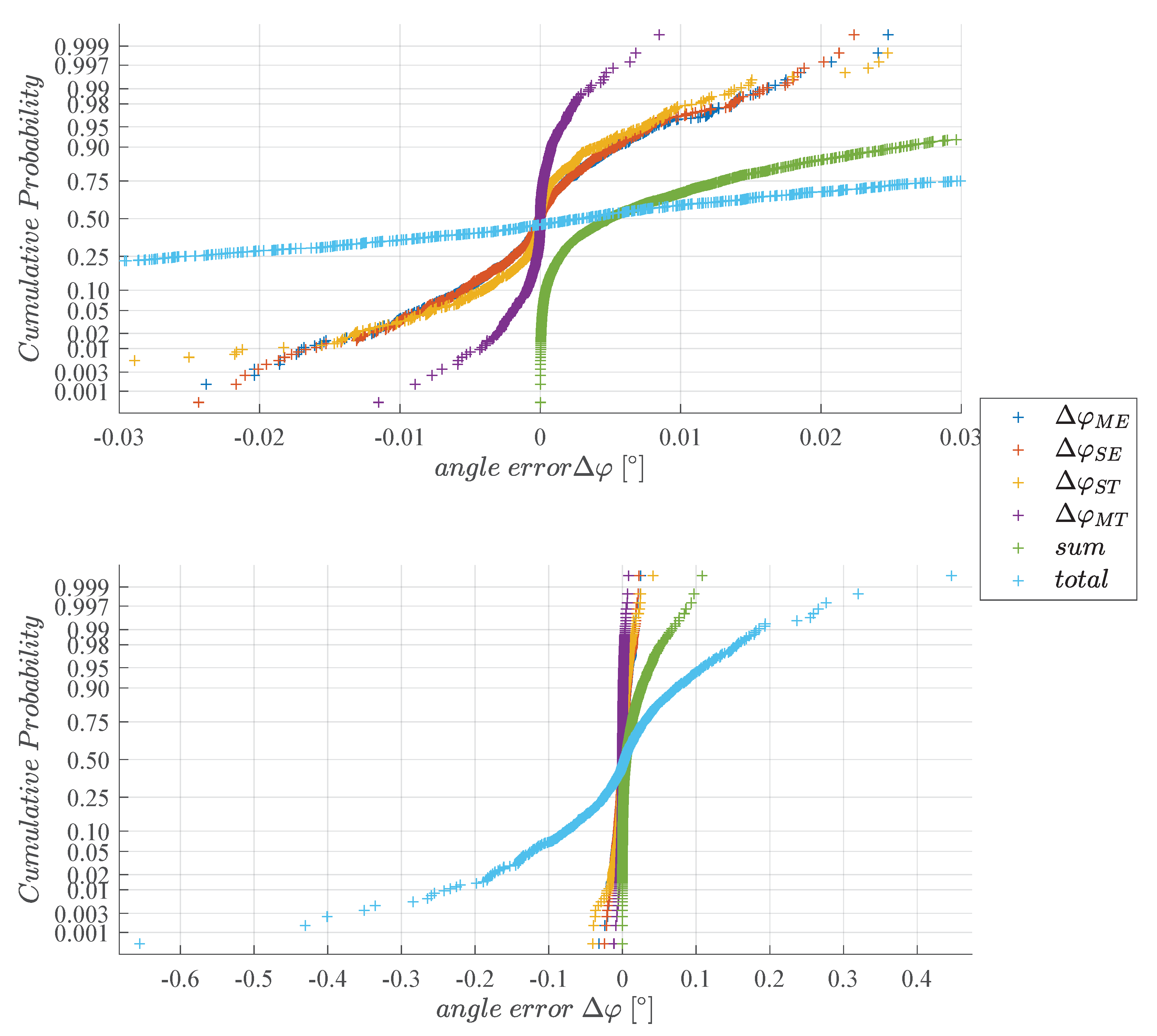
- The distribution of is clearly non-Gaussian: The angle errors of rare outliers are much bigger than one would predict with a Gaussian. Non-Gaussian error distributions have also been reported for MEMS based inclinometers by [23].
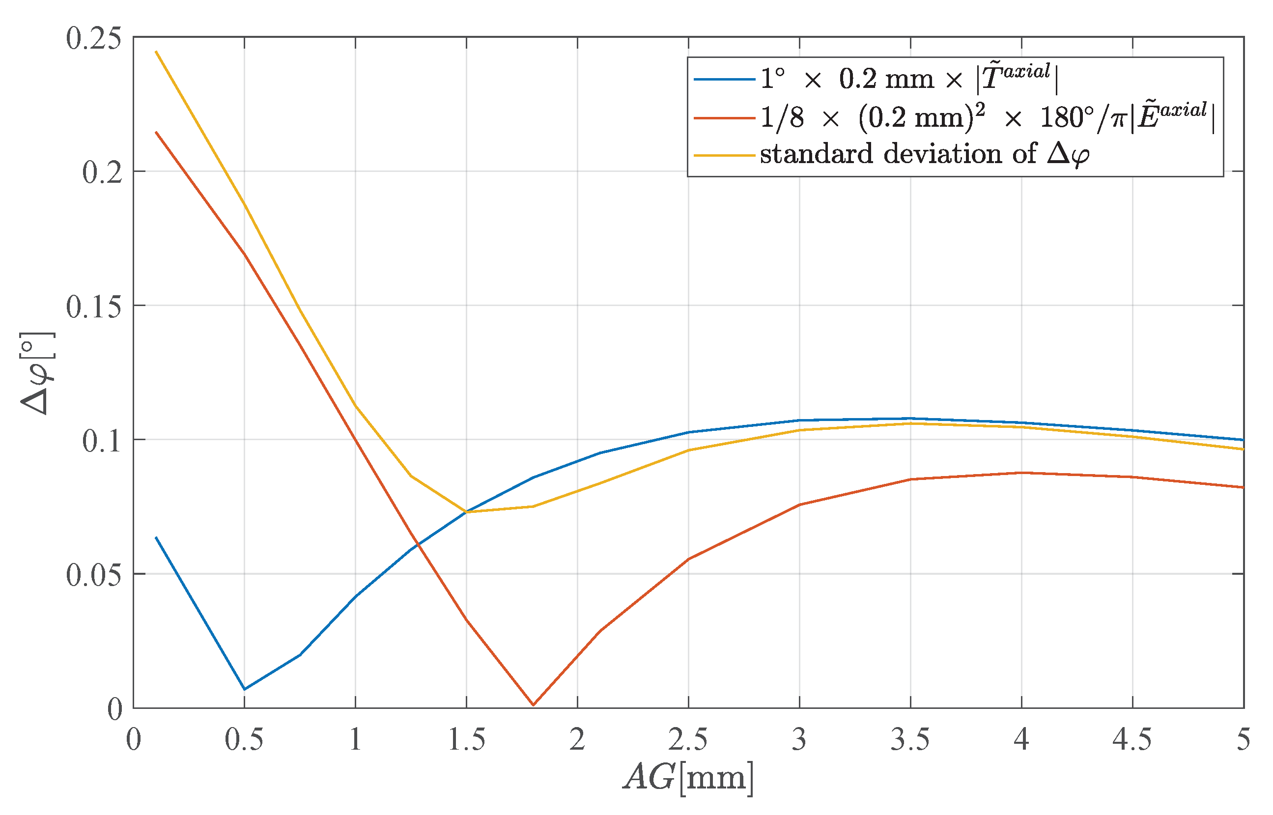
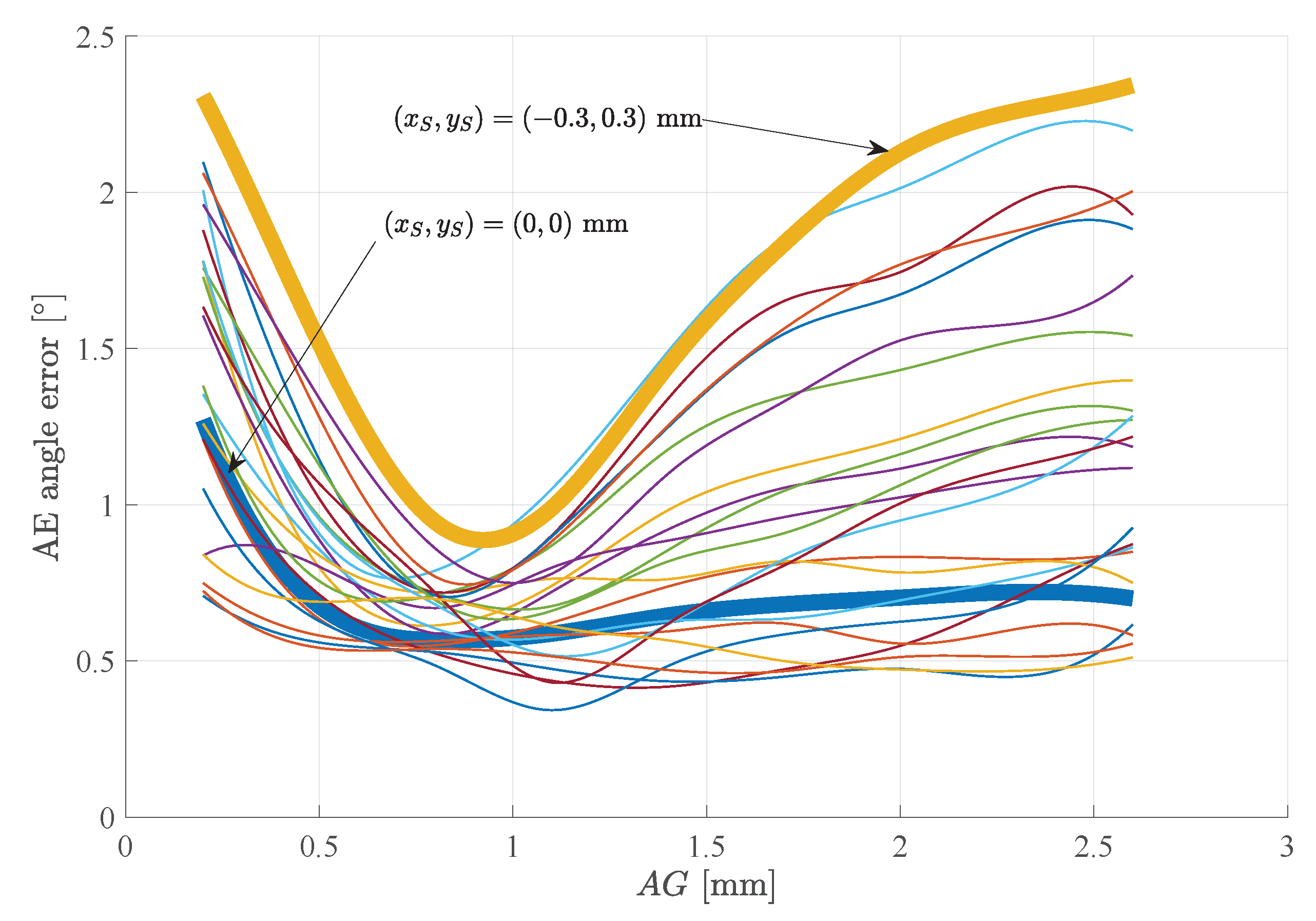
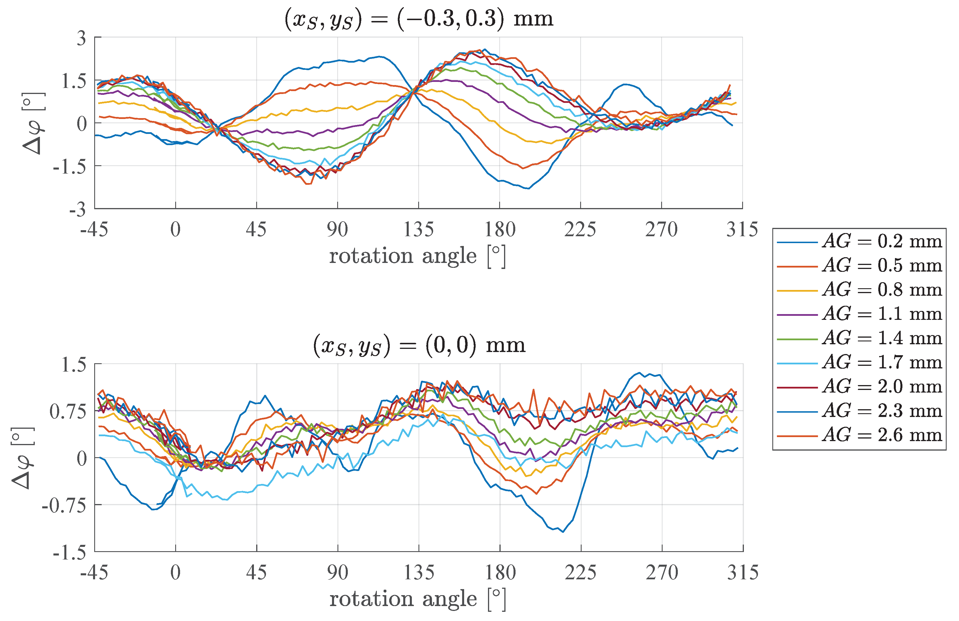
- A variation of the reading radius has less influence on than assembly tolerances.
- Typical angle errors (= standard deviation) and rare outliers ( percentiles) are similarly affected by , whereby small give slightly smaller angle errors.
| worst case angle error if only the magnet is placed eccentrically | |
| worst case angle error if only the sensor is placed eccentrically | |
| worst case angle error if only the magnet is tilted | |
| worst case angle error if only the sensor is tilted |
6. Conclusions
Author Contributions
Funding
Conflicts of Interest
Abbreviations
| AE | Average Angle Error: - /2 |
| AG | Air gap |
| Remnant magnetization | |
| D | Magnet diameter |
| DoF | Degree(s) of Freedom |
| EMI | Electromagnetic Interference |
| H | Magnet height |
| Magnetic coercivity | |
| GMR | Giant Magnetoresistance |
| MDPI | Multidisciplinary Digital Publishing Institute |
| ME | Maximum Angle Error: |
| MEMS | Microelectromechanical Systems |
| TMR | Tunnel Magnetoresistance |
| RR | Reading Radius |
| w.r.t. | with respect to |
Appendix A
- Diameter mm
- Height mm

Appendix B
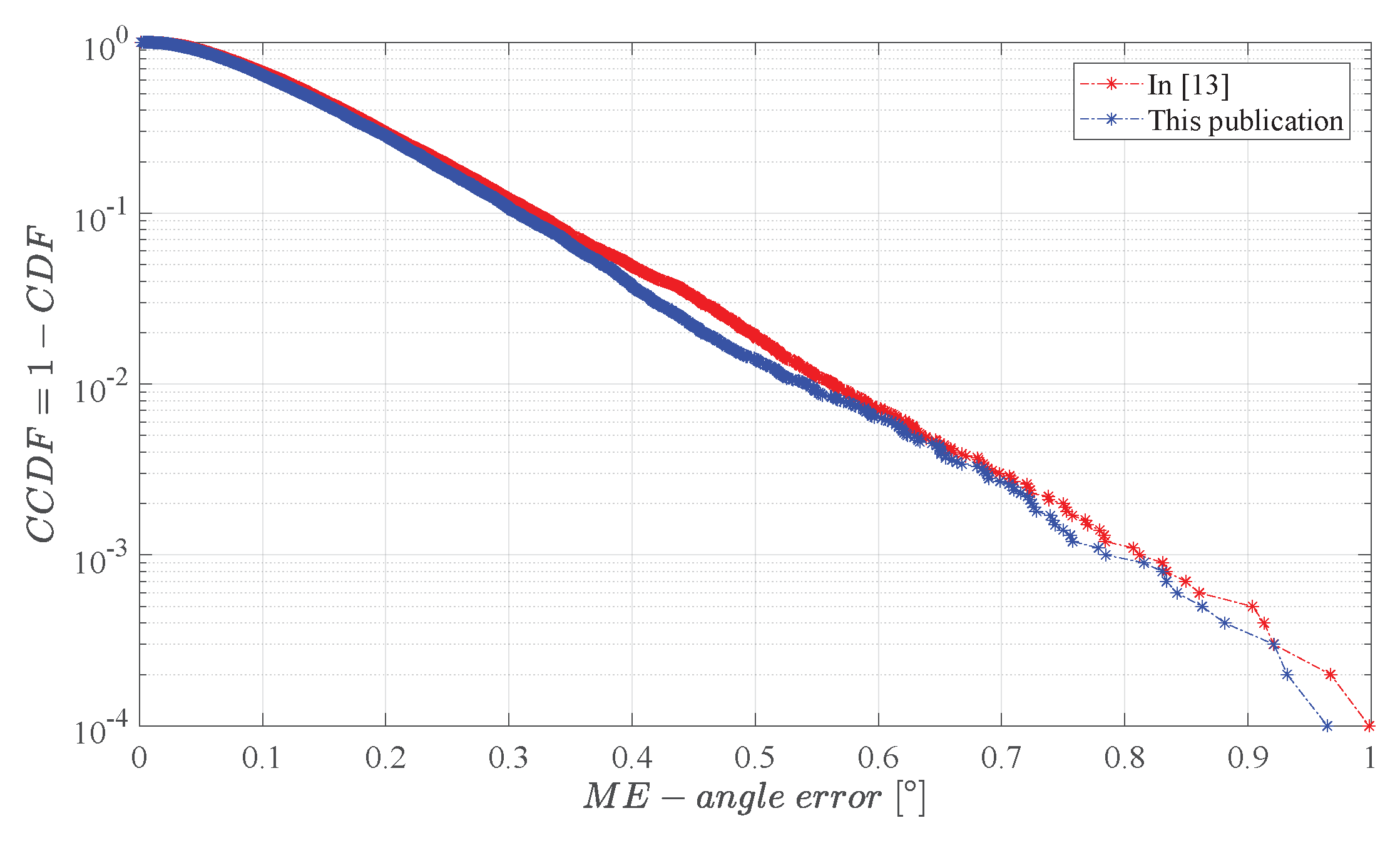
| This Publication | In [13] |
|---|---|
Appendix C
References
- Granig, W.; Hartmann, S.; Köppl, B. Performance and Technology Comparison of GMR versus commonly used Angle Sensor Principles for Automotive Applications. SAE Trans. 2007, 116, 29–41. [Google Scholar] [CrossRef]
- Granig, W.; Kolle, C.; Hammerschmidt, C.D.; Schaffer, B.; Borgschulze, R.; Reidl, C.; Zimmer, J. Integrated Gigant Magnetic Resistance based Angle Sensor. In Proceedings of the 2006 IEEE Sensors, Daegu, Korea, 22–25 October 2006; Volume 1. [Google Scholar]
- Granig, W.; Weinberger, M.; Reidl, C.; Bresch, M.; Strasser, M.; Pircher, G. Integrated GMR Angle Sensor for Electrical Commutated Motors including Features for Safety Critical Applications. In Proceedings of the Eurosensors XXIV, Linz, Austria, 5–8 September 2010; Volume 1. [Google Scholar]
- Ausserlechner, U. Inaccuracies of Giant Magneto-Resistive Angle Sensors Due to Assembly Tolerances. IEEE Trans. Magn. 2009, 45, 2165–2174. [Google Scholar] [CrossRef]
- Ausserlechner, U. The optimum layout for giant magnetoresistive angle sensors. IEEE Sens. J. 2010, 10, 1571–1582. [Google Scholar] [CrossRef]
- Ausserlechner, U. Inaccuracies of anisotropic magneto-resistance angle sensors due to assembly tolerances. IEEE Sens. J. 2012, 10, 1571–1582. [Google Scholar] [CrossRef]
- Slama, P.; Aichriedler, L. Hoch performante Rotorlage-Sensorik für bürstenlose E-Maschinen in Hybridantrieben. In Automobil-Sensorik: Ausgewählte Sensorprinzipien und deren automobile Anwendung; Tille, T., Ed.; Springer: Berlin/Heidelberg, Germany, 2016; pp. 233–250. [Google Scholar] [CrossRef]
- Metz, M.; Häberli, A.; Schneider, M.; Steiner, R.; Maier, R.; Baltes, H. Contactless Angle Measurement Using Four Hall Devices on Single Chip. In Proceedings of the International Solid State Sensors and Actuators Conference (Transducers ’97), Chicago, IL, USA, 19 June 1997; pp. 385–388. [Google Scholar]
- Kaulberg, T.; Bogason, G. An Angledetector based on magnetic sensing. In Proceedings of the IEEE International Symposium on Circuits and Systems—ISCAS ’94, London, UK, 30 May–2 June 1994; pp. 329–332. [Google Scholar]
- Kawahito, S.; Takahashi, T.; Nagano, Y.; Nakano, K. A CMOS rotary encoder system based on magnetic pattern analysis with a resolution of 10b per rotation. In Proceedings of the 2005 IEEE International Digest of Technical Papers, Solid-State Circuits Conference, San Francisco, CA, USA, 10 February 2005; pp. 240–596. [Google Scholar]
- Popovic, R.S.; Drljaca, P.; Schott, C.; Racz, R. A new CMOS Hall angular position sensor (Neuer CMOS-Hall-Winkelpositionssensor. Tech. Mess. Plattf. Methoden Syst. Anwendungen Messtech. 2001, 68, 286. [Google Scholar] [CrossRef]
- Huber, S.; Burssens, J.W.; Dupre, N.; Dubrulle, O.; Bidaux, Y.; Close, G.; Schott, C. A Gradiometric Magnetic Sensor System for Stray-Field-Immune Rotary Position Sensing in Harsh Environment. Proceedings 2018, 2, 809. [Google Scholar] [CrossRef]
- Ausserlechner, U. A Theory of Magnetic Angle Sensors with Hall Plates and without Fluxguides. Prog. Electromagn. Res. B 2013, 49, 77–106. [Google Scholar] [CrossRef]
- Francis, L.A.; Poletkin, K. Magnetic Sensors and Devices: Technologies and Applications; CRC Press: London, UK, 2017. [Google Scholar]
- Kamencky, P.; Horsky, P. An inductive position sensor ASIC. In Analog Circuit Design; Springer: Dordrecht, The Netherlands, 2008; pp. 33–53. [Google Scholar]
- Husstedt, H.; Ausserlechner, U.; Kaltenbacher, M. In-Situ Analysis of Deformation and Mechanical Stress of Packaged Silicon Dies With an Array of Hall Plates. IEEE Sens. J. 2011, 11, 2993–3000. [Google Scholar] [CrossRef]
- Furlani, E. A three-dimensional field solution for axially-polarized multipole discs. J. Magn. Magn. Mater. 1994, 135, 205–214. [Google Scholar] [CrossRef]
- Szymanski, J.E. Basic Mathematics for Electronic Engineers: Models and Applications; Taylor & Francis: London, UK, 1989; p. 154. [Google Scholar]
- Hanson, J. Rotations in Three, Four, and Five Dimensions. Available online: https://arxiv.org/abs/1103.5263 (accessed on 11 September 2019).
- James, R.C. Mathematics Dictionary; Springer Science & Business Media: Berlin, Germany, 1992; p. 424. [Google Scholar]
- MathWorks Inc. Matlab Online Documentation- Normrnd. Available online: https://de.mathworks.com/help/stats/normrnd.html?s_tid=doc_ta (accessed on 7 August 2019).
- MathWorks Inc. MATLAB Online Documentation-Rand. Available online: https://de.mathworks.com/help/matlab/ref/rand.html?s_tid=doc_ta (accessed on 7 August 2019).
- Schmidt, R.; O’Leary, P.; Ritt, R.; Harker, M. MEMS Based Inclinometers: Noise Characteristics and Suitable Signal Processing. In Proceedings of the 2017 IEEE International Instrumentation and Measurement Technology Conference (I2MTC), Turin, Italy, 22–25 May 2017. [Google Scholar]
- Ausserlechner, U. Magnet Arrangement and Sensor Device. U.S. Patent US020170241802A1, 24 August 2017. [Google Scholar]


| Sensor DoF | Magnet DoF |
|---|---|
| Position () | Position () |
| Orientation (w.r.t. shaft CS) | Orientation (w.r.t. shaft CS) |
| Sensor Tolerances | Magnet Tolerances |
|---|---|
© 2019 by the authors. Licensee MDPI, Basel, Switzerland. This article is an open access article distributed under the terms and conditions of the Creative Commons Attribution (CC BY) license (http://creativecommons.org/licenses/by/4.0/).
Share and Cite
Ergun, S.; Ausserlechner, U.; Holliber, M.; Granig, W.; Zangl, H. A Statistical Investigation into Assembly Tolerances of Gradient Field Magnetic Angle Sensors with Hall Plates. Mathematics 2019, 7, 968. https://doi.org/10.3390/math7100968
Ergun S, Ausserlechner U, Holliber M, Granig W, Zangl H. A Statistical Investigation into Assembly Tolerances of Gradient Field Magnetic Angle Sensors with Hall Plates. Mathematics. 2019; 7(10):968. https://doi.org/10.3390/math7100968
Chicago/Turabian StyleErgun, Serkan, Udo Ausserlechner, Michael Holliber, Wolfgang Granig, and Hubert Zangl. 2019. "A Statistical Investigation into Assembly Tolerances of Gradient Field Magnetic Angle Sensors with Hall Plates" Mathematics 7, no. 10: 968. https://doi.org/10.3390/math7100968
APA StyleErgun, S., Ausserlechner, U., Holliber, M., Granig, W., & Zangl, H. (2019). A Statistical Investigation into Assembly Tolerances of Gradient Field Magnetic Angle Sensors with Hall Plates. Mathematics, 7(10), 968. https://doi.org/10.3390/math7100968