Risk Management for Bonds with Embedded Options

Abstract

This paper examines the behavior of the interest rate risk management measures for bonds with embedded options and studies factors it depends on. The contingent option exercise implies that both the pricing and the risk management of bonds requires modelling future interest rates. We use the Ho and Lee (HL) and Black, Derman, and Toy (BDT) consistent interest rate models. In addition, specific interest rate measures that consider the contingent cash-flow structure of these coupon-bearing bonds must be computed. In our empirical analysis, we obtained evidence that effective duration and effective convexity depend primarily on the level of the forward interest rate and volatility. In addition, the higher the interest rate change and the lower the volatility, the greater the differences in pricing of these bonds when using the HL or BDT models.

1. Introduction

The aim of this paper is to analyze and interpret interest rate risk management measures for option-embedded bonds under different specifications of interest rate dynamics. In addition, we studied the factors, on which they depend, based on the assumption that the choice of the consistent interest rate model used to price these securities can have a significant impact on the calculation of those measures. The cash flows from a callable (putable) bond depend on the possible exercise of the call (put) option, i.e., early redemption in favor of the issuer (bondholder). Therefore, the pricing of these bonds requires modelling of future interest rates from the actual term structure of interest rates and the actual term structure of volatility. We used two consistent term structures of interest rates models, the Ho and Lee (HL) [1] and Black, Derman, and Toy (BDT) [2] models. We estimated different measures of interest risk management and examine the main factors that determine their behavior, such as the interest rate volatility, the shape of the yield curve, and the changes in the yield curve. To illustrate the process, we examined the daily price behaviors of two annual coupon corporate bonds with embedded options throughout their lifetimes. These bonds were selected, because they were actively traded in a sample period that was particularly interesting for our analysis, given the dramatic changes in both the level and the slope of the term structure of interest rates.

Managing these option-embedded bonds, of which the cash flow structure depends on future interest rates, requires two additional challenges over any plain vanilla bond. On the one hand, the bond’s price in an interest rate model is needed to apply to the bond’s price. There are two different approaches to modelling the dynamics of interest rates: equilibrium models and nonarbitrage models. Both of them start from a stochastic differential equation for a short interest rate but differ in the procedure used to implement the models. Thus, equilibrium models are based on the estimation of parameters from historical data, assuming that they are constant for a given period. On the other hand, consistent models or nonarbitrage models replicate exactly the term structure corresponding to the calibration date. The latter is preferred by the financial industry over the former. Some of the most popular models among practitioners are those proposed by HL and BDT.

On the other hand, traditional bond sensitivity measures that do not incorporate options, i.e., duration and convexity, are no longer appropriate, and instead, the effective or option-adjusted duration and convexity are used. In addition, there is the concept of option-adjusted spread (OAS), which takes into account the fact that the securities contain early redemption provisions although similar to the concept of yield spread applied to the pricing of straight bonds.

In our paper, we applied the HL and BDT models in the analyses of two coupon-bearing bonds with embedded options, a callable bond and a putable bond. Both were actively traded in the Spanish corporate debt market during a broad sample period 1993–2003 and were chosen for its dramatic changes in both the level and the slope of the time structure of interest rates. This interest rate behavior makes it easier to draw conclusions from our analysis.

The main contributions of our paper are the following. Firstly, we carried out a daily analysis of the relationship between traditional interest rate risk management measures and option-adjusted measures based on the expected future evolution of interest rates at any given time, showing the attractiveness of the option to the investor. Secondly, the main factors determining the behaviors of these measures were analyzed. Finally, the implications of the choice of a model for the dynamics of interest rates and the extent of rate changes used in the calculation of effective duration (ED) and convexity were studied.

2. Bonds with Embedded Options

The two most common types of embedded options are call provisions and put provisions, so we can distinguish two main types of bonds with embedded options—callable bonds and putable bonds. A callable bond is a bond that can be redeemed by the issuer before its maturity date, and a putable bond can be sold by the bondholder before its maturity date. A callable bond allows its issuer to repurchase its debt at par value before maturity in the event that interest rates fall below the issue’s coupon rate or its credit rating improves. In both cases, the issuer has the opportunity to issue a new bond at a lower coupon rate. This is a disadvantage for the investor. In the event of early redemption, the investor will be paid the price at par, far below the price of an equivalent straight bond, and will have to reinvest in another bond at a time when interest rates are lower than the coupon rate of the original issue. Hence, buying a callable bond comes down to buying an option-free or plain vanilla bond and selling a call option to the issuer of the bond. The value of a callable bond can be estimated from the price of an identical straight bond minus the value or premium of the embedded call option sold.

A putable bond allows its holder to sell the bond at a face value before maturity, in case that interest rates exceed the issue coupon rate. This gives you the opportunity to buy a new bond with a higher coupon rate. The purchase of a putable bond comes down to buying an option-free bond as well as a put option. The price of the putable bond is the price of an identical straight bond plus an embedded put option purchased. The embedded option can be exercised from a specific date on (American option) or on a specific date (European option), depending on the bond, at the strike price.

Unlike an option-free straight bond, an embedded option bond is a contingent claim, i.e., its future cash flows are uncertain, because they depend on the future value of interest rates. To price such a bond, it is necessary to use a model that explains the fact that future interest rates are uncertain. This uncertainty is described by the term structure of the volatilities of the relative changes in interest rates. The most commonly used method for pricing these bonds is the binomial interest tree model.

3. Consistent Interest Rate Models

The HL model is the first consistent term structure of an interest rates model and is presented as an alternative to equilibrium models [3,4]. It proposes a general methodology to price a wide range of interest rates contingent claims. The model is presented in the form of a binomial bond price tree with two parameters—the volatility of the short interest rate and the market price of the short rate risk. The inputs of the model are the yield curve and the short rate volatility. The main limitation is that interest rates are normally distributed, so we can get negative values.

The short-interest-rate dynamic dr in the continuous time version can be represented by Equation (1):

$$dr=\theta \left(t\right)dt+\sigma dz,$$

(1)

where σ is the instantaneous standard deviation of the short rate, r is a constant, θ(t) is the drift of the process, and z is a standard Wiener process.

The drift θ(t) is chosen so as to exactly fit the term structure of interest rates being currently observed in the market. It depends on the time t, on the slope of the instantaneous forward curve in 0, f(0, t), and on the constant short rate volatility, σ. The drift θ(t) can be written as:

$$\theta \left(t\right)=\frac{\partial f\left(0,t\right)}{\partial t}+{\sigma }^{2}t.$$

(2)

The BDT model assumes that interest rates follow a lognormal distribution. This model has the advantage over the HL model, i.e., the interest rate cannot become negative. The equivalent stochastic process corresponding to the model is described as:

$$d\ln r=\left[\theta \left(t\right)+\frac{{\sigma }^{\prime }\left(t\right)}{\sigma \left(t\right)}\ln r\right]dt+\sigma \left(t\right)dz,$$

(3)

where $\theta \left(t\right)$ and $\sigma \left(t\right)$ are two independent functions of time chosen so that the model fits the term structure of spot interest rates and the term structure of spot rate volatilities.

Both models are implemented using their original discrete version through binomial trees. These trees are calibrated from the previously estimated zero-coupon yield curve and the historical term structure of interest rate volatility for each maturity. The calibration process requires the joint adjustment of several binomial trees. We followed the method proposed by [5]. The main output of the process is the short-term interest rate at each time, t, and interest state, i. State prices can be obtained from the trees. State-contingent claims are securities that pay off in some interest rate states, but not in others. Thus, each state price is the current value of $1 received at a given interest rate state and a given time in the future. If the option has been exercised in this node, state security pays nothing.

For the sake of brevity, the calibration process is not described. By way of illustration, here are some basic ideas about the procedure in the case of the BDT model. We followed the forward process developed by [6] that proves that the level of the short rate in t can be estimated from Equation (4):

$$r\left(t\right)=U\left(t\right)exp(\sigma \left(t\right)z\left(t\right)),$$

(4)

where U(t) is the median of the log short rate distribution in t, σ(t) is the short rate volatility, and z(t) represents a Brownian motion.

Although most practitioners make extensive use of a simplification of the BDT model assuming constant interest rate volatility, we used the original version. The term structure of the volatility was calibrated from Equation (5):

$$\sigma \left(i\right)\sqrt{\Delta t}=\frac{1}{2}ln\frac{r_U\left(i\right)}{r_D\left(i\right)},$$

(5)

where Δt is the width of each of the time steps, into which the bond’s term to maturity is divided, σ(i) is the interest rate volatility at the interest state i with i being each of the possible interest rate nodes for term t, $r_U\left(i\right)$ and $r_D\left(i\right)$ are the short interest rates as seen from the nodes U and D, respectively. $P_U\left(i\right)$ and $P_D\left(i\right)$ are the corresponding discount functions, i.e., the prices of zero-coupon bonds, when interest rates rise and fall, respectively, which can be written as:

$$P_D\left(i\right)=P_U{(i)}^{exp(-2\sigma \left(i\right)\sqrt{\Delta t})}.$$

(6)

The calibration process is carried out for each of the dates [7], on which each of the two coupon-bearing bonds analyzed is traded throughout its life cycle. We used daily estimates of the zero-coupon yield curve as inputs in the calibration process, which we previously estimated via a weighted version of the Nelson and Siegel model [8] (see [9,10]). We assumed a heteroskedastic price error scheme, and a generalized least square (GLS) method was employed. The data in the previous analysis were the Spanish Treasury bill and bond prices of all actual transactions from the sample period. These daily term structures of interest rates and the historic term structures of volatilities were used to calibrate the binomial trees for the short rate with monthly time steps.

4. Interest Rate Risk Measures

The behaviors of callable and putable bonds were analyzed by taking into account their risk arising from changes in the underlying variables, such as volatility or yield curve changes. Traditional interest rate risk measures, modified duration (MD) and convexity, are not suitable for option-embedded bonds, because they do not consider the possibility of option exercise. Instead, ED is defined as a rough measure of the sensitivity of the bond’s price to changes in interest rates. More specifically, it is the percentage change in the bond’s price to a parallel shift in the yield curve by a certain number of basis points (Δy). Effective convexity (EC) approximates the second derivative of the bond price function with respect to the yield curve. This concept is useful, when a portfolio manager expects a potentially large shift in the term structure. The calculation of these measure requires the estimation from the current price P₀ of prices in the case of declining (P_D) and increasing (P_U) interest rates. ED can be calculated as follow:

$$ED=\frac{P_D-P_U}{2P_0\left(\Delta y\right)}.$$

(7)

EC was given by Equation (8):

$$EC=\frac{P_D+P_U-2P_0}{2P_0{(\Delta y)}^2}.$$

(8)

To estimate these interest risk management measures, we followed the procedure described in [8,9]. We recalibrate the HL and BDT models after shifting the Treasury yield curve by ±25 and ±100 bp. In addition, we calculated the OAS for each date. The OAS is the constant spread, which equalizes the theoretical price of a bond at its market price when added to all the short-term interest rates on the binomial tree.

5. Sample Description and Estimation Procedure

In order to meet our objectives, we chose a sample period with strong changes in the term structure of interest rates, in which default risk hardly changed. The Spanish fixed-income market, both corporate and government, during the period 1993 to 2004 was particularly suitable. The first part of the sample was characterized by strong monetary tensions, including currency devaluations, and sharp and severe interest rate swings. The slope of the yield curve went from rising to falling. Subsequently, there were sharp reductions in levels to meet the convergence criteria to ensure entry into the single currency. The final part of the sample was characterized by a surge in interest rates in 2001. We examined the two most actively traded corporate bond issues with embedded options in the Spanish corporate fixed-income market AIAF during the period. One issue contained a call option, and the other included a put option. Both were European options.

Table 1. Main features of the issues, i.e., Banco de Crédito Local (BCL) and Túnel del Cadí (TC).

Bond Characteristics	BCL	TC
Issuance date	14 December 1993	31 May 1994
Maturity date	1 July 2003	31 May 2004
Annual coupon rate (%)	8.4	9.85
Outstanding amount	€178 million	€48 million
Rating	Aa3	No rated
Percentage of traded days (%)	9.5%	5.1%
Daily trading volume	€6.5 million	€1.0 million
Type of option	Call (European)	Put (European)
Option exercise price (%)	100	100
Option exercise date	1 July 1998	31 May 2000
# Observations up to exercise date	106	101
# Observations	106	128

describes the main features of the issues.

As mentioned, we calibrated the HL and BDT models to the Spanish Treasury yield curve. Estimates of the term structure of interest rates were made from the daily trading of Spanish Treasury debt securities using the Nelson and Siegel duration-weighted model.

To calculate sensitivity measures for bonds with embedded options, we applied the following steps [11,12]. First, we calculated the theoretical price of the bonds from the HL and BDT yield curve models. Second, we obtained the OAS for all days, of which issues were traded during the period 1993–2004. Third, we shifted the on-the-run yield curve up and down by ±25 and ±100 bp and constructed new binomial interest rate trees. Fourth, we added a constant OAS to each node of the new interest rates trees. Fifth, we used the adjusted trees to determine the value of bonds, from which we calculated ED using Equation (7) and EC using Equation (8).

In addition, we computed for the entire sample period of the MD and convexity assuming two possibilities. In the first case, the option was not exercised, so we had the MD- and convexity-to-maturity. In the second one, we supposed that the option was exercised, so we had the MD- and convexity-to-call/put. We compared these new measures with ED and EC.

6. Results

Figure 1 shows graphically the estimates of ED calculated from each of the two consistent models, HL and BDT. In the calculation of ED, we used a parallel variation of ±100 bp along the entire yield curve. The top line shows the MD-to-maturity, i.e., assuming an option-free bond. The lower line represents the MD to the date of the option exercise and was calculated assuming that the option was exercised for certain (MD-to-call or MD-to-put). On dates, when the bond was not traded and there was no market price, we obtained a theoretical price, based on which the MD was estimated. We assumed that the bond’s yield-to-maturity (YTM) was the spot interest rate provided by the yield curve for the term to maturity (top line) or to the exercise date (bottom line) on that date plus the average OAS of the issue over its life (55 bp for the Banco de Crédito Local (BCL) and 126 bp for the Túnel del Cadí (TC)). This YTM made it possible to obtain the theoretical price of the bond for each date and the MD for each interest rate model.

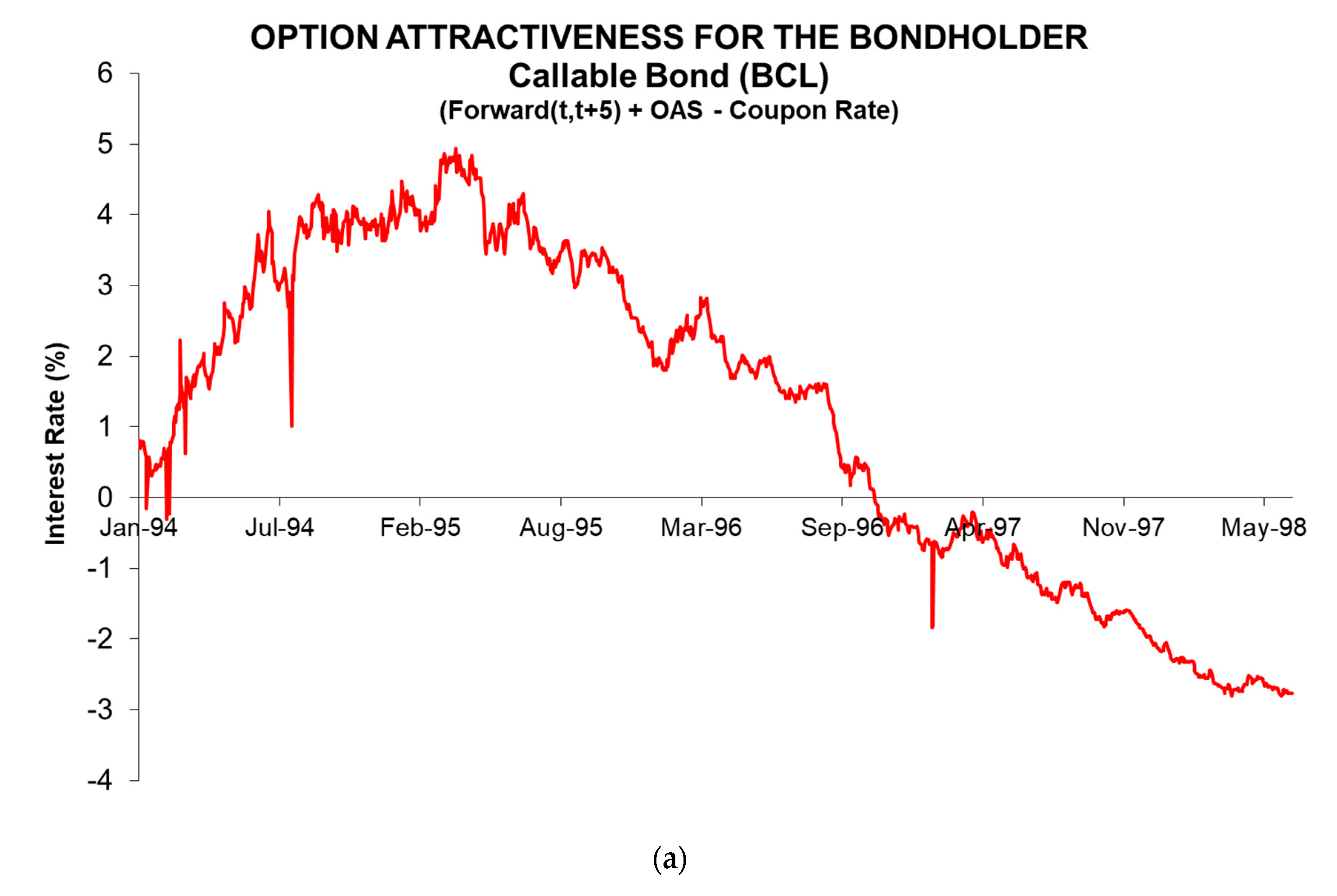
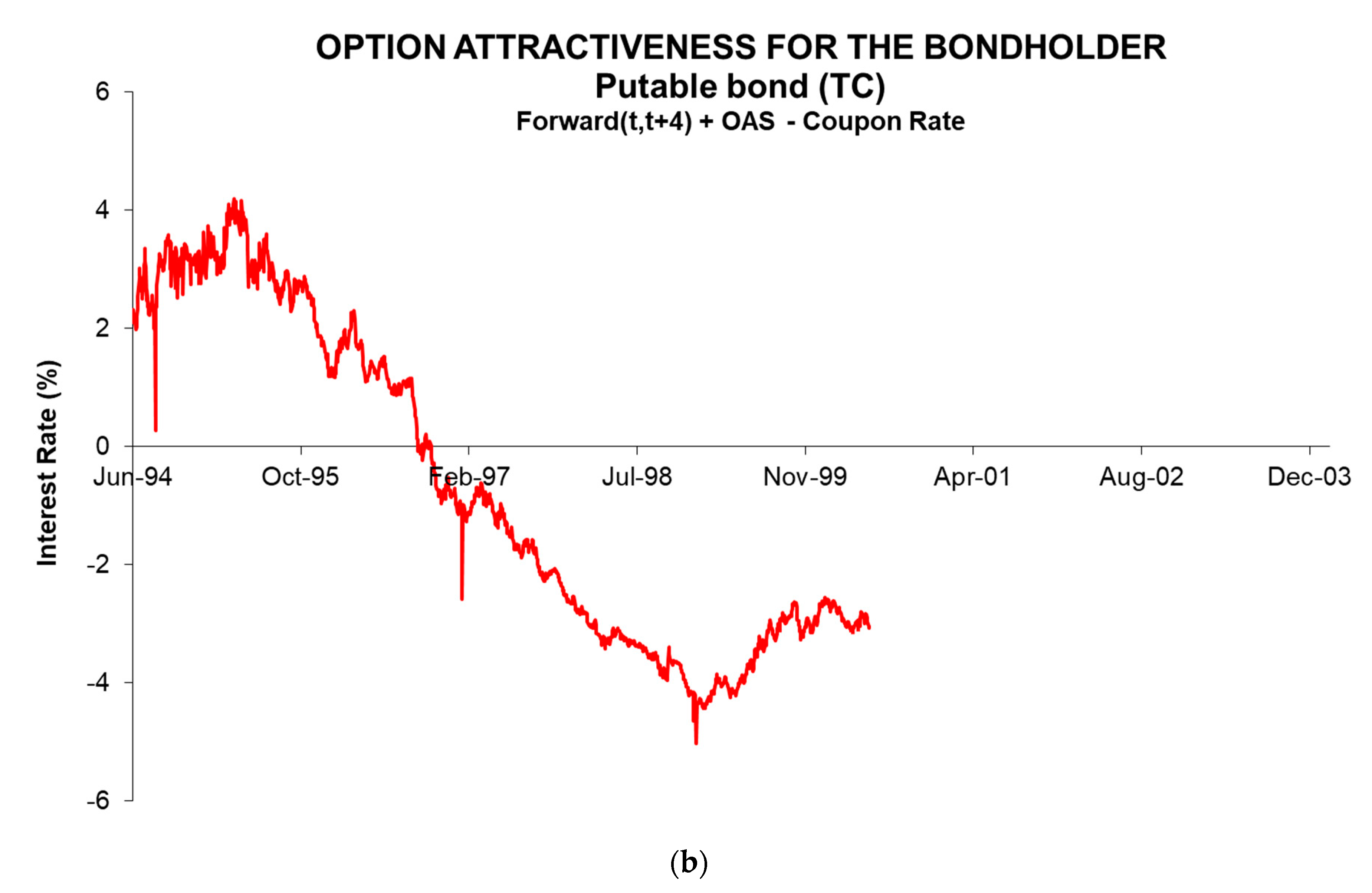
The price of bonds with embedded options depends on investors’ expectations about the possible future exercise of the option. If future interest rates that are deducted from the current yield curve, i.e., forward rates, indicate that they will remain above the bond’s coupon rate, the possibility of call exercise will be remote and the price of the callable bond will be slightly lower than a similar nonoption bond. In contrast, the price of a putable bond should be well above that of a similar straight bond. Expectations of future interest rate behavior are key in pricing these bonds. This is how we proposed the variable, option attractiveness (OA), for the bondholder. It was calculated from Equation (9):

Option attractiveness = Forward (t, T) + OAS − Coupon rate,

(9)

where Forward (t, T) is the prediction, assuming the expectative theory is true, of future interest rates for the period between the strike date t and the maturity date T. Hence, for callable bonds, the option is attractive when the OA gets negative values, while for putable bonds the option is attractive when the OA is positive.

Figure 2 shows the time evolution of the OA from the point of view of the bondholder. It can be seen that the OA of the callable issue, BCL, was positive for a large part of the sample, which indicated a few possibilities of exercise that were corroborated by an ED, which was very close to the MD-to-maturity (top line in Panel (a) of Figure 1). As of mid-1996, the OA became negative, at which point the exercise of the call became probable. At the dates, when the bond was traded in 1998, the market took the call exercise for granted. In that period, the ED practically coincided with the MD-to-call (bottom line in Panel (a) of Figure 1). The behavior of the putable bond, TC, was completely different (Panel (b) of Figure 2). From the beginning of the sample, the evolution of interest rates pointed to a probable exercise of the put option, as they were above the coupon rate. The ED in that period was between the two MD limits, i.e., the MD-to-maturity (upper line) and the MD-to-put (lower line). However, as a result of persistent rate falls, from the third quarter of 1996, interest rates were well below the coupon rate and the ED was virtually the same as the MD-to-maturity, so that the early repayment clause was worthless. The put option expired without being exercised, and the bond was redeemed at maturity. In view of the above results, the OA measure and the ED’s position with regard to the MD thresholds clearly showed the possibilities to exercise the options embedded in the bonds.

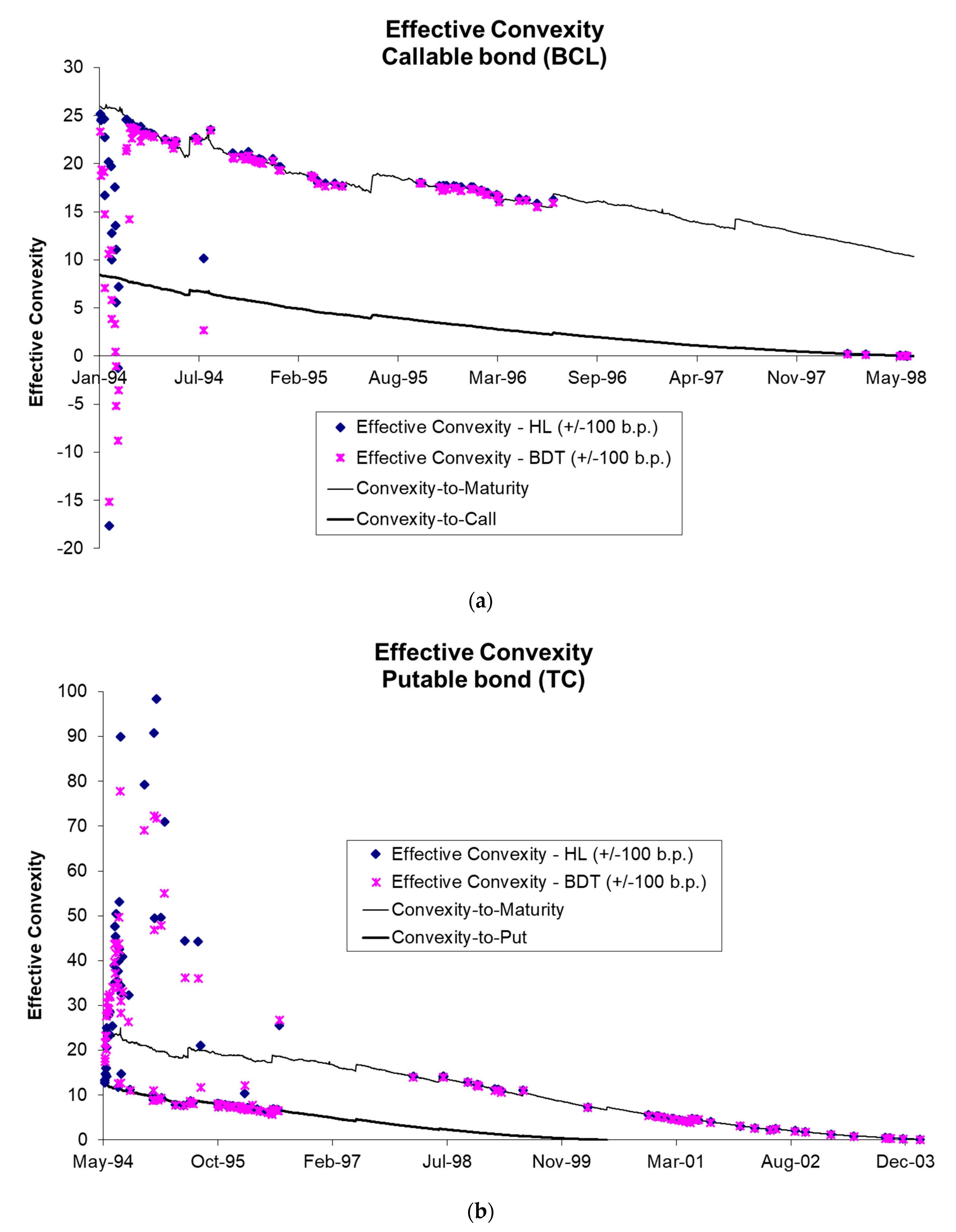
We represent the EC in Figure 3, and we can see a similar pattern for the results. As in the ED analysis, we estimated two thresholds, between which the EC had to be situated, the convexity until maturity and the convexity until the date of the exercise of the option. However, the phenomenon known as “price compression” made it possible for the EC to occasionally be outside these thresholds. Figure 3a,b shows that in the first few days of trading there was great instability in estimates as a result of the extreme movements in the level and slope of the yield curve. The call option put a ceiling on the price of callable bonds, and the put option put a floor on putable bonds. This ceiling/floor pushed the EC outside the thresholds of convexity calculated for an option-free bond. Another aspect to be highlighted in this analysis was the large differences observed in the estimated EC according to the interest rate model used in its estimation. Logically, these differences had significant implications for risk management of these issues.

Table 2. Differences between the HL and BDT models in terms of ED, EC, and option price. These differences were calculated as the value of the variable obtained using the HL model minus the value of the variable obtained using the BDT model.

Type of Bond	Differences in ED (the Value Obtained by the HL Model—the Value Obtained by the BDT Model) for a ±25 bp Change in the Yield Curve	Differences in ED (the Value Obtained by the HL Model—the Value Obtained by the BDT Model) for a ±100 bp Change in the Yield Curve	Differences in EC (the Value Obtained by the HL Model—the Value Obtained by the BDT Model) for a ±25 bp Change in the Yield Curve	Differences in EC (the Value Obtained by the HL Model—the Value Obtained by the BDT Model) for a ±100 bp Change in the Yield Curve	Differences in Option Price (the Value Obtained by the HL Model—the Value Obtained by the BDT Model)
Callable bond
- Average	0.0388	0.0490	1.4863	1.6681	−0.1288
- Median	0.0373	0.0433	0.2307	0.2423	−0.1227
SD	0.0258	0.0362	3.8977	3.3989	0.1274
Putable bond
- Average	0.0062	0.0268	−0.8147	0.6357	−0.0649
- Median	0.0215	0.0284	0.0906	0.1368	−0.0535
SD	0.0736	0.0511	20.0785	5.0451	0.0463

shows some statistics of the differences in risk management measures calculated using the HL model or from the BDT model. For the callable bond, the HL model provided values of the ED around 0.04 years (about two weeks in terms of working days) higher than those of the BDT model. This difference in ED by using these two models was very similar, regardless of whether it was calculated from variations of ±25 or ±100 bp. The median differences in terms of EC were around 0.24, but the high standard deviations by using the HL and BDT models (i.e., 3.90 and 3.40, respectively) and the high mean values (i.e., 1.49 and 1.67, respectively) indicated that the differences between the two models were significant. In any case, the HL model provided estimates of ED and EC that were always higher than those of the BDT model. For the callable bond, the differences in ED and EC were significantly lower than for the callable bond, and sometimes the EC of the BDT model was slightly higher than that of the HL model. The high volatility of EC estimates was noteworthy.

These results gave rise to different values of the price of the implicit options for both models. In the last column of Table 2, it can be seen how, in median, the BDT model provided prices 12 bp higher than those of the HL model for the call and 5 bp for the put. The price of the option by the BDT model was never below that provided by the HL model.

Finally, the determinants of the differences in the estimation of risk management measures caused by the use of two alternative interest rate models, HL and BDT, when applied to option-embedded bonds were further analyzed. We regressed these differences between models on a number of the proposed determinants related to the shape and time behavior of the term structure of interest rates.

Table 3. Determinants of the differences between the HL and BDT models in terms of ED and EC obtained for the parallel shift of the yield curve of ±100 bp.

Model	Callable Bond: Difference in ED (the Value Obtained by the HL Model—the Value Obtained by the BDT Model)		Putable Bond: Difference in ED (the Value Obtained by the HL—the Value Obtained by the BDT Model)		Callable Bond: Difference in EC (the Value Obtained by the HL Model—the Value Obtained by the BDT Model)		Putable Bond: Difference in EC (the Value Obtained by the HL Model—the Value Obtained by the BDT Model)
Intercept	−0.40	(−2.77) ***	0.14	(3.06) ***	−1.50	(−0.73)	8.46	(2.76) ***
Level	3.23	(2.34) **	1.67	(2.55) **	−411.91	(−2.08) **	−444.54	(−1.82) *
Slope	5.44	(1.24)	−0.28	(−0.12)	3028.7	(1.92) *	5130.7	(2.32) **
Curvature	−27.60	(−1.00)	22.72	(1.52)	−0.16	(−0.82)	0.92	(0.98)
Forward	−0.03	(−2.24) **	−0.02	(−1.06)	40.91	(0.74)	−282.17	(−2.97) ***
Volatility	−2.10	(−3.25) ***	−4.78	(−5.23) ***	0.25	(2.48) **	−0.18	(−0.70)
MD	0.05	(4.38) ***	−0.03	(−2.19) **
Adj. R2	0.3289		0.4536		0.4737		0.2474
# Observ	106		101		101		101

This table reports the results of the regressions of the differences between the estimates of ED and EC obtained by the HL and BDT models. Level is the one-month interest rate. Slope is the difference between the one-year interest rate and the three-month rate. Curvature is the difference between the two-year rate and the average of the one- and three-year rates. Forward is the forward interest rate from the exercise date to the maturity date. Volatility is the SD of the interest rate for the remaining term to maturity on each date. MD is the MD-to-maturity. The data set includes actual transactions on these bonds while they are outstanding. The t statistics are based on the Newey–West’s estimates of the covariance matrix and are represented in parentheses. *, **, and *** represent significance at the levels of 10%, 5%, and 1%, respectively.

shows the results.

Differences in ED were directly related to the level of interest rates and inversely related to volatility. Thus, the greatest differences between models were observed with high interest rates and calm markets. The choice of one model or another to calculate sensitivity measures for option bonds was particularly relevant in stable interest rate scenarios. The higher the forward, i.e., the interest rate, at which the issuer of the callable bond must be financed if the option is exercised, the lower the chances of exercising the call option and the smaller the differences between the models. In the case of the EC differences, the slope and curvature coefficients were significant in several scenarios, with the slope reducing the differences and the curvature widening them. Again, volatility reduced differences between models, although it was only significant in the case of the putable bond.

7. Discussion

In this paper, we applied two alternative interest rate dynamics models to the pricing of bonds with embedded options and to the estimation of specific interest risk management measures for these bonds with contingent cash flows. The calibration of the models and their use to obtain the ED and EC in real cases throughout the life cycles of these bonds allowed us to perform analyses of their behaviors and explanatory factors.

We obtained evidence that the differences between the measures proposed for option-embedded bonds, ED and EC, and the traditional measures applied for option-free bonds were generated and depended on the probability of exercising the call or put options at each moment. When the option was in the money, the values of ED and EC were less than the duration- and convexity-to-maturity and approximated the duration- and convexity-to-call/put.

The option price mainly depended on the interest rates volatility and the future rates, so we can see that, when Forward (t, T) increased, the call premium decreased and the put premium increased. This happened, because when interest rates were higher than the coupon rate, the put was in the money (the bondholder would sell the bond and acquire another one with higher coupon rate), while the issuer of a bond with a call option would not refinance if the interest rates were above the coupon rate. Interest rate volatility was directly related to the premium of both types of options.

When comparing the interest rate models, the HL and BDT models, we can see that the HL model generated higher values than the BDT model for ED and EC and smaller values than the BDT model for the options. Thus, for the HL model, the DE estimates were the closest to the MD to maturity, because HL option values were the smallest. On the other hand, the differences between models were slightly smaller, when ED and EC were estimated from the shifts of the term structure of interest rates with an amount of ±25 bp. However, the results were much more stable and consistent, when the risk measures were estimated from the shifts of the yield curve of ±100 bp. We can see that the interest rate volatility is the key factor in determining these differences between models. Thus, the higher the volatility of interest rates, the closer the results we obtained with both models. This happened, because the volatility we introduced as an input in the HL Model is the short rate volatility, which is constant for all terms while the BDT model includes the entire term structure of volatilities as an input. Therefore, the choice of the interest rate model for estimating ED and EC and for calculating option prices on bonds with embedded options is especially relevant in stable scenarios of interest rates.

References

- Ho, T.S.Y.; Lee, S.-B. Term structure movements and pricing interest rate contingent claims. J. Financ. 1986, 41, 1011–1029. [Google Scholar] [CrossRef]
- Black, F.; Derman, E.; Toy, W. A one-factor model of interest rates and its application to Treasury bond options. Financ. Anal. J. 1990, 46, 33–39. [Google Scholar] [CrossRef]
- Vasicek, O.A. An Equilibrium Characterisation of the Term Structure. J. Financ. Econ. 1977, 5, 177–188. [Google Scholar] [CrossRef]
- Cox, J.; Ingersoll, J.; Ross, S. A theory of the term structure of interest rates. Econometrica 1985, 53, 385–407. [Google Scholar] [CrossRef]
- Clelow, L.; Strickland, C. Term Structure Consistent Models. In Implementing Derivatives Models; John Wiley and Sons: Chichester, UK, 1998; p. 209. [Google Scholar]
- Jamshidian, F. Forward induction and construction of Yield Curve Diffusion Models. J. Fixed Income 1991, 1, 62–74. [Google Scholar] [CrossRef]
- Skinner, F. Interest Rate Modelling: The Term Structure Consistent Approach. In Pricing and Hedging Interest and Credit Risk Sensitive Instruments; Elsevier Science: Burlington, VT, USA, 2005; pp. 110–112. [Google Scholar]
- Nelson, C.; Siegel, A. Parsimonious modelling of yield curves. J. Bus. 1987, 60, 473–489. [Google Scholar] [CrossRef]
- Díaz, A.; Jareño, F.; Navarro, E. Term structure of volatilities and yield curve estimation methodology. Quant. Financ. 2011, 11, 573–586. [Google Scholar] [CrossRef]
- Annaert, J.; Claes, A.G.; De Ceuster, M.J.; Zhang, H. Estimating the long rate and its volatility. Econ. Lett. 2015, 129, 100–102. [Google Scholar] [CrossRef]
- Fabozzi, F.J. Using the Lattice Model to Value Bonds with Embedded Options, Floaters, Options, and Caps/Floors. In Interest Rate, Term Structure and Valuation Modeling; John Wiley and Sons: Hoboken, NJ, USA, 2002; pp. 357–378. [Google Scholar]
- Martellini, L.; Priaulet, P.; Priaulet, S. Bond Pricing and Yields. In Fixed-Income Securities: Valuation, Risk Management and Portfolio Strategies; John Wiley and Sons: Chichester, UK, 2003; pp. 41–60. [Google Scholar]
© 2020 by the authors. Licensee MDPI, Basel, Switzerland. This article is an open access article distributed under the terms and conditions of the Creative Commons Attribution (CC BY) license (http://creativecommons.org/licenses/by/4.0/).