Abstract
Multistep integration methods are widespread in the simulation of high-dimensional dynamical systems due to their low computational costs. However, the stability of these methods decreases with the increase of the accuracy order, so there is a known room for improvement. One of the possible ways to increase stability is implicit integration, but it consequently leads to sufficient growth in computational costs. Recently, the development of semi-implicit techniques achieved great success in the construction of highly efficient single-step ordinary differential equations (ODE) solvers. Thus, the development of multistep semi-implicit integration methods is of interest. In this paper, we propose the simple solution to increase the numerical efficiency of Adams-Bashforth-Moulton predictor-corrector methods using semi-implicit integration. We present a general description of the proposed methods and explicitly show the superiority of ODE solvers based on semi-implicit predictor-corrector methods over their explicit and implicit counterparts. To validate this, performance plots are given for simulation of the van der Pol oscillator and the Rossler chaotic system with fixed and variable stepsize. The obtained results can be applied in the development of advanced simulation software.
1. Introduction
Multistep integration is among the prospective approaches for solving ordinary differential equations (ODE). Due to a single call to the right-hand side function per integration step, such algorithms can be efficient in real-time and long-term simulations. However, the well-known problem of such methods is a decrease in numerical stability with an increase in the accuracy order of the applied scheme. This property restricts the application of high-order multistep methods for solving stiff ODE systems, excluding implicit methods, for example, backward differentiation formulas [1,2,3]. Another promising class of numerical integration methods is semi-explicit and semi-implicit integrators [4,5,6]. Initially developed among so-called symplectic methods [7] for solving Hamiltonian problems they were later extended on a broader class of dynamical systems [8,9,10,11,12,13]. Currently, many symplectic Runge-Kutta methods were developed [7] as well as the exactly symplectic methods of higher order [8]. These algorithms were initially designed to preserve the geometric properties of the simulated continuous system in the discrete model. However, later it was discovered that even in the case of non-Hamiltonian systems, extrapolation [14] and composition [15] ODE solvers based on symmetric and semi-implicit methods possess lower solution error and computational costs than their explicit and implicit counterparts [16,17,18,19]. The hypothesis of this study is that introducing semi-implicit integration can improve the performance of multistep ODE solvers because the semi-implicit Euler method possesses better precision and stability than an explicit Euler integrator. Therefore, it is of interest to develop new multistep methods that involve semi-implicit and semi-explicit integration techniques with increased stability and precision.
2. Semi-Explicit and Semi-Implicit Multistep Methods
In this study, we propose and investigate semi-explicit and semi-implicit modifications of the integration scheme called the Adams-Bashforth-Moulton formula (ABM) that is one of the well-known predictor-corrector multistep methods. These methods possess relatively good stability and convergence properties [20]. The proposed integration techniques exist for ODE systems of order two and higher, degenerating to traditional ABM method for a system of order one. Let us consider the following two-dimensional initial value problem (IVP)
where f and g are known right-hand side functions. The system (1) is to be solved with the initial condition and .
Let us denote two values of state variables obtained by the explicit Adams-Bashforth method as and . Then, for the two-dimensional system (1) the corrector method is as follows
where h is the integration step, are coefficients of the implicit Adams-Moulton method and k is the number of stages.
2.1. Semi-Explicit Adams-Bashforth-Moulton Method
The proposed semi-explicit technique is based on the idea of the symplectic Euler method [7]. The semi-explicit technique supposes using of already calculated values of state variables to more accurately approximate remaining values at the current integration step. We apply this approach to multistep integration as follows. Replacing in (3) by we get
We will call formulae (4) the semi-explicit Adams-Bashforth-Moulton method. One can see, that if the one-dimensional system is under consideration, then the proposed technique reduces to the conventional Adams-Bashforth-Moulton method.
2.2. Semi-Implicit Adams-Bashforth-Moulton Method
In our previous studies [14,17,18], the generalized semi-implicit modification of the Euler method for non-Hamiltonian systems, called the D-method, was considered. Each equation of the finite-difference scheme obtained using the D-method contains one implicit calculation of the variable that corresponds to the equation being solved. Thus, if we write a matrix of size (N is the number of state variables) and mark the implicit calculation of 1, and 0 is explicit, then in the D-method ones will fill the main diagonal of the matrix. Moreover, each obtained value of the state variable is used in the same step to calculate the remaining values as in the case of the semi-explicit Euler method. Using this approach in the multistep interpretation, for system (1) we obtain the semi-implicit Adams-Bashforth-Moulton scheme
where in (5a) and in (5b) can be calculated using the Newton method or even the simple iterations method, which converges to the implicit solution in 2–4 iterations [16]. In simple cases the analytical solution of algebraic equations with respect to the values of state variables at point is possible. This simple method is applicable to the chosen test systems and we used it in our study.
Both considered algorithms were applied to the two-dimensional system for easy understanding. However, the proposed approaches can be used to solve ODE systems of arbitrary order. Moreover, changing the order of lines in the calculation algorithm for both considered methods, one can obtain a family of semi-implicit and semi-implicit multistep algorithms with similar properties. Such methods can be used to create new tools for dynamical systems analysis, numerical stability control, local truncation error estimation and more accurate simulation of orbits using the interval approach [21].
It is expected that, as in the case of single-step ODE solvers [14,17,18], the introduction of semi-explicit and semi-implicit calculations will increase the accuracy of the obtained numerical solution and the computational costs will not change in comparison with the original Adams-Bashforth-Moulton method. Let us consider some results of experimental studies of the proposed techniques in comparison with well-known multistep ODE solvers with fixed and adaptive stepsize.
3. Experimental Results
In the experimental part of our study, we compared semi-explicit (SEABM) and semi-implicit (SIABM) techniques with the Adams-Bashforth (AB), Adams-Moulton (AM), Adams-Bashforth-Moulton (ABM) methods and the Backward Differentiation Formula (BDF). We examined four-stage methods with the fixed integration step and fifth-stage methods with variable stepsize. Recurrence formulas were applied for the step control and the method for estimating the local error described in Reference [1]. As a reference, we used the numerical solution obtained by the Dormand-Prince method of order 8. We studied two sample ODE systems.
3.1. Van der Pol System
In our first experiment, the well-known benchmark nonlinear model—the van der Pol oscillator—was considered. In the IVP form its equations are as follows
where is the stiffness parameter. We simulated system (6) with .
We estimated time costs needed for obtaining numerical solutions by ODE solvers under investigation as well as the maximal global truncation error. We simulated system (6) s from the initial conditions using fixed and variable integration step. In experiments with the fixed step, we simulated system (6) by the semi-explicit method using the following finite-difference scheme
where f and g are the values of the right-hand side functions of system (6) at a certain point in time.
For simulation using semi-implicit integration, we applied the same predictor scheme and the corrector algorithm was
The obtained performance plots for system (6) are shown in Figure 1 and Figure 2. One can see, that in the case of fixed step integration (Figure 1) solvers based on the ABM method and its SE and SI modifications are the most efficient. However, the proposed SEABM method demonstrates the best results.
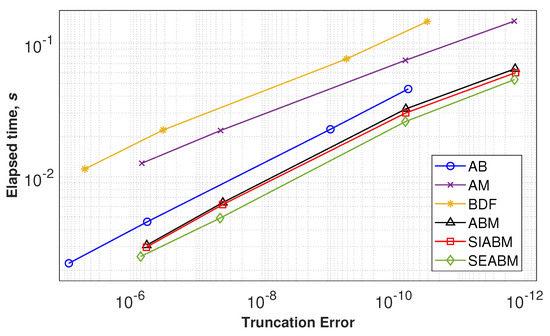
Figure 1.
Performance plots for compared multistep ordinary differential equation (ODE) solvers while simulating system (6) with fixed step.
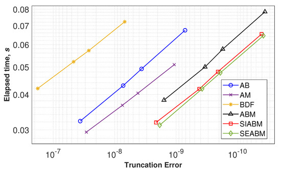
Figure 2.
Performance plots for compared multistep ODE solvers when simulating system (6) with variable step.
Figure 2 represents the results of performance analysis for studied solvers with the variable stepsize. It is known that for multistep integration methods step-size control supposes more computational costs than for single-step solvers. In our study, we implemented methods with an uneven grid, for which the recursive calculation of the method coefficients is required when the integration step value is changed [1]. As one can see, this leads to a reduction of the difference in the computational costs between explicit and implicit algorithms (Figure 2). The proposed SIABM and SEABM solvers possess a higher speed of computation with similar accuracy being compared with the known ABM technique.
3.2. Rossler Chaotic System
As the second sample system, the Rossler oscillator [22] was chosen. This system is described by the following ODEs
where are free parameters. We investigated system (7) with , which correspond to the case of chaotic oscillations [22].
System (7) was simulated with variable and fixed integration step for time s from initial conditions by all compared methods. Figure 3 and Figure 4 represent the results of this experiment. As one can see, in the case of the three-dimensional system, superiority in the performance of fixed-step solvers based on the proposed methods over the conventional ABM scheme is more noticeable. The accuracy of the solutions calculated by semi-explicit and semi-implicit techniques is comparable with the results obtained for the implicit AM method. All of the predictor-corrector methods appear to be the most efficient among the considered integration schemes.
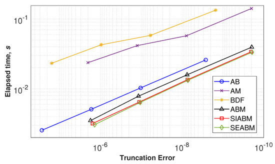
Figure 3.
Performance plots for investigated multistep ODE solvers simulating system (7) with fixed step.
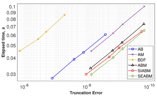
Figure 4.
Performance plots for investigated multistep ODE solvers simulating system (7) with variable step.
Step-size control reinforces the difference in the performance of ODE solvers based on predictor-corrector schemes in comparison with the explicit AB method (Figure 4). Moreover, the explicit AB algorithm shows a significant decrease in accuracy when the system with chaotic behavior is simulated. The most effective method is the semi-explicit technique, as was in the case of the van der Pol oscillator.
Thus, we can conclude that semi-implicit and semi-implicit multistep integration for both considered systems are more efficient when implemented with the variable step.
4. Discussion
The computational costs of the proposed semi-implicit solver can increase significantly if Newton’s iterations will be required for approximation of diagonally implicit variable. Figure 5 shows the simulation results for the Rossler system using proposed four-stage ODE solvers with various approximation techniques for diagonal implicitness. We compared the SEAM algorithm with methods which involve Newton’s iterations (SIABMN) and simple iterations (SIABMSI) as well as the SIABM method with the analytical solution of diagonally implicit algebraic equations. To clarify the comparison and increase the understandability we provide listings of the used algorithms in Appendix A, excluding code for the (SIABMN) method due to its massiveness. As one can see from Figure 5, the semi-implicit ABM modification with the Newton method is the most computationally expensive solver. This method should be applied only if it is impossible to resolve a system of diagonally implicit algebraic equations. The examples of such systems can be the simple model of spiking neurons [23] and the Hodgkin-Huxley system [24] which are broadly used in computational neuroscience. An alternative to Newton’s method is the simple iterations algorithm (SIABMSI in Figure 5), which is less computationally expensive and is proven to be convergent for arbitrary right-hand side function [16].
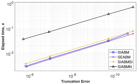
Figure 5.
Performance plots for various semi-implicit and semi-explicit multistep ODE solvers simulating system (7) with fixed step.
One can note that the semi-explicit integration is free from this limitation but potentially possesses less stability and convergence, especially for high-dimensional systems.
5. Conclusions
In this study we proposed the simple technique to enhance the performance of predictor-corrector multistep ODE solvers. We described two versions of the modified Adams-Bashforth-Moulton method with semi-implicit and semi-explicit integration. The proposed numerical integration methods possess high precision and low computational costs. In the experimental part of the study, we have explicitly shown that the performance of semi-implicit and semi-explicit multistep integration methods is superior to their explicit and implicit counterparts. To illustrate this, we simulated two nonlinear systems: the van der Pol oscillator and the chaotic Rossler system. In both cases, the computational efficiency of semi-explicit and semi-implicit Adams-Bashforth-Moulton methods was highest among the tested algorithms. Implementation with adaptive stepsize confirmed this property of proposed methods. In our further research, we will compare these algorithms with high-order single-step solvers, including semi-explicit and semi-implicit extrapolation and composition methods, as well as the effects arising in the long-term simulation of nonlinear systems.
Author Contributions
Conceptualization, D.B.; data curation, A.T. and T.K.; formal analysis, A.T. and D.B.; funding acquisition, D.B.; investigation, A.T.; methodology, D.B.; project administration, D.B.; resources, T.K.; software, A.T. and T.K.; supervision, D.B.; validation, D.B.; visualization, T.K.; writing—original draft, A.T. and D.B.; writing—review & editing, A.T., T.K. and D.B. All authors have read and agreed to the published version of the manuscript.
Funding
Denis Butusov was funded by the grant of the Russian Science Foundation (RSF), project 19-71-00087.
Conflicts of Interest
The authors declare no conflict of interest.
Appendix A. Pseudocodes of the Proposed Methods for the Simulation of Rossler System
List of used notations:
- state variables at the time moment i:
- parameter values:
- coefficients of the four-stage Adams-Bashforth method:
- coefficients of the four-stage Adams-Moulton method:
- value of the right-hand side function for variable j at the time moment i obtained from the previous iterations:
- integration step: h
| Listing A1. Single integration step for the semi-explicit Adams-Bashforth-Moulton method |
| #Predictor |
| #Corrector |
| Listing A2. Single integration step for the semi-implicit Adams-Bashforth-Moulton method. In this case the analytic solution of the diagonally implicit algebraic equations is derived. |
| #Predictor |
| #Corrector |
| #Solving algebraic equation with respect to |
| #Solving algebraic equation with respect to |
| Listing A3. Single integration step for the semi-implicit Adams-Bashforth-Moulton method. Case with the simple iterations. |
| #Predictor |
| #Corrector |
| #First simple iteration for |
| #Second simple iteration for |
| #First simple iteration for |
| #Second simple iteration for |
References
- Hairer, E.; Nørsett, S.P.; Wanner, G. Solving Ordinary Differential Equations I: Nonstiff Problems; Springer: Berlin, Germany, 1993; Volume 8. [Google Scholar] [CrossRef]
- Mohd Ijam, H.; Ibrahim, Z.B. Diagonally Implicit Block Backward Differentiation Formula with Optimal Stability Properties for Stiff Ordinary Differential Equations. Symmetry 2019, 11, 1342. [Google Scholar] [CrossRef]
- Jana Aksah, S.; Ibrahim, Z.B.; Zawawi, M.; Shah, I. Stability analysis of singly diagonally implicit block backward differentiation formulas for stiff ordinary differential equations. Mathematics 2019, 7, 211. [Google Scholar] [CrossRef]
- Feng, K.; Qin, M. Symplectic Geometric Algorithms for Hamiltonian Systems; Springer: Berlin, Germany, 2010. [Google Scholar]
- Iavernaro, F.; Mazzia, F.; Mukhametzhanov, M.; Sergeyev, Y.D. Conjugate-symplecticity properties of Euler–Maclaurin methods and their implementation on the Infinity Computer. Appl. Numer. Math. 2019, 155, 58–72. [Google Scholar] [CrossRef]
- Zhang, H.; Qian, X.; Song, S. Novel high-order energy-preserving diagonally implicit Runge–Kutta schemes for nonlinear Hamiltonian ODEs. Appl. Math. Lett. 2020, 102, 106091. [Google Scholar] [CrossRef]
- Hairer, E.; Lubich, C.; Wanner, G. Geometric numerical integration illustrated by the Störmer–Verlet method. Acta Numer. 2003, 12, 399–450. [Google Scholar] [CrossRef]
- Forest, E.; Ruth, R.D. Fourth-order symplectic integration. Phys. D Nonlinear Phenom. 1990, 43, 105–117. [Google Scholar] [CrossRef]
- Forest, E. Geometric integration for particle accelerators. J. Phys. A Math. Gen. 2006, 39, 5321. [Google Scholar] [CrossRef]
- Hairer, E.; Lubich, C.; Wanner, G. Geometric Numerical Integration: Structure-Preserving Algorithms for Ordinary Differential Equations; Springer Science & Business Media: Berlin, Germany, 2006; Volume 31. [Google Scholar] [CrossRef]
- Holder, T.; Leimkuhler, B.; Reich, S. Explicit variable step-size and time-reversible integration. Appl. Numer. Math. 2001, 39, 367–377. [Google Scholar] [CrossRef]
- Nikitin, N. Third-order-accurate semi-implicit Runge–Kutta scheme for incompressible Navier–Stokes equations. Int. J. Numer. Methods Fluids 2006, 51, 221–233. [Google Scholar] [CrossRef]
- McLachlan, R.I.; Quispel, G.R.W. Splitting methods. Acta Numer. 2002, 11, 341–434. [Google Scholar] [CrossRef]
- Butusov, D.; Tutueva, A.; Homitskaya, E. Extrapolation Semi-implicit ODE solvers with adaptive timestep. In Proceedings of the 2016 XIX IEEE International Conference on Soft Computing and Measurements (SCM), St. Petersburg, Russia, 25–27 May 2016; pp. 137–140. [Google Scholar] [CrossRef]
- Yoshida, H. Construction of higher order symplectic integrators. Phys. Lett. A 1990, 150, 262–268. [Google Scholar] [CrossRef]
- Butusov, D.N.; Ostrovskii, V.Y.; Karimov, A.I.; Andreev, V.S. Semi-explicit composition methods in memcapacitor circuit simulation. Int. J. Embed. Real-Time Commun. Syst. (IJERTCS) 2019, 10, 37–52. [Google Scholar] [CrossRef]
- Butusov, D.; Karimov, A.; Andreev, V. Computer simulation of chaotic systems with symmetric extrapolation methods. In Proceedings of the 2015 XVIII International Conference on Soft Computing and Measurements (SCM), St. Petersburg, Russia, 19–21 May 2015; pp. 78–80. [Google Scholar] [CrossRef]
- Butusov, D.; Karimov, A.; Tutueva, A. Symmetric extrapolation solvers for ordinary differential equations. In Proceedings of the 2016 IEEE NW Russia Young Researchers in Electrical and Electronic Engineering Conference (EIConRusNW), St. Petersburg, Russia, 2–3 February 2016; pp. 162–167. [Google Scholar] [CrossRef]
- Casas, F.; Escorihuela-Tomàs, A. Composition Methods for Dynamical Systems Separable into Three Parts. Mathematics 2020, 8, 533. [Google Scholar] [CrossRef]
- Press, W.H.; Teukolsky, S.A.; Vetterling, W.T.; Flannery, B.P. Numerical Recipes 3rd Edition: The Art of Scientific Computing; Cambridge University Press: Cambridge, UK, 2007. [Google Scholar]
- Nepomuceno, E.G.; Junior, H.M.R.; Martins, S.A.; Perc, M.; Slavinec, M. Interval computing periodic orbits of maps using a piecewise approach. Appl. Math. Comput. 2018, 336, 67–75. [Google Scholar] [CrossRef]
- Rössler, O.E. An equation for continuous chaos. Phys. Lett. A 1976, 57, 397–398. [Google Scholar] [CrossRef]
- Izhikevich, E.M. Simple model of spiking neurons. IEEE Trans. Neural Netw. 2003, 14, 1569–1572. [Google Scholar] [CrossRef] [PubMed]
- Hodgkin, A.L.; Huxley, A.F. A quantitative description of membrane current and its application to conduction and excitation in nerve. J. Physiol. 1952, 117, 500–544. [Google Scholar] [CrossRef] [PubMed]
© 2020 by the authors. Licensee MDPI, Basel, Switzerland. This article is an open access article distributed under the terms and conditions of the Creative Commons Attribution (CC BY) license (http://creativecommons.org/licenses/by/4.0/).