Abstract
This paper presents an evolutionary algorithm that simulates simplified scenarios of the diffusion of an infectious disease within a given population. The proposed evolutionary epidemic diffusion (EED) computational model has a limited number of variables and parameters, but is still able to simulate a variety of configurations that have a good adherence to real-world cases. The use of two space distances and the calculation of spatial 2-dimensional entropy are also examined. Several simulations demonstrate the feasibility of the EED for testing distinct social, logistic and economy risks. The performance of the system dynamics is assessed by several variables and indices. The global information is efficiently condensed and visualized by means of multidimensional scaling.
1. Introduction
The diffusion of a infectious disease within a given population during a short time period is called an epidemic. If the infection spreads to a large number of countries and to other continents it may be classified as a pandemic. Recent outbreaks are the 2003 severe acute respiratory syndrome (SARS), 2004 H5N1 (Avian flu), 2005 Zika fever, 2009 H1N1 and HIV/AIDS pandemics, just to name a few [1,2,3,4,5]. Presently the Coronavirus disease 2019 (COVID-19) is of utmost importance for the human species [6,7,8,9,10]. For controlling an outbreak, governments adopt basic containment, mitigation and suppression strategies. Containment is considered the early stages of the outbreak, for trying to stop the infection from being transmitted to the rest of the population. Mitigation is adopted to slow down the spread of the disease to moderate its effects on the population and the health care system. Suppression, attempts to reverse the pandemic by reducing the so-called basic reproduction number , to a value less than 1 [11,12].
The political and logistic management of an infectious outbreak is of key importance in order to decrease the epidemic peak, often called as ‘flattening the epidemic curve’. A second political issue is to handle the consequences in economy, with governments investing huge capitals to reduce the threats posed by the pandemics. In both cases, tools for estimating and foreseeing the evolution of the spread are an invaluable asset for decision makers. We find studies adopting a variety of approaches going from the use of models based on mathematical tools [13,14], such as systems of differential equations [15,16,17], or data fitting techniques and statistics, up to computer assisted strategies [18,19,20,21]. In the present days, artificial intelligence and soft computing are gaining importance and they lead to reliable methods to handle problems difficult to model and involving variables, either impossible to measure, or exhibiting unreliable values.
We find nowadays relevant initiatives involving political, academic and social organizations, trying to give a fast response to urgent problems based on data-driven and computational resources. For example, in the scope of the COVID-19 outbreak we can mention the daily update by the Italian Department of Civil Protection http://opendatadpc.maps.arcgis.com/apps/opsdashboard/index.html#/b0c68bce2cce478eaac82fe38d4138b1, the European Centre for Disease Prevention and Control https://www.ecdc.europa.eu/en/publications-data/download-todays-data-geographic-distribution-covid-19-cases-worldwide, the ‘Acción Matemática contra el Coronavirus’, http://matematicas.uclm.es/cemat/covid19/en/ by the Spanish Mathematics Committee, or the Global research on coronavirus disease (COVID-19) https://www.who.int/emergencies/diseases/novel-coronavirus-2019/global-research-on-novel-coronavirus-2019-ncov by the World Health Organization (WHO), just to name a few.
In this area of computer science, evolutionary computation provides a framework for optimization schemes inspired by biological evolution [22,23,24,25,26]. In general, evolutionary computation leads to a family of population-based optimization algorithms [27,28], with a numerical trial and error meta-heuristic and probabilistic behavior [29,30,31,32,33]. An initial set of elements in a population (often called candidate solutions) are generated and successively updated by means of some logical rules including some random variations. Probably the most well-known scheme is the ‘genetic algorithm’ [34], where a population is subjected to natural selection using mutation and crossover operations. The population gradually evolves to increase its performance according with a given fitness function chosen by the user.
In the last decades a large variety of Evolutionary algorithms (EA) were proposed. In 2013 Iztok Fister [35] presented a brief review of EA and found 74 algorithms that could be distributed in four classes, namely the families entitled swarm intelligence, biological inspired, or physics and chemistry based algorithms and miscellaneous schemes. A search in scientific and technical literature reveals a large number of proposed techniques for EA, demonstrating their popularity in the research community for dealing with real-world problems [36,37,38].
In the case of health care systems, machine learning algorithms have also been explored. Interested readers can find a review in Reference [39]. In what concerns specific diseases, we find, for example, the problem of distinguishing bacterial from viral meningitis through a machine learning using a data set [40]. Nonetheless, we must have in mind that in pervasive/ubiquitous computing environments, users may evaluate their trustworthiness by using historical data from their past interactions, and that some solution detecting unfair recommendations must be implemented [41].
The classical approach for compartmental models in epidemiology follows the so-called SIR model by Kermack et al. [13,42,43,44], described by a system of differential equations, where a fixed population of individuals that fit into three categories, namely the susceptible (but not yet infected), infectious and recovered (with immunity) individuals, that vary in time. The small number of variables and parameters limit its applicability and several improvements have been proposed [45,46,47]. Nonetheless, the additional degrees of freedom come at the cost of an extra complexity often requiring variables and parameters either not available in real world, or with a considerable noise and uncertainty due to a variety of factors. Therefore, we can question if a computational scheme following the concepts of EA can overcome those problems and represent a valid alternative for modeling purposes.
Having these ideas in mind, this paper develops an EA for mimicking a epidemic diffusion within a population. As usual with these computational schemes several simplifications will be adopted both to speed-up the computational processing and to clarify the role of the distinct parameters and variables. In fact, we can add extra degrees of sophistication and detail at the expense of building a logical scheme leading to results more difficult to interpret given the plethora of cross effects. In spite of the simplification, we shall have a considerable number of variables and scenarios which makes difficult to compare the results. In order to overcome this problem, we adopt the multidimensional scaling (MDS) technique [48,49,50,51]. The MDS is a data processing numerical technique that allows depicting in a low dimensional locus results from a high-dimensional space. This strategy leads to a computational visualization that unravels the most important aspects embedded in the data.
The paper is organized as follows. Section 2 discusses the main ideas and formulates the structure of the proposed evolutionary epidemic diffusion (EED). Section 3 and Section 4 discuss the results given by the EED and explore several possible configurations of the parameters and distinct scenarios. Section 5 analyses the results by means MDS. Finally, Section 6 summarizes the main conclusions.
2. The Evolutionary Epidemic Diffusion Algorithm
The EED adopts a 2-dimensional squared small-world (SW) with a population of N elements, so that the i-th individual is positioned on the coordinates , , inside the square. The population will evolve in time t and in the 2-dimensional space according with the rules defined in the sequel. Two exceptions outside the coordinates of the SW are considered consisting of the ‘hospital and house’ (hereafter simply denoted as hospital) and ‘cemetery’. These two additional repositories are allocated to the elements of the population that are found by health care system as infected or that passed away due to the action of the virus. The population is distributed along five categories: ‘healthy’, ‘infected’ (but not in hospital or confined in house) and ‘immunized’ that move in time and space, the ‘hospitalized’ corresponding to infected people that are taken to the hospital or that are confined to some part of his house in case the health state is not too serious, and ‘dead’ that are positioned in the ‘cemetery’.
The population is initialized in 2 categories ‘healthy’ and ‘infected’ with percentages and , respectively. Let us suppose that two individuals in the SW can be randomly selected. If they are in a distance range inferior to a given threshold limit, that may be called ‘social neighborhood’, D, and if one is healthy and the other is infected, then the healthy became infected with a probability , otherwise he stays in the previous state. Therefore, if and are the coordinates of the i-th and j-th individuals () and one is infected, then infection of the other will occur with probability if , where the spatial distance d is defined as [52]:
An infected individual can remain as ‘infected’ with probability if not detected by the health care system (either due to logistic limitations, or because of being asymptomatic). Nonetheless, an ‘infected’ individual can change to the categories ‘hospitalized’, ‘dead’, or ‘immunized’ as described in the follow-up. The hospital has limited capacity of places. Therefore, an infected individual that is detected by the health care system, can enter in the hospital if, and only if, the number of patients does not surpass the limit, that is . Moreover, infected and hospitalized individuals can change to the category ‘dead’ with probabilities and , respectively. The infected or hospitalized i-th individual changes to ‘immunized’ after being in that state for the period of time , where stands for some random variation with a uniform probability distribution. Individuals ‘immunized’ re-enter the SW with randomly generated coordinates and cannot be infected again. Moreover, dead or immunized do not transmit infection to others.
The population located in the SW (i.e., ‘healthy’, ‘infected’ and ‘immunized’) changes position in space with a small increment generated randomly and independently with uniform distribution and zero mean. Therefore, the ith individual evolves in space between two successive time iterations t and . In the follow-up, we consider that the maximum displacement values are identical (i.e., ). Therefore, two independent values and are generated, as long as the new coordinates remain in the SW, otherwise a new set of random displacements is generated.
The Minkowski distance d leads to the Manhattan (or city), Euclidean and Chebyshev distances [53] for . In particular, we can simulate different environments in the SW, such with and without buildings for and , respectively.
Several issues must be considered:
- The SW is considered to have an isotropic structure, that is, without a special architectural or geophysical structure. Therefore, the choice for seems intuitive.
- The uniform probability distribution is often adopted in the scope of EA, merely for the sake of simplification. The adoption of other distributions, such as the Gaussian, or the use of conditional probabilities, for example, would imply further assumptions that imply adding an extra complexity to the EED. Section 4 will discuss further this preliminary assumption.
- The Manhattan and Euclidean attempt to model distinct behaviors of the individuals moving in the SW, but not the propagation of the virus. In fact, individuals have a macroscopic nature in opposition to virus that has a microscopic dimension and can propagate in a variety of ways, such as in air by the wind or in the clothes and shoes of the host individuals. So, the city distance reflects the adoption of social attitudes such as passing for the other side of the street when another individual appears in the same direction.
In summary, the EA (i) starts with two categories ‘healthy’ and ‘infected’, (ii) evolves in time and space with five categories ‘healthy’, ‘infected’, ‘hospitalized’, ‘immunized’ and ‘dead’, and (iii) at the end the SW includes only three categories, specifically the ‘healthy’, ‘immunized’ and ‘dead’. Obviously, during the simulation the number of active individuals in the SW (i.e., those that are not ‘hospitalized’, or ‘dead’) decreases.
The overall description and assignment of variables and parameters is represented in the diagram of Figure 1.
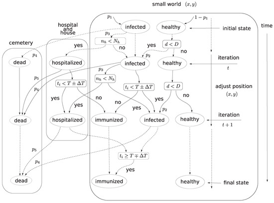
Figure 1.
Diagram of the evolutionary epidemic diffusion (EED) involving the five state variables ‘healthy’, ‘infected’, ‘hospitalized’, ‘immunized’ and ‘dead’ and the three locations small world (SW), hospital and cemetery.
Some of the simplifications may be a matter of criticism, such as:
- A 2-dimensional SW with fixed Cartesian boundaries is considered
- The SW has a uniform structure, without including rivers, hills or other structures
- The rules of the EA are fixed in time
- Some additional modeling of the hospital, such as staff burnout or equipment limitation, is absent
- The effect of different clinical conditions and age are identical for all population
- The total population decreases along time since no births or incoming visitors are included
- Hospitalized individuals can infect others, but no such case is considered
- No ‘dead’ individuals due to other causes
Indeed we can include extra rules and answer these issues. However, we must have in mind that EA are usually a simplification of the real-world. This allows a faster calculation and a simpler and more assertive interpretation of the meaning of each parameter.
3. Exploring the Evolutionary Algorithm: A First Set of Experiments
Let us consider a population of individuals with and for infected and healthy, respectively, and simulate the SW during iterations. Therefore, the EED simulation starts with ‘infected’ and ‘healthy’ individuals. The SW is delimited by the coordinates and , the infection distance is set to , and the maximum step in space between two consecutive time iterations is . Other parameters are set to , , and . The infection incubation period is set to days with a variation days, and the hospital capacity is considered unlimited. We consider low values for the mortality, such as the common flu or the COVID19, but not others such as Ebola or Marburg [2,4]. Nonetheless, the adoption of such numerical values does not precludes the use of higher values for such probabilities. Moreover, it is considered to describe the positive influence of the medical health care. Figure 2 shows the time evolution of the 5 state variables during the period of iterations for this first scenario .
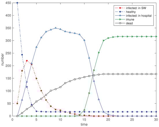
Figure 2.
Scenario : Time evolution of the 5 state variables, for , , , , , , , , , and .
We verify a fast decrease of the number of ‘hospitalized’ and an increase in the ‘immunized’. The number of ‘infected’ (not in hospital) has a slow but continuous reduction and the ‘dead’ increase linearly until the ‘immunized’ reach the steady-state. Varying the value of T changes the delay period for starting the emergence of the variable ‘immunized’. On the other hand, the main effect of increasing is to smooth the curve at the start and end of the immunization transient.
The value of represents a free space. Therefore, we consider a second scenario of a SW described by a distance with , while the rest of the parameters remain identical. Figure 3 depicts the time evolution of the 5 state variables. Comparing the two scenarios we conclude that for we have a larger number of ‘healthy’ and a smaller value for the ‘dead’.
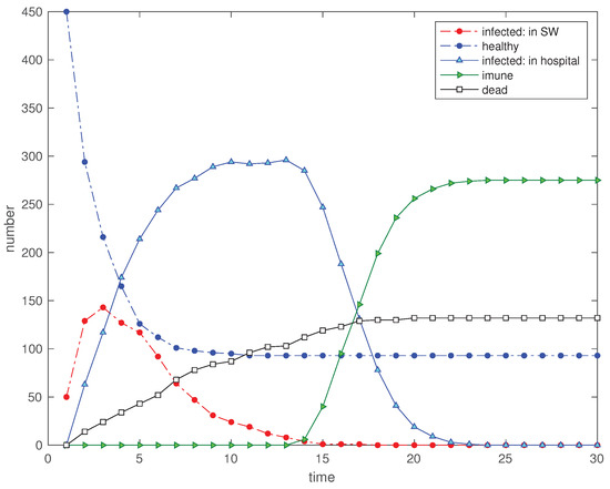
Figure 3.
Scenario : Time evolution of the 5 state variables for (, , , , , , , , and ).
In a third scenario we limit the hospital capacity (and house confinement capacity) to , that is, to 20% of the total population. The other parameters remain identical to first scenario. Figure 4 shows clearly the effect of saturation in the ‘hospitalized’ time evolution and a clear increase in the final number of ‘dead’.
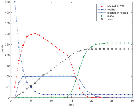
Figure 4.
Scenario : Time evolution of the 5 state variables for (, , , , , , , , and ).
In a 4th scenario we evaluate the influence of confining the individuals by reducing the distance threshold limit to while the rest of the parameters remain identical to scenario . Figure 5 shows the strong effect of the limitation that leads to the increasing of ‘healthy’, and the diminishing of ‘immunized’ and ‘dead’.
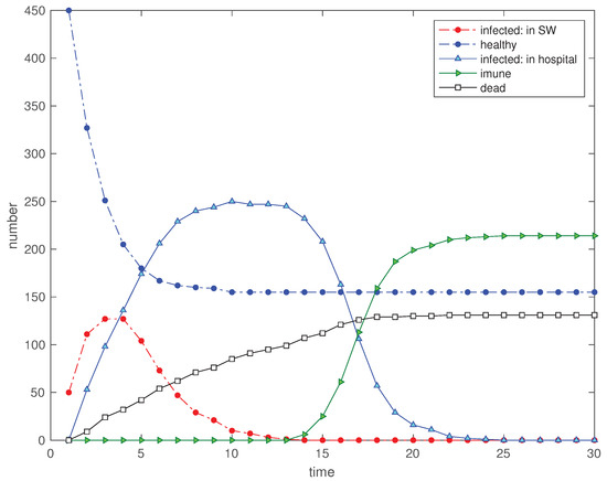
Figure 5.
Scenario : Time evolution of the 5 state variables for (, , , , , , , , and ).
Let us consider four cost indices consisting of:
- , the integral in time of the number of ‘hospitalized’ divided by the maximum value (i.e., )
- , the maximum number of ‘hospitalized’ divided by the population maximum number (i.e., N)
- , the number of ‘dead’ divided by the population maximum number (i.e., N)
- , the integral in time of the total number ‘healthy’ and ‘immunized’ divided by the maximum value (i.e., ).
The indices and assess social and logistic issues, addresses mainly a social aspect and focuses in economic matters. Table 1 lists the parameters and the obtained values of the indices for the proposed scenarios.

Table 1.
Numerical values of the EED parameters for scenarios , , and the cost indices , .
In all scenarios we find 4 phases
- starting from two categories only, namely ‘healthy’ and ‘infected’, an initial transient with a fast diminishing in the number of ‘healthy’ and an inverse behavior with the ‘infected’, ‘hospitalized’ and ‘dead’
- a slow diminishing or even a steady-state in the ‘healthy’ and a moderate increase with the ‘infected’, ‘hospitalized’ and ‘dead’
- a fast increase of the ‘immunized’ and slow decrease of ‘infected’, ‘hospitalized’ and ‘dead’,
- a steady-state with individuals in there categories only, namely ‘healthy’, ‘dead’ and ‘immunized’.
Let us now consider the influence of the control strategy based on the social neighborhood D upon the cost indices. Therefore, we simulate the EED for and we consider the effect of the social neighborhood for the cases of and . The rest of the parameters remain identical to those adopted in scenario .
Figure 6, Figure 7, Figure 8 and Figure 9 show the evolution of the four indices versus D for the two values of . In all cases we verify that the cost increases significantly for and stabilizes at an high value for . Furthermore, the value of has some influence and we verify that a SW with limits slightly the propagation of the infection in relation with the case of a SW with .
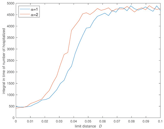
Figure 6.
Variation of the integral in time of the number of hospitalized () versus the social neighborhood D for (, , , , , , , and ).
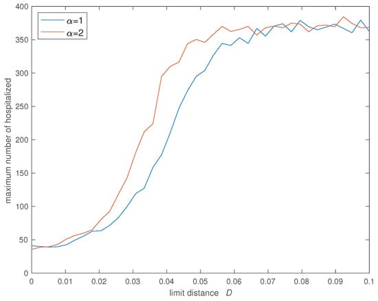
Figure 7.
Variation of the maximum number of hospitalized () versus the social neighborhood D for (, , , , , , , and ).
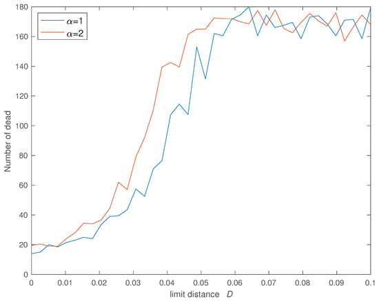
Figure 8.
Variation of the number of dead () versus the social neighborhood D for (, , , , , , , and ).
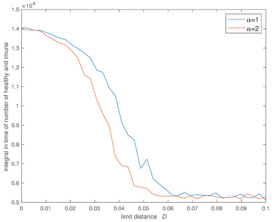
Figure 9.
Variation of the integral in time of the number of healthy and ‘immunized’ () versus the social neighborhood D for (, , , , , , , and ).
The spatial distribution of the elements in the SW can also be measured. Let us adopt the Shannon entropy of the space occupation by any type of individual, that is, ‘healthy’, ‘infected’ and ‘immunized’, since the ‘hospitalized’ and and ‘dead’ are located outside the SW namely at the ‘hospital’ and ‘cemetery’, respectively. The SW is subdivided into an array of matrix and the number of individuals in each cell in counted for obtaining a 2-dimensional histogram. The statistics of the spatial distribution versus time t is obtained my means of the 2-dimensional space entropy given by [54,55,56,57,58]:
where is the probability obtained for the -cell of the matrix, at a given time instant t.
Figure 10 illustrates the evolution of the individuals in the SW for and Figure 11 depicts the evolution of versus time t, for and . In all cases it is considered , , , , , , and . We observe clearly (i) the diminishing of the ‘healthy’ and the increase of the ‘infected’ when passing from to , (ii) the disappearance to the ‘infected’ and the emergence of the ‘immunized’ when going to and (iii) the steady-state at with ‘healthy’ and ‘immunized’. The space entropy reflects also clearly the transient and the difference between the initial condition and the steady-state.
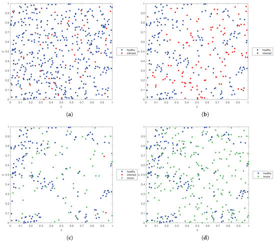
Figure 10.
State of the SW space occupation by ‘healthy’, ‘infected’ and ‘immunized’ individuals for: (a) , (b) , (c) , (d) (, , , , , , , , , and ).
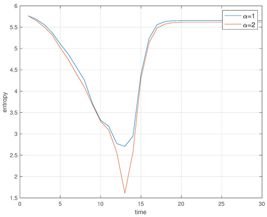
Figure 11.
Space entropy versus time t, for and (, , , , , , , , and ).
4. Exploring the Evolutionary Algorithm: A Second Set of Experiments
In the previous scenarios no available vaccine or treatment is considered. Therefore, the ‘immunized’ variable is an important issue against any new surge of infection. To illustrate this problem let us consider the 5th and 6th scenarios, and , with a disturbance of 50 recently ‘infected’ visitors entering in the SW at with coordinates generated randomly. Scenarios and follow the conditions of scenarios and (i.e., and ), respectively, for the rest of the parameters, with exception of the simulation period that is extended to .
Figure 12 and Figure 13 show the immediate effect in all variables. However, in scenario the number of ‘immunized’ is lower at and, consequently, the propagation of the perturbation is much superior.
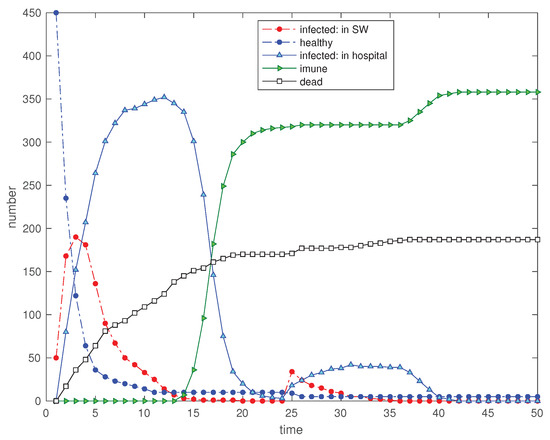
Figure 12.
Scenario : Time evolution of the 5 state variables for and a disturbance in the SW with the input of 50 new ‘infected’ visitors at (, at , , , , , , , and ).
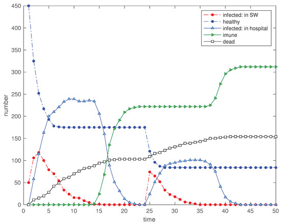
Figure 13.
Scenario : Time evolution of the 5 state variables for and a disturbance in the SW with the input of 50 new ‘infected’ visitors at (, at , , , , , , , and ).
The public feeling of risk as a consequence of known critical cases is a variable that we can consider and implement in the EED. Therefore, we consider a scenario where a disturbance is simulated by reducing the social neighborhood to for . Figure 14 shows clearly the reduction of ‘hospitalized’, ‘dead’ and ‘immunized’ and, correspondingly, the improvement in the cost functions.
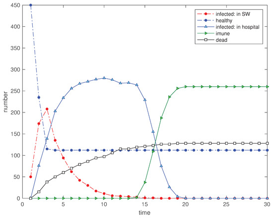
Figure 14.
Scenario : Time evolution of the 5 state variables for a disturbance in the SW so that for , and for (, , , , , , , , and ).
During the outbreak of the virus spread some medical drug for an efficient treatment may be discovered and administrated to all population, both hospitalized and non-hospitalized. To simulate this scenario we consider a disturbance at , where the probabilities of death are set to the values . Figure 15 shows again a remarkable improvement.
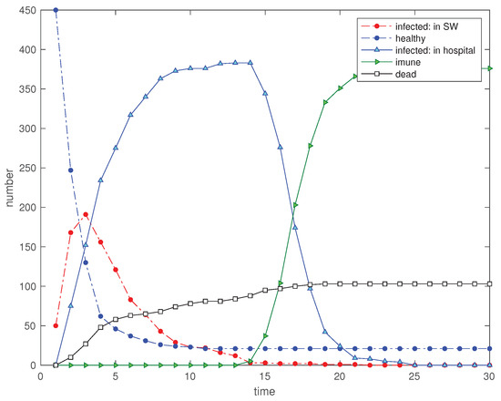
Figure 15.
Scenario : Time evolution of the 5 state variables for a disturbance in the SW so that and for , and and for (, , , , , , and ).
Another issue to consider is the initialization of the EED. In the scenarios adopted so far, the simulation starts with a considerable number of ‘infected’, namely with 50 individuals in a total of 500. To evaluate the effect of starting with a smaller number, we consider 5, 10 and 20 ‘infected’ (see Figure 16, Figure 17 and Figure 18) corresponding to the scenarios , and , respectively. We verify clearly a smother variation of the curves and the improvement in the cost indices, demonstrating the importance of an early detection of the ‘infected’.
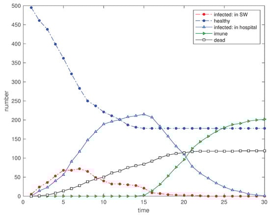
Figure 16.
Scenario : Time evolution of the 5 state variables for (, , , , , , and ).
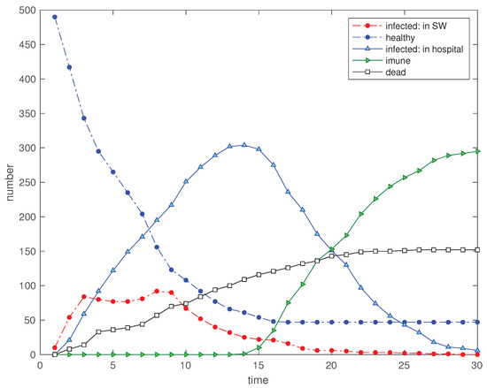
Figure 17.
Scenario : Time evolution of the 5 state variables for (, , , , , , and ).
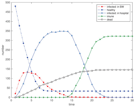
Figure 18.
Scenario : Time evolution of the 5 state variables for (, , , , , , and ).
Table 2 lists the parameters and the obtained values of the indices for the seven new scenarios.
Table 2.
Numerical values of the EED parameters for scenarios , , and the cost indices , .
5. Multidimensional Scaling Analysis of the Evolutionary Algorithm
The results given by the EED have a probabilistic nature and vary slightly in each run. Moreover, we have a large number of variables which makes difficult to compare the results. In order to overcome these problems we adopt the multidimensional scaling (MDS) technique [48,49,50,51] to condense the results in a single representation. In short, the MDS represents in a low dimensional space (i.e., with dimension q) data sets from an higher dimensional space (i.e., with dimension ), while preserving its main characteristics and highlighting the key issues. For achieving that goal the MDS computational algorithms requires two phases. In a first phase the user defines a given distance d comparing the set of items in a p-dimensional space [52,53]. Then, all items are compared by calculating a matrix , , with and , of item-to-item distances in the p-dimensional space. In a second phase, the MDS performs successive iterations trying to find a configuration of items in the q-dimensional space that mimic approximately the original distances. Usually the MDS adopts a numerical strategy for minimizing some kind of least squares index, often called stress. Several distinct types of distances can be used. Also, since we are dealing with relative measurements (i.e., distances), the representation in the q-dimensional space is read in terms of clusters and can be rotated, magnified or shifted since the axis have no physical interpretation. Often the dimensions or are adopted since they allow a straightforward visualization [59,60,61].
We consider data sets produced by the EED with vectors , and , for the five variables and time of simulation, respectively. For calculating the distances between items we adopt the Canberra and Lorentzian metrics, and , to assess the dissimilarity between pairs:
where and denote two time instants, so that . Therefore, in this case the matrices have dimension , for both distances.
Additionally, we consider 10 runs to evaluate the probabilistic effect and 3 scenarios for the social neighborhood . We overlap the 10 MDS loci using the Procrustes technique [62,63]. The Procrustes processing between two matrices and of identical dimension determines a linear transformation (i.e., a translation, reflection, orthogonal rotation, and scaling) of the points in matrix to best conform them to the points in matrix .
Figure 19 and Figure 20 show the resulting MDS loci for and the Canberra (3) and Lorentzian (4) distances, respectively. The numerical parameters are , , , , , , , and . The initial time instants, corresponding to , are marked with small circles.
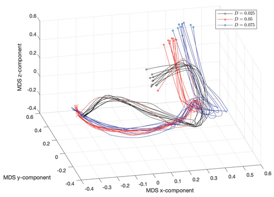
Figure 19.
The 3-dimensional multidimensional scaling (MDS) locus, using the Canberra distance (3), , for (, , , , , , , and ).
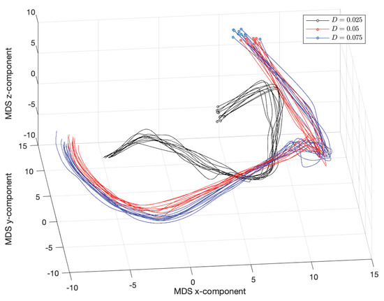
Figure 20.
The 3-dimensional MDS locus, using the Lorentzian distance (4), , for (, , , , , , , and ).
We verify clearly the emergence of the phase , , observed in the first group of experiments. Nonetheless, as usual with MDS, the two distances capture slightly distinct aspects of the time series in what concerns the three distinct scenarios for D. The Canberra distance highlights the distinct initial transients, while the crossover instants ( and ) between phases and the steady state have close characteristics. On the other hand, the Lorentzian distance considers that the three scenarios have similar topological form, having merely a distinct scale factor.
We test also the EED for the collection of scenarios , , corresponding to the combination of three values of the social neighborhood and three values of the hospital capacity . The average of the cost indices , , for 10 independent runs of each scenario, are listed in Table 3. We can also use the MDS to visualize the information using the Canberra and Lorentzian metrics, and , that in this case are written as:
where the vectors , , and , include the values of the 4 cost indices for the nine scenarios with 10 runs each. Therefore, in this case each matrix has dimension .
Table 3.
Numerical values of the EED parameters for scenarios , , and the average of the cost indices , , for 10 independent runs.
Figure 21 and Figure 22 show the MDS loci for and the Canberra (5) and Lorentzian (6), respectively. The loci reveal clearly that the pairs of scenarios , and have some similarities. On the other hand, the scenarios , and have, each one, a very distinct behavior. These results show that the combination of the parameters D and are of utmost importance.
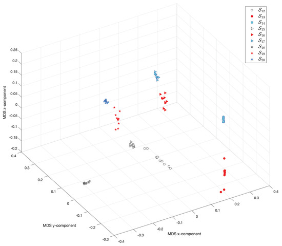
Figure 21.
The 3-dimensional MDS locus, using the Canberra distance (5), for 10 runs of each scenario , , with performance captured by the cost indices , .
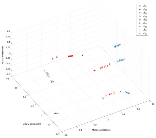
Figure 22.
The 3-dimensional MDS locus, using the Lorentzian distance (6), for 10 runs of each scenario , , with performance captured by the cost indices , .
6. Conclusions
This paper presented an EA that simulates the propagation of a virus infection in a SW. The EED includes a limited number of variables and parameters, but characterizes a large number of possible scenarios and allows a fast computational simulation. In fact, the extension of the EED to include additional factors present in the real world is reasonably straightforward, but the limitation of the EED complexity follows the usual strategy of developing EA with focus on the most important variables and parameters. Several scenarios were tested and the results follow the common intuition about the diffusion of infectious diseases. The system, involving several variables and parameters, was assessed by several tools and performance indices. The MDS technique proved to be a valuable tool to condense the multidimensional nature of the information. In fact, this technique takes also advantage of present day computational resources and allows unraveling patterns embedded in complex data and tracing conclusions that otherwise would require laborious schemes to highlight the main conclusions. In summary, the EED represents a valuable computational tool for the development of strategies for simulating, controlling and foreseeing future results of virus outbreaks.
Funding
This research received no external funding.
Conflicts of Interest
The author declares no conflict of interest.
References
- Cox, C.M.; Blanton, L.; Dhara, R.; Brammer, L.; Finelli, L. 2009 Pandemic Influenza A (H1N1) Deaths among Children—United States, 2009–2010. Clin. Infect. Dis. 2011, 52, S69–S74. [Google Scholar] [CrossRef]
- Lopes, A.M.; Andrade, J.P.; Machado, J.T. Multidimensional scaling analysis of virus diseases. Comput. Methods Programs Biomed. 2016, 131, 97–110. [Google Scholar] [CrossRef]
- Kibona, I.; Yang, C. SIR Model of Spread of Zika Virus Infections: ZIKV Linked to Microcephaly Simulations. Health 2017, 9, 1190–1210. [Google Scholar] [CrossRef][Green Version]
- Lopes, A.M.; Machado, J.A.T.; Galhano, A.M. Computational Comparison and Visualization of Viruses in the Perspective of Clinical Information. Interdiscip. Sci. Comput. Life Sci. 2017, 11, 86–94. [Google Scholar] [CrossRef]
- Yu, P.; Zhang, W. Complex Dynamics in a Unified SIR and HIV Disease Model: A Bifurcation Theory Approach. J. Nonlinear Sci. 2019, 29, 2447–2500. [Google Scholar] [CrossRef]
- Zhu, N.; Zhang, D.; Wang, W.; Li, X.; Yang, B.; Song, J.; Zhao, X.; Huang, B.; Shi, W.; Lu, R.; et al. A Novel Coronavirus from Patients with Pneumonia in China, 2019. N. Engl. J. Med. 2020, 382, 727–733. [Google Scholar] [CrossRef]
- Chinazzi, M.; Davis, J.T.; Ajelli, M.; Gioannini, C.; Litvinova, M.; Merler, S.; y Piontti, A.P.; Mu, K.; Rossi, L.; Sun, K.; et al. The effect of travel restrictions on the spread of the 2019 novel coronavirus (COVID-19) outbreak. Science 2020, 368, 395–400. [Google Scholar] [CrossRef]
- Li, C.; Yang, Y.; Ren, L. Genetic evolution analysis of 2019 novel coronavirus and coronavirus from other species. Infect. Genet. Evol. 2020, 82, 104285. [Google Scholar] [CrossRef]
- Chen, S.; Yang, J.; Yang, W.; Wang, C.; Bärnighausen, T. COVID-19 control in China during mass population movements at New Year. Lancet 2020, 395, 764–766. [Google Scholar] [CrossRef]
- Kissler, S.M.; Tedijanto, C.; Goldstein, E.; Grad, Y.H.; Lipsitch, M. Projecting the transmission dynamics of SARS-CoV-2 through the postpandemic period. Science 2020, 368, eabb5793. [Google Scholar] [CrossRef]
- Jones, J.H. Notes on 0; Technical Report; Stanford University: Stanford, CA, USA, 2007. [Google Scholar]
- Fraser, C.; Donnelly, C.A.; Cauchemez, S.; Hanage, W.P.; Kerkhove, M.D.V.; Hollingsworth, T.D.; Griffin, J.; Baggaley, R.F.; Jenkins, H.E.; Lyons, E.J.; et al. Pandemic Potential of a Strain of Influenza A (H1N1): Early Findings. Science 2009, 324, 1557–1561. [Google Scholar] [CrossRef]
- Kermack, W.O.; McKendrick, A.G. A contribution to the mathematical theory of epidemics. Proc. R. Soc. Lond. Ser. A Contain. Pap. A Math. Phys. Character 1927, 115, 700–721. [Google Scholar] [CrossRef]
- Kucharski, A.J.; Russell, T.W.; Diamond, C.; Liu, Y.; Edmunds, J.; Funk, S.; Eggo, R.M.; Sun, F.; Jit, M.; Munday, J.D.; et al. Early dynamics of transmission and control of COVID-19: A mathematical modelling study. Lancet Infect. Dis. 2020, 20, 553–558. [Google Scholar] [CrossRef]
- Grenfell, B.T.; Bjørnstad, O.N.; Finkenstädt, B.F. Dynamics of Measles Epidemics: Scaling Noise, Determinism, and Predictability with the TSIR Model. Ecol. Monogr. 2002, 72, 185–202. [Google Scholar] [CrossRef]
- Huang, Z.; Yang, Q.; Cao, J. Complex dynamics in a stochastic internal HIV model. Chaos Solitons Fractals 2011, 44, 954–963. [Google Scholar] [CrossRef]
- Hassouna, M.; Ouhadan, A.; Kinani, E.E. On the solution of fractional order SIS epidemic model. Chaos Solitons Fractals 2018, 117, 168–174. [Google Scholar] [CrossRef]
- Kao, P.; Yang, R. Virus diffusion in isolation rooms. J. Hosp. Infect. 2006, 62, 338–345. [Google Scholar] [CrossRef]
- Balcan, D.; Gonçalves, B.; Hu, H.; Ramasco, J.J.; Colizza, V.; Vespignani, A. Modeling the spatial spread of infectious diseases: The GLobal Epidemic and Mobility computational model. J. Comput. Sci. 2010, 1, 132–145. [Google Scholar] [CrossRef]
- Immonen, T.; Gibson, R.; Leitner, T.; Miller, M.A.; Arts, E.J.; Somersalo, E.; Calvetti, D. A hybrid stochastic–deterministic computational model accurately describes spatial dynamics and virus diffusion in HIV-1 growth competition assay. J. Theor. Biol. 2012, 312, 120–132. [Google Scholar] [CrossRef]
- Britt, B.C. Modeling viral diffusion using quantum computational network simulation. Quantum Eng. 2020, 2, e29. [Google Scholar] [CrossRef]
- Goldberg, D.E. Genetic Algorithms in Search Optimization, and Machine Learning; Addison-Wesley: Reading, MA, USA, 1989. [Google Scholar]
- Koza, J.R. Genetic Programming: On the Programming of Computers by Means of Natural Selection; MIT Press: Cambridge, MA, USA, 1992. [Google Scholar]
- Michalewicz, Z. Genetic Algorithms + Data Structures = Evolution Programs; Springer: Berlin, Germany, 1996. [Google Scholar]
- Bäck, T.; Hammel, U.; Schwefel, H.P. Evolutionary computation: Comments on the history and current state. IEEE Trans. Evol. Comput. 1997, 1, 3–17. [Google Scholar] [CrossRef]
- Ashlock, D. Evolutionary Computation for Modeling and Optimization; Springer: New York, NY, USA, 2006. [Google Scholar]
- Jensen, H.J. Self-Organized Criticality: Emergent Complex Behavior in Physical and Biological System; Cambridge University Press: New York, NY, USA, 1998. [Google Scholar]
- Simon, D. Evolutionary Optimization Algorithms; Wiley: Hoboken, NJ, USA, 2013. [Google Scholar]
- Machado, J.A.T. Optimal tuning of fractional controllers using genetic algorithms. Nonlinear Dyn. 2010, 62, 447–452. [Google Scholar] [CrossRef]
- Pires, E.J.S.; Machado, J.A.T.; de Moura Oliveira, P.B.; Cunha, J.B.; Mendes, L. Particle swarm optimization with fractional-order velocity. Nonlinear Dyn. 2010, 61, 295–301. [Google Scholar] [CrossRef]
- Machado, J.T. Complex evolution of a multi-particle system. Appl. Math. Model. 2013, 37, 9203–9214. [Google Scholar] [CrossRef]
- Pires, E.J.S.; Machado, J.A.T.; de Moura Oliveira, P.B. Dynamic Shannon Performance in a Multiobjective Particle Swarm Optimization. Entropy 2019, 21, 827. [Google Scholar] [CrossRef]
- Jansen, T. Analyzing Evolutionary Algorithms: The Computer Science Perspective; Springer: Berlin/Heidelberg, Germany, 2013. [Google Scholar]
- Holland, J.H. Adaptation in Natural and Artificial Systems; The University of Michigan Press: Ann Arbor, MI, USA, 1975. [Google Scholar]
- Fister, I.; Yang, X.S.; Brest, J.; Fister, D. A Brief Review of Nature-Inspired Algorithms for Optimization. arXiv 2013, arXiv:1307.4186. [Google Scholar]
- Brownlee, J. Clever Algorithms: Nature-Inspired Programming Recipes; lulu.com: Morrisville, NC, USA, 2012. [Google Scholar]
- Câmara, D. Bio-Inspired Networking; ISTE Press: London, UK, 2015. [Google Scholar]
- Reynolds, R.G. Culture on the Edge of Chaos: Cultural Algorithms and the Foundations of Social Intelligence; Springer: Berlin/Heidelberg, Germany, 2018. [Google Scholar]
- Shailaja, K.; Seetharamulu, B.; Jabbar, M.A. Machine Learning in Healthcare: A Review. In Proceedings of the 2018 Second International Conference on Electronics, Communication and Aerospace Technology (ICECA), Coimbatore, India, 29–31 March 2018. [Google Scholar] [CrossRef]
- D’Angelo, G.; Pilla, R.; Tascini, C.; Rampone, S. A proposal for distinguishing between bacterial and viral meningitis using genetic programming and decision trees. Soft Comput. 2019, 23, 11775–11791. [Google Scholar] [CrossRef]
- D’Angelo, G.; Palmieri, F.; Rampone, S. Detecting unfair recommendations in trust-based pervasive environments. Inf. Sci. 2019, 486, 31–51. [Google Scholar] [CrossRef]
- Kermack, W.O.; McKendrick, A.G. Contributions to the mathematical theory of epidemics—I. Bull. Math. Biol. 1991, 53, 33–55. [Google Scholar] [CrossRef]
- Kermack, W.O.; McKendrick, A.G. Contributions to the mathematical theory of epidemics—II. The problem of endemicity. Bull. Math. Biol. 1991, 53, 57–87. [Google Scholar] [CrossRef]
- Kermack, W.O.; McKendrick, A.G. Contributions to the mathematical theory of epidemics—III. Further studies of the problem of endemicity. Bull. Math. Biol. 1991, 53, 89–118. [Google Scholar] [CrossRef]
- Keeling, M.J.; Rohani, P. Modeling Infectious Diseases in Humans and Animals; Princeton University Press: Princeton, NJ, USA, 2007. [Google Scholar]
- Hernandez-Vargas, E.A. Modeling and Control of Infectious Diseases in the Host: With MATLAB and R; Academic Press: San Diego, CA, USA, 2019. [Google Scholar]
- Liang, K. Mathematical model of infection kinetics and its analysis for COVID-19, SARS and MERS. Infect. Genet. Evol. 2020, 82, 104306. [Google Scholar] [CrossRef]
- Torgerson, W. Theory and Methods of Scaling; Wiley: New York, NY, USA, 1958. [Google Scholar]
- Sammon, J. A nonlinear mapping for data structure analysis. IEEE Trans. Comput. 1969, 18, 401–409. [Google Scholar] [CrossRef]
- Kruskal, J.B.; Wish, M. Multidimensional Scaling; Sage Publications: Newbury Park, CA, USA, 1978. [Google Scholar]
- Borg, I.; Groenen, P.J. Modern Multidimensional Scaling-Theory and Applications; Springer: New York, NY, USA, 2005. [Google Scholar]
- Cha, S. Taxonomy of Nominal Type Histogram Distance Measures. In Proceedings of the American Conference on Applied Mathematics, Tenerife, Spain, 15–17 December 2008; pp. 325–330. [Google Scholar]
- Deza, M.M.; Deza, E. Encyclopedia of Distances; Springer: Berlin/Heidelberg, Germany, 2009. [Google Scholar]
- Shannon, C.E. A mathematical theory of communication. Bell Syst. Tech. J. 1948, 27, 379–423, 623–656. [Google Scholar] [CrossRef]
- Jaynes, E.T. Information Theory and Statistical Mechanics. Phys. Rev. 1957, 106, 620–630. [Google Scholar] [CrossRef]
- Beck, C. Generalised information and entropy measures in physics. Contemp. Phys. 2009, 50, 495–510. [Google Scholar] [CrossRef]
- Gray, R.M. Entropy and Information Theory; Springer: New York, NY, USA, 2009. [Google Scholar]
- Machado, J.A.T. Fractional Order Generalized Information. Entropy 2014, 16, 2350–2361. [Google Scholar] [CrossRef]
- Machado, J.T. Multidimensional scaling analysis of fractional systems. Comput. Math. Appl. 2012, 64, 2966–2972. [Google Scholar] [CrossRef]
- Machado, J.A.T. Relativistic Time Effects in Financial Dynamics. Nonlinear Dyn. 2014, 75, 735–744. [Google Scholar] [CrossRef]
- Mata, M.; Machado, J. Entropy Analysis of Monetary Unions. Entropy 2017, 19, 245. [Google Scholar] [CrossRef]
- Kendall, D.G. A Survey of the Statistical Theory of Shape. Stat. Sci. 1989, 4, 87–99. [Google Scholar] [CrossRef]
- Gower, J.C.; Dijksterhuis, G.B. Procrustes Problems; OUP Oxford: Oxford, UK, 2004. [Google Scholar]
© 2020 by the author. Licensee MDPI, Basel, Switzerland. This article is an open access article distributed under the terms and conditions of the Creative Commons Attribution (CC BY) license (http://creativecommons.org/licenses/by/4.0/).