On the Selective Vehicle Routing Problem

Abstract

The Generalized Vehicle Routing Problem (GVRP) is an extension of the classical Vehicle Routing Problem (VRP), in which we are looking for an optimal set of delivery or collection routes from a given depot to a number of customers divided into predefined, mutually exclusive, and exhaustive clusters, visiting exactly one customer from each cluster and fulfilling the capacity restrictions. This paper deals with a more generic version of the GVRP, introduced recently and called Selective Vehicle Routing Problem (SVRP). This problem generalizes the GVRP in the sense that the customers are divided into clusters, but they may belong to one or more clusters. The aim of this work is to describe a novel mixed integer programming based mathematical model of the SVRP. To validate the consistency of the novel mathematical model, a comparison between the proposed model and the existing models from literature is performed, on the existing benchmark instances for SVRP and on a set of additional benchmark instances used in the case of GVRP and adapted for SVRP. The proposed model showed better results against the existing models.

1. Introduction

The Vehicle Routing Problem (VRP) is one of the most well-known and famous combinatorial optimization problems, being recorded in the literature for a long time. It was in 1959 that Dantzig and Ramser [1] first considered it when they investigated a fuel distribution problem. In this context, they provided a near optimal solution based on a linear programming formulation for the most economical collection of routes of a fleet of gasoline delivery trucks between a bulk terminal and a given number of service gas stations. There are several basic aspects that justify the significance and importance of the VRP: we can mention effective solution approaches which make it practical to solve when dealing with large graphs (see the savings algorithm developed by Clarke and Wright [2]); the problem also has numerous real-life applications in industry, especially in the areas of transportation networks and supply chain management. Finding the optimal solution to VRP is NP-hard; therefore, only problems with limited size can be solved, optimally, so a lot research is developed in the area of heuristic and metaheuristic algorithms that can provide near optimal solutions within reasonable computational times for real world VRPs.

Several variations of the VRP exist in the literature: the Capacitated Vehicle Routing Problem [3], the Vehicle Routing Problem with Pickup and Delivery [4], the Vehicle Routing Problem with Time Windows [5], the Vehicle Routing Problem with Multiple Trips [6], the Open Vehicle Routing Problem [7], the Green Vehicle Routing Problem [8], the Generalized Vehicle Routing Problem [9,10,11,12,13], the Clustered Vehicle Routing Problem [14,15,16], etc.

Recently, Posada et al. [17] considered a novel variant of the VRP, called the Selective Vehicle Routing Problem (SVRP), justified by some important real applications of the problem such as response operations in humanitarian logistics in the case of disasters where relief aid should be given to any node covering a disaster area as soon as possible, design of urban transportation routes, etc. The proposed variant extends the generalized vehicle routing problem in the sense that the nodes of the graph which are divided into clusters may belong to one or more clusters. Posada et al. [17] provided a mixed integer programming formulation of the SVRP, and in an alternative way, they have rewritten some of the constraints of the proposed model using different variants of the restrictions resulting three new mathematical formulations.

Evidently, SVRP belongs to the class of generalized combinatorial optimization problems. This category of problems naturally generalizes the classical optimization problem, having the following primary features: the vertices of the underlying graph are divided into a certain number of clusters and, when considering the feasibility constraints of the initial problem, these are expressed in relation to the clusters rather than as individual vertices. Some of the most investigated generalized combinatorial optimization problems are: the generalized minimum spanning tree problem and its variants, the generalized traveling salesman problem and its variants [18,19], the generalized vehicle routing problem and its variants [20,21], the selective graph coloring problem [22,23], the clustered shortest path tree problem, etc. For further reference on the class of generalized combinatorial optimization problems, we refer to [24,25]. A closely related problem to SVRP was introduced by Pop [18] and it was called the Selective Minimum Spanning Tree Problem. In this case, the vertices were grouped within clusters such that each vertex may belong to one ore more clusters and the objective was to find a minimum cost tree spanning a subset of vertices that includes exactly one vertex from each cluster.

The present paper is organized as follows. Section 2 provides a formal definition of the selective vehicle routing problem. Section 3 presents the novel mixed integer programming based mathematical model of the investigated problem. In Section 4, we validate the consistency of the proposed model by comparing it against the existing models from the literature on two sets of instances. The concluding results and as well as further research directions are presented.

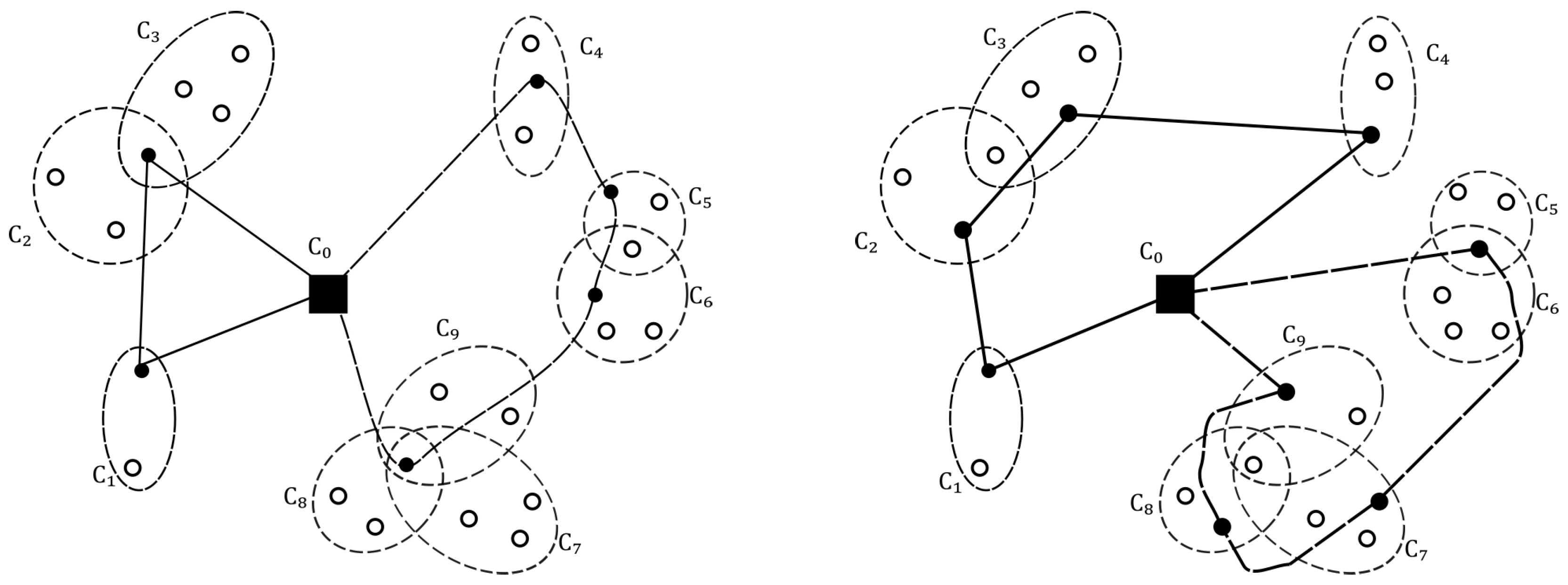
2. Definition of the Selective Vehicle Routing Problem

Let $G=\left(V,E\right)$ be an undirected graph with the set of nodes $V=\{0,1,2,\dots ,n\}$, where the node 0 represents the depot, and the set of edges $E,E\subseteq \left\{\right\{i,j\left\}\right|i,j\in V,i\ne j\}$.

The set of nodes V is divided into $m+1$ nonempty subsets denoted $C_0,C_1,\dots ,C_m$ and called clusters, where the cluster $C_0$ consists of only one node namely the depot, i.e., $C_0=\left\{0\right\}$ and the following condition holds

$$V=C_0\cup C_1\cup C_2\cup \dots \cup C_m.$$

We denote by $\mathbf{C}$ the set of all clusters and $\mathcal{C}=\left\{1,2,\dots ,m\right\}$. Dividing the nodes of the graph in this way, we do not exclude the possibility that certain nodes to belong to more than one cluster, i.e., there are $C_c,C_d\in \mathbf{C}$ such that $C_c\cap C_d\ne \varnothing$.

We associate for each node $i\in V\setminus \left\{0\right\}$ a certain demand denoted by $q_i$, $i\in \left\{1,2,\dots ,n\right\}$ and a metric coordinate denoted by $(x,y)$. Each edge $(i,j)\in E$ has associated a certain cost denoted by $d_{ij}$ and representing the Euclidean distance between the nodes i and j, with $i,j\in V$. The depot has no demand, i.e., $q_0=0$. The total demand of each cluster is obtained by summing up the demands of all the nodes belonging to that cluster and may be satisfied by any of its nodes. In addition, we assume that at the depot is based a fleet of K of identical vehicles, each with a capacity denoted by Q and $\mathcal{K}=\left\{1,2,\dots ,K\right\}$.

The goal of the Selective Vehicle Routing Problem is to determine a collection of routes, one for each vehicle, with minimum cost such that each route starts and ends at the depot, each cluster should be visited exactly once, the entering and leaving node of each cluster is the same, and the sum of all the demands of any route does not exceed the capacity of the vehicle Q. Therefore, the SVRP involves the following two related decisions:

• Select a subset of nodes $S\subseteq V$ such that $\left|S\cap C_c\right|=1$, for all $c\in \{1,\dots ,m\}=\mathcal{C}.$
• Determine a minimum cost collection of routes in the subgraph of G induced by S, satisfying the capacity constraints.

An illustrative scheme of the SVRP and two feasible collections of routes are shown in Figure 1.

In Figure 1, we present two feasible solutions of the SVRP. We can observe that the total number of visited nodes may be different: six nodes are visited in the first feasible solution and eight in the second solution. If a belonging to the three clusters $C_6,C_7$, and $C_8$ is visited, then all the nodes in the clusters $C_6,C_7$, and $C_8$ are covered.

3. A Valid Mathematical Model of Selective Vehicle Routing Problem

With the purpose of formulating the SVRP as a mixed integer linear program (MILP), we introduce the following parameters and decision variables:

• The parameter $\Lambda ={\left({\lambda }_{ic}\right)}_{\genfrac{}{}{0pt}{}{1\le i\le n}{1\le c\le m}}$ indicates if a certain node $i\in V$ belongs to a cluster $C_c$, $c\in \{1,\dots ,m\}$, thus

  $${\lambda }_{ic}=\left\{\begin{array}{c}1,\mathrm{if}i\in C_c\hfill \\ 0,\mathrm{if}i\notin C_c.\hfill \end{array}\right.$$
  This means, if the node i is an element of the cluster $C_c$, then ${\lambda }_{ic}=1$; otherwise, ${\lambda }_{ic}=0$.
• The binary decision variable $x_{ij}^k$ is defined as follows:

  $$x_{ij}^k=\left\{\begin{array}{c}1,\mathrm{if}\mathrm{the}\mathrm{vehicle}k\mathrm{traverse}\mathrm{the}\mathrm{edge}\left(i,j\right)\hfill \\ 0,\mathrm{if}\mathrm{the}\mathrm{edge}\left(i,j\right)\mathrm{is}\mathrm{not}\mathrm{part}\mathrm{of}\mathrm{any}\mathrm{route}.\hfill \end{array}\right.$$
• The integer decision variables $u_{ij}$ are defined as follows: $u_{ij}=0$ if the edge $\left(i,j\right)$ is not included in a solution route, and may take a positive integer value less or equal to n, showing its order in the corresponding route.

Then, we can express the Selective Vehicle Routing Problem as the following mixed integer programming problem:

$$\begin{array}{c}\hfill min\sum _{i=0}^n\sum _{j=0}^n\sum _{\kappa =1}^k{d}_{ij}·x_{ij}^k\end{array}$$

$$\begin{array}{c}\hfill s.t.\sum _{\genfrac{}{}{0pt}{}{i=0}{i\ne j}}^n\left(x_{ij}^k-x_{ji}^k\right)=0,\forall j\in V,k\in \mathcal{K}\end{array}$$

(1)

$$\begin{array}{c}\hfill \sum _{i=0}^n\sum _{\genfrac{}{}{0pt}{}{j=0}{i\ne j}}^n{x}_{ij}^k\ge 1,\forall k\in \mathcal{K}\end{array}$$

(2)

$$\begin{array}{c}\hfill \sum _{i=0}^n\sum _{\genfrac{}{}{0pt}{}{j=0}{i\ne j}}^n\sum _{\kappa =1}^k{\lambda }_{jc}·x_{ij}^k=1,\forall c\in \mathcal{C}\setminus \left\{0\right\}\end{array}$$

(3)

$$\begin{array}{c}\hfill \sum _{j=1}^n\sum _{k=1}^K{x}_{0j}^k=K\end{array}$$

(4)

$$\begin{array}{c}\hfill \sum _{i=0}^n\sum _{\genfrac{}{}{0pt}{}{j=0}{i\ne j}}^n{q}_i·x_{ij}^k\le Q,\forall k\in \mathcal{K}\end{array}$$

(5)

$$\begin{array}{c}\hfill n·\sum _{k=1}^K{x}_{ij}^k\ge u_{ij},\forall i,j\in V,i\ne j\end{array}$$

(6)

$$\begin{array}{c}\hfill \sum _{\genfrac{}{}{0pt}{}{j=0}{j\ne i}}^n\left(u_{ij}-u_{ji}\right)=\sum _{\genfrac{}{}{0pt}{}{j=0}{j\ne i}}^n\sum _{k=1}^K{x}_{ij}^k,\forall i\in V\end{array}$$

(7)

$$\begin{array}{c}\hfill x_{ij}^k\in \{0,1\},\forall i,j\in V,\forall k\in \mathcal{K}\end{array}$$

(8)

$$\begin{array}{c}\hfill u_{ij}\ge 0,\forall i,j\in V.\end{array}$$

(9)

Our objective is to minimize the total traveled distance. The restrictions in Equation (1) guarantee that if a vehicle reaches a certain node then it has to leave it. The restrictions in Equation (2) ensure that for every vehicle there is allocated at least one arc. The restrictions in Equation (3) guarantee that each cluster is visited exactly once. The restrictions in Equation (4) force using all the existing vehicles and in addition all the routes start and finish at the depot. The restrictions in Equation (5) provides the conditions imposed by the capacities of the vehicles. The constraints in Equations (6) and (7) are the sub-tour elimination constraints. Finally, the last constraints set the ranges of the decision variables.

4. Computational Results

To solve the proposed mathematical formulation of the SVRP, we used CPLEX 12.9. The computational experiments were performed on a PC with Procesor AMD Ryzen 9 12-Core, 64 GB RAM, Windows 10 operating system.

We report two sets of experiments: the first one compares our achieved results against the results obtained by Posada et al. [17] on a set of 36 SVRP instances generated by the same authors and the second one on a new set of instances containing 120 instances adapted from GVRP instances.

4.1. Problem Instances

Posada et al. [17] used a set of 12 GVRP instances with up to 63 nodes and adapted them in the case of SVRP by considering three levels of complexity. In their approach, the level of complexity is given by the maximum number of clusters to whom a node may belong and they considered three cases: nodes that may belong to two, three, and four clusters. This results in $12\times 3=36$ SVRP instances. The instances were obtained by adding some random nodes on the predefined clusters. The proposed procedure by Posada et al. [17] has the disadvantage that it produces occasionally unfeasible solutions, which are repaired manually.

Next, we describe a new procedure for adapting the GVRP instances in the case of SVRP. In our case, the number of nodes and clusters and the distances between the nodes are identical for both GVRP and SVRP. We propose a natural algorithm that allows nodes close to each other to belong to more than one cluster. We identify these nodes based on the distance between them. We define the following parameters:

• We considered four cases for the maximum number of clusters that a node may belong. If each node belongs to exactly one cluster, that corresponds to GVRP, and the other cases in which nodes may belong to two, three, or four clusters are SVRP.
• The maximum percentage of nodes within a cluster that may belong to two clusters was established as 50%. This value can be increase based on chosen nodes that can be in three or four clusters.
• The maximum percentage of nodes that may belong to two clusters was set to 30%. This value can also be increase based on chosen nodes that can be in three or four clusters.

We developed a natural Greedy algorithm that allocates the nodes of two clusters as follows: we sort in ascending order the edges depending on their costs; the edges containing the depot are eliminated. We take the edge with the lowest cost, and, if its nodes are from different clusters, then the node with the left side of the edge is assigned to the cluster to which the other node belongs. The corresponding modification is made in the lambda matrix. We keep considering edges until the initial constraints are met, i.e., the maximum percentage of nodes within a cluster that may belong to several clusters is 50% and the maximum percentage of nodes that may belong to more that one cluster is 30%.

To choose nodes that will belong to three clusters, we take edges in the same order as above. If the node from the left side is contained in two clusters, we search the next edges in the existing order by cost for an edge that has on the left side the same node as the chosen one and on the right side a node that is contained in another cluster that the left side node. The chosen node is attached to the cluster of the node identified on the right side of the edge. We repeat this step until the number of nodes that are contained by three clusters represents a quarter of the maximum nodes that can belong to more clusters.

In the same way, we choose nodes that are included in four clusters based on nodes that belong to three clusters, with the difference that the maximum number of this type of nodes one eighth of the maximum nodes that can belong to more clusters.

This type of algorithm, where the steps are repeated for each level of complexity, has been chosen to ensure that the results can be obtained by other researchers using different instances from one part and from another to ensure that we have a reasonable distribution of nodes for each level of complexity.

The new proposed instances of SVRP are accessible at: https://data.mendeley.com/datasets/k3vw6mm7tn.

4.2. Computational Results on the Possada et al. Instances

In

Table 1. Summary of the computational results on Possada et al. [17] instances.

Model	SVRP			GVRP
	Average Gap	Average Time (seconds)	Number of Optimal Solutions	Average Gap	Average Time (seconds)	Number of Optimal Solutions
MILP${}_1$	21.26%	1848.22	19	33.90%	2742.76	3
MILP${}_2$	21.38%	1663.40	20	29.19%	2505.06	4
MILP${}_3$	19.51%	1602.86	22	29.83%	2555.15	4
MILP${}_4$	21.46%	1848.88	19	33.91%	2978.26	3
MILP	0.0004%	21.05	30	2.26%	1738.95	7
				0.59%	23,063.55	11

, we display the achieved computational results performed for the instances generated by Posada et al. [17] (36 SVRP instances and 12 GVRP instances) and we compare them with the results provided by the same authors. The first column displays the mathematical model: the models MILP${}_1$, MILP${}_2$, MILP${}_3$, and MILP${}_4$ were introduced by Posada et al. [17] and the last model denoted by MILP is the formulation that we provide in this paper. The next three columns provide the average gap, average time, and the number of achieved optimal solutions by solving the SVRP instances by each of the considered models. The last three columns provide the average gap, average time, and the number of achieved optimal solutions by solving the GVRP instances by each of the considered models.

Analyzing the results displayed in Table 1, one can notice that our proposed model outperforms the existing models, providing lower average gaps, the shortest running time, and the largest number of achieved optimal solutions. In the case of the GVRP instances, we can observe that, if we allowed the computer to run for more than 1800 s, we were able to obtain 11 optimal solutions out of 12 instances and the obtained average gap was 0.59%.

4.3. Computational Results on Our Proposed Instances

In

Table 2. Computational results achieved by our mathematical model in the case of SVRP instances with level of complexity 1.

Instance Index	Instance’s Name Complexity	Level of Solution	OPT [26]	Our Results
				Solution	Time
1.	SVRP-A-n32-k5-C11-V2	1	386	386	574.578
2.	SVRP-A-n33-k6-C11-V2	1	370	370	106.329
3.	SVRP-A-n33-k6-C17-V3	1	465	465	5231.750
4.	SVRP-A-n34-k5-C12-V2	1	419	419	33,748.204
5.	SVRP-A-n37-k5-C13-V2	1	347	347	965.516
6.	SVRP-A-n37-k5-C19-V3	1	432	432	335.703
7.	SVRP-A-n38-k5-C13-V2	1	367	367	3278.234
8.	SVRP-B-n31-k5-C11-V2	1	356	356	588.157
9.	SVRP-B-n38-k6-C13-V2	1	370	370	21,129.14
10.	SVRP-B-n39-k5-C13-V2	1	280	280	1147.344
11.	SVRP-P-n16-k8-C6-V4	1	170	170	0.250
12.	SVRP-P-n16-k8-C8-V5	1	239	239	0.516
13.	SVRP-P-n19-k2-C10-V2	1	147	147	0.422
14.	SVRP-P-n19-k2-C7-V1	1	111	111	0.203
15.	SVRP-P-n20-k2-C10-V2	1	154	154	0.625
16.	SVRP-P-n20-k2-C7-V1	1	117	117	0.187
17.	SVRP-P-n21-k2-C11-V2	1	160	160	0.813
18.	SVRP-P-n21-k2-C7-V1	1	117	117	0.484
19.	SVRP-P-n22-k2-C11-V2	1	162	162	1.078
20.	SVRP-P-n22-k2-C8-V1	1	111	111	0.390
21.	SVRP-P-n22-k8-C11-V5	1	314	314	23.250
22.	SVRP-P-n22-k8-C8-V4	1	249	249	1.313
23.	SVRP-P-n23-k8-C12-V5	1	312	312	145.422
24.	SVRP-P-n23-k8-C8-V3	1	174	174	30.672

,

Table 3. Experimental results for solving small and medium SVRP instances with levels of complexity 2, 3 and 4.

Instance Index	Instance’s Name	Level of Complexity	Optimal Solution	Time (seconds)	Level of Complexity	Optimal Solution	Time (seconds)	Level of Complexity	Optimal Solution	Time (seconds)
1.	SVRP-A-n32-k5-C11-V2	2	319.93	0.781	3	315.67	0.937	4	310.14	0.640
2.	SVRP-A-n33-k6-C11-V2	2	285.88	0.609	3	285.88	0.421	4	285.88	0.500
3.	SVRP-A-n33-k6-C17-V3	2	406.05	4.578	3	393.17	8.906	4	391.66	2.297
4.	SVRP-A-n34-k5-C12-V2	2	319.93	0.781	3	319.20	0.578	4	313.43	0.500
5.	SVRP-A-n37-k5-C13-V2	2	314.81	1.672	3	316.36	1.531	4	313.06	1.078
6.	SVRP-A-n37-k5-C19-V3	2	433.77	2.641	3	433.77	4.359	4	428.41	5.437
7.	SVRP-A-n38-k5-C13-V2	2	307.45	1.438	3	305.23	0.906	4	316.50	0.656
8.	SVRP-B-n31-k5-C11-V2	2	334.00	0.453	3	330.71	0.640	4	335.26	0.375
9.	SVRP-B-n38-k6-C13-V2	2	297.48	144.813	3	300/34	3.484	4	293.90	9.094
10.	SVRP-B-n39-k5-C13-V2	2	267.93	35.516	3	267.81	16.203	4	243.82	12.609
11.	SVRP-P-n16-k8-C6-V4	2	171.48	0.032	3	171.48	0.031	4	unfeasible
12.	SVRP-P-n16-k8-C8-V5	2	241.68	0.062	3	241.68	0.046	4	249.30	0.015
13.	SVRP-P-n19-k2-C10-V2	2	144.48	0.172	3	133.00	0.141	4	123.71	0.094
14.	SVRP-P-n19-k2-C7-V1	2	95.43	0.141	3	95.43	0.094	4	88.07	0.078
15.	SVRP-P-n20-k2-C10-V2	2	125.75	0.188	3	128.65	0.172	4	134.35	0.110
16.	SVRP-P-n20-k2-C7-V1	2	97.95	0.140	3	94.26	0.156	4	97.95	0.140
17.	SVRP-P-n21-k2-C11-V2	2	134.05	0.235	3	134.05	0.188	4	131.80	0.172
18.	SVRP-P-n21-k2-C7-V1	2	106.10	0.140	3	92.02	0.109	4	103.15	0.203
19.	SVRP-P-n22-k2-C11-V2	2	unfeasible		3	unfeasible		4	unfeasible
20.	SVRP-P-n22-k2-C8-V1	2	88.09	0.413	3	77.52	0.442	4	77.18	0.526
21.	SVRP-P-n22-k8-C11-V5	2	295.28	0.329	3	295.28	0.328	4	292.49	0.328
22.	SVRP-P-n22-k8-C8-V4	2	213.51	0.359	3	213.51	0.375	4	208.86	0.234
23.	SVRP-P-n23-k8-C12-V5	2	unfeasible		3	unfeasible		4	unfeasible
24.	SVRP-P-n23-k8-C8-V3	2	unfeasible		3	unfeasible		4	unfeasible

and

Table 4. Experimental results for solving larger SVRP with levels of complexity 2, 3 and 4.

Instance Index	Instance’s Name	Level of Complexity	Best Solution	Time (seconds)	Level of Complexity	Best Solution	Time (seconds)	Level of Complexity	Best Solution	Time (seconds)
1.	A-n39-k5-C13-V2	2	283.10	3.047	3	288.01	8.594	4	282.66	1.5
2.	A-n39-k6-C13-V2	2	305.67	1.531	3	313.51	0.594	4	321.75	1.203
3	A-n48-k7-C16-V3	2	355.88	110.047	3	366.65	232.094	4	337.27	3600 *
4	A-n54-k7-C18-V3	2	378.53	964.984	3	360.55	26.422	4	391.42	198.984
5	A-n55-k9-C19-V3	2	377.20	107.328	3	unfeasible	-	4	unfeasible	-
6	A-n61-k9-C21-V4	2	381.45	3600 *	3	369.65	1182.5	4	340.21	81.86
7	A-n65-k9-C22-V3	2	409.57	3600 *	3	370.99	49.297	4	391.82	3600 *
8	B-n45-k5-C15-V2	2	378.11	44.438	3	353.13	2.672	4	348.44	4.281
9	B-n45-k5-C23-V3	2	453.99	146.047	3	436.31	30.437	4	435.86	3.031
10	B-n50-k8-C17-V3	2	475.57	820.031	3	475.57	781.578	4	457.71	250.156
11	B-n64-k9-C22-V4	2	429.27	3600 *	3	432.94	3600 *	4	405.95	225.515
12	B-n68-k9-C34-V5	2	569.07	3600 *	3	632.69	3600 *	4	601.06	3600 *
13	P-n50-k10-C17-V4	2	263.06	92.875	3	266.01	143.844	4	253.44	201.859
14	P-n55-k10-C19-V4	2	254.81	92.078	3	258.35	85.672	4	260.56	99.656
15	P-n60-k15-C20-V5	2	300.30	677.984	3	300.35	235.187	4	304.88	251.922
16	P-n76-k5-C26-V2	2	299.87	3600 *	3	319.41	3600 *	4	288.40	3600 *

* The time values marked with 3600 * means that the algorithm was interrupted after 3600 s.

, we display the achieved computational results performed for the novel generated instances: 24 GVRP instances, 72 small and medium SVRP instances, and 48 larger SVRP instances. We considered 24 GVRP instances (for more information, see Bektas et al. [26]), with up to 39 nodes. These instances were adapted in the case of SVRP by considering as well four levels of complexity. The level of complexity is given by the maximum number of clusters to which a node may belong: nodes may belong to two, three, and four clusters. Resulting in this way, there were $24\times 3=72$ small and medium SVRP instances and $16\times 3=48$ larger SVRP instances. The level of complexity 1 corresponds to GVRP, in which case every node belongs to exactly one cluster.

In Table 2, we present the obtained computational results in the case of SVRP instances with the level of complexity 1, which coincides to GVRP instances. The first column displays the index of the instance. The second column contains the name of the instance and has the following format $SVRP-X-nY-kZ-Cm-VK$, where X corresponds to the type of the instance used in GVRP, Y refers to the number of nodes, Z corresponds to the number of vehicles in the original CVRP instance, m is the number of clusters, and K is the number of vehicles in the GVRP instance. The next column represents the level of complexity of the adapted SVRP instance, in this case being 1 corresponds to GVRP. The next column delivers the optimal solution obtained by Bektas et al. [26] for solving the GVRP. The last two columns display our obtained results for solving the GVRP instance using the proposed mathematical model: the achieved solution and the necessary computational time in seconds.

Analyzing the results presented in Table 2, we can observe that for all 24 GVRP instances which correspond to SVRP instance with level of complexity, we were able to obtain the optimal solution of the problem. The computational time was below 3600 s in 21 out of 24 instances.

In Table 3 and Table 4, we present the obtained computational results in the case of small and medium and larger SVRP instances, respectively, with the levels of complexity 2, 3 and 4. The first column displays the index of the instance and the second column contains the name of the instance. The next columns display the level of complexity of the adapted SVRP instance, the optimal solution obtained by solving the problem with CPLEX, and the corresponding computational time in seconds.

Analyzing the results presented in Table 3 and Table 4, we can observe that, in 62 out of 72 small and medium SVRP instances and 34 out of 48 larger SVRP instances, corresponding to the three levels of complexity 2, 3, and 4, we were able to provide the optimal solution of the problem. For the other instances, the corresponding problems were unfeasible because, considering nodes that belong to more clusters, the capacity constraints of the vehicles to serve those clusters are no longer satisfied, and in the case of Table 4 in 12 out of 48 larger SVRP instances CPLEX was stoped after 3600 seconds.

5. Conclusions

In this paper, we describe a novel mathematical formulation based on mixed integer programming of a recently introduced variant of VRP, namely the selective vehicle routing problem (SVRP). The proposed model is compared against the existing models from the literature on the benchmark instances introduced by Posada et al. [17]. In addition, we provide a new set of SVRP instances adapted from the GVRP instances. Our proposed model achieved better results against the existing models from the literature.

Due to the complexity of the SVRP, in the future, we plan to solve the problem with heuristic or metaheuristic algorithms.

References

1. Dantzig, G.B.; Ramser, J.H. The Truck Dispatching Problem. Manag. Sci. 1959, 6, 80–91. [Google Scholar] [CrossRef]
2. Clarke, G.; Wright, J.W. Scheduling of Vehicles from a Central Depot to a Number of Delivery Points. Oper. Res. 1964, 12, 568–581. [Google Scholar] [CrossRef]
3. Letchford, A.; Salazar-Gonzales, J. The capacitated vehicle routing problem: Stronger bounds in pseudo-polynomial time. Eur. J. Oper. Res. 2019, 227, 24–31. [Google Scholar] [CrossRef] [Green Version]
4. Fan, J. The vehicle routing problem with simultaneous pickup and delivery based on customer satisfaction. Procedia Eng. 2011, 15, 5284–5289. [Google Scholar] [CrossRef] [Green Version]
5. El-Sherbeny, N. Vehicle routing with time windows: An overview of exact, heuristic and metaheuristic methods. J. King Saud Univ.-Sci. 2010, 22, 123–131. [Google Scholar] [CrossRef] [Green Version]
6. Cattaruzza, D.; Absi, N.; Feillet, D. Vehicle routing problems with multiple trips. 4OR 2016, 14, 223–259. [Google Scholar] [CrossRef]
7. Li, F.; Golden, B.; Wasil, E. The open vehicle routing problem: Algorithms, large-scale test problems and computational results. Comput. Oper. Res. 2007, 34, 2918–2930. [Google Scholar] [CrossRef]
8. Erdoğan, S.; Miller-Hooks, E. A Green Vehicle Routing Problem. Transp. Res. Part Logist. Transp. Rev. 2012, 48, 100–114. [Google Scholar] [CrossRef]
9. Ghiani, G.; Improta, G. An efficient transformation of the generalized vehicle routing problem. Eur. J. Oper. Res. 2000, 122, 11–17. [Google Scholar] [CrossRef]
10. Pintea, C.; Chira, C.; Dumitrescu, D.; Pop, P. Sensitive ants in solving the generalized vehicle routing problem. Int. J. Comput. 2011, 6, 734–741. [Google Scholar] [CrossRef] [Green Version]
11. Pop, P.C.; Matei, O.; Sitar, C.P. An improved hybrid algorithm for solving the generalized vehicle routing problem. Neurocomputing 2013, 109, 76–83. [Google Scholar] [CrossRef]
12. Pop, P.C.; Kara, I.; Horvat-Marc, A. New mathematical models of the generalized vehicle routing problem and extensions. Appl. Math. Model. 2012, 36, 97–107. [Google Scholar] [CrossRef]
13. Horvat-Marc, A.; Fuksz, L.; Pop, P.C.; Dănciulescu, D. A decomposition-based method for solving the clustered vehicle routing problem. Log. J. IGPL 2017, 26, 83–95. [Google Scholar] [CrossRef]
14. Defryn, C.; Sörensen, K. A fast two-level variable neighborhood search for the clustered vehicle routing problem. Comput. Oper. Res. 2017, 83, 78–94. [Google Scholar] [CrossRef] [Green Version]
15. Exposito-Izquierdo, C.; Rossi, A.; Sevaux, M. A two-level solution approach to solve the clustered vehicle routing problem. Comput. Ind. Eng. 2016, 91, 274–289. [Google Scholar] [CrossRef]
16. Pop, P.C.; Fuksz, L.; Horvat-Marc, A.; Sabo, C. A novel two-level optimization approach for clustered vehicle routing problem. Comput. Ind. Eng. 2018, 115, 304–318. [Google Scholar] [CrossRef]
17. Posada, A.; Rivera, J.; Palacio, J. A Mixed-Integer Linear Programming Model for a Selective Vehicle Routing Problem. In Proceedings of the Applied Computer Sciences in Engineering (WEA 2018), Medellín, Colombia, 17–19 October 2018; Figueroa-García, J.C., Villegas, J.G., Orozco-Arroyave, J.R., Eds.; Communications in Computer and Information Science. Springer: Berlin/Heidelberg, Germany, 2018; Volume 916, pp. 108–119. [Google Scholar] [CrossRef]
18. Pop, P. The generalized minimum spanning tree problem: An overview of formulations, solution procedures and latest advances. Eur. J. Oper. Res. 2020, 283, 1–15. [Google Scholar] [CrossRef]
19. Pop, P.C.; Matei, O.; Sabo, C.; Petrovan, A. A two-level solution approach for solving the generalized minimum spanning tree problem. Eur. J. Oper. Res. 2018, 265, 478–487. [Google Scholar] [CrossRef]
20. Fischetti, M.; González, J.J.S.; Toth, P. The symmetric generalized traveling salesman polytope. Networks 1995, 26, 113–123. [Google Scholar] [CrossRef]
21. Fischetti, M.; González, J.J.S.; Toth, P. A Branch-and-Cut Algorithm for the Symmetric Generalized Traveling Salesman Problem. Oper. Res. 1997, 45, 378–394. [Google Scholar] [CrossRef]
22. Demange, M.; Monnot, J.; Pop, P.; Ries, B. On the complexity of the selective graph coloring problem in some special classes of graphs. Theor. Comput. Sci. 2014, 540–541, 89–102. [Google Scholar] [CrossRef]
23. Fidanova, S.; Pop, P. An improved hybrid ant-local search for the partition graph coloring problem. J. Comput. Appl. Math. 2016, 293, 55–61. [Google Scholar] [CrossRef]
24. Feremans, C.; Labbé, M.; Laporte, G. Generalized network design problems. Eur. J. Oper. Res. 2003, 148, 1–13. [Google Scholar] [CrossRef]
25. Pop, P. Generalized Network Design Problems, Modelling and Optimization; De Gruyter: Berlin, Germany, 2012. [Google Scholar]
26. Bektaş, T.; Erdoğan, G.; Røpke, S. Formulations and Branch-and-Cut Algorithms for the Generalized Vehicle Routing Problem. Transp. Sci. 2011, 45, 299–316. [Google Scholar] [CrossRef]
Figure 1. An illustrative example of the SVRP and two feasible solutions.
Mathematics 08 00771 g001