Abstract
Water distribution is fundamental to modern society, and there are many associated challenges in the context of large metropolitan areas. A multi-domain approach is required for designing modern solutions for the existing infrastructure, including control and monitoring systems, data science and Machine Learning. Considering the large scale water distribution networks in metropolitan areas, machine and deep learning algorithms can provide improved adaptability for control applications. This paper presents a monitoring and control machine learning-based architecture for a smart water distribution system. Automated test scenarios and learning methods are proposed and designed to predict the network configuration for a modern implementation of a multiple model control supervisor with increased adaptability to changing operating conditions. The high-level processing and components for smart water distribution systems are supported by the smart meters, providing real-time data, push-based and decoupled software architectures and reactive programming.
1. Introduction
Water distribution systems represent an integral part of modern society. There are many challenges associated with the increased demand in large metropolitan areas and providing quality of service and efficient operations. The effects of increased demand on existing infrastructure can be more prominent in developing countries and regions, doubled by the rapid industrial development, as described in [1,2]. Providing the quality of service for drinking water is also affected by the geographical location and increased energy demand and cost of distribution (reservoirs, pipes, treatment facilities, pumping stations) in expanding metropolitan areas [3]. Climate change is also an important factor for the increased demand, while the lack of high-level information about water resources “may have severe economic and environmental consequences” [4]. Technical progress in control and information systems has defined well established topics for modeling and simulation [5,6], SCADA (supervisory control and data acquisition) [7,8], machine learning [9] and IoT (Internet of Things) solutions [10]. Modern solutions can be designed for multi-domain applications and adapted for the renewal of old infrastructure and modern developments in the context of smart cities.
Due to the complexity of real-world problems related to water distribution in large metropolitan areas, modern solutions require the use of a combination of nature-inspired computational methodologies and approaches [11]. Such problems include pump scheduling optimization, where “it is generally considered virtually impossible to explicitly solve the scheduling problem using mathematical techniques” [12].
SCADA systems enable operators to monitor pressures and flow rates in a WDN (Water Distribution Network) and operate various control elements (pumps, valves). Optimal control targets operational objectives: hydraulic performance (pressure levels, water quality, system reliability) and economic efficiency (operation and maintenance costs). The least-expensive operation policy for pump scheduling over time is of particular importance for sustainable development, while there are multiple approaches to achieve improved efficiency for pumping stations. Hydraulic network models such as mass-balance models are used for regional supply systems, rather than WDNs; regression models are used for modeling nonlinearities, but full hydraulic simulations are more robust via handling network reconfiguration scenarios, at the expense of greater computational effort. Most optimal control algorithms have been developed for applications with fixed speed pumps, while little work has been conducted on the possible use of expert-system technology or neural networks for optimal control strategies [13].
WDNs consume a considerable amount of energy in a metropolitan area [12] with more than 90% being used for pumping. This accounts for the great deal of research into pump scheduling optimization and methods to improve the energy efficiency and maintenance costs. Moreover, since the early 1980s, there have been large scale deployments of SCADA systems, gathering large amounts of data that can be used to improve future developments through actionable insights.
In modern water distribution systems, there is ongoing research for providing useful information and decision support in large metropolitan areas. Machine learning techniques are being used in the domain of water distribution networks for extracting relevant information from large amounts of data generated by smart meters and human observations [14,15]. According to [16], “A truly smart water network needs to be smart at each of the steps to achieve the best outcomes of water network management and operation.” WDN models have evolved in the past few decades with increasing support for decision making given the heterogeneity of consumers (e.g., residential, industrial, commercial) and use cases (e.g., regional and metropolitan networks, agriculture and irrigation systems), and demand variation during the day and time of year. General trends can be extracted, and there is a high level of stability across different cities, as described in [17], showing the relevance of developing a WDN model for each subgroup.
The global task of digitalization of the industry is captured by the Industry 4.0 concept characterized by increased connectivity (i.e., Internet of Things), distributed computing (i.e., Big Data, cloud computing), artificial intelligence and cybersecurity, while extending across different domains of activity and requiring a more holistic approach for the interconnected nature of modern systems [18].
There is an increased requirement of system integration, combining multiple domains and technologies into scalable frameworks and design patterns, such as IoT and SCADA systems for water distribution monitoring. In this sense, IoT systems represent the foundations of such architectures.
While the concept of IoT started from the idea of connecting common physical appliances to the internet, nowadays, the definition extends across a wide range of devices and includes sensors and actuators, IoT platforms and mobile and cloud services that provide interfaces to the physical world. In a broader sense, the IoT scope can extend to fit a large variety of interconnected devices characterized by some key aspects, such as processing power, interaction with the environment and smart capabilities. One of the main challenges in IoT is designing generic platforms that can integrate a wide range of devices and workflows while being scalable, efficient and practical at the same time. The development of such platforms requires a deep understanding of software development and user interaction as well as hardware and embedded devices.
Considering the actual trend in the software industry, the functional reactive pattern has shaped the development of modern real-time applications, combined with a push-based data exchange system. The asynchronous nature of IoT applications is captured by reactive programming, while the integration of modern AI technologies represents the next challenge in this domain, requiring a combination of high-performance, scalable solutions and high-level processing capabilities [19,20,21].
The integration of machine learning provides a foundation for a new paradigm, where the high-level tasks can be delegated for improved data processing capabilities, by extracting relevant information from vast amounts of data [9,16]. With the developments in ML (machine learning), DL (deep learning) and RL (reinforcement learning), a data-driven approach has emerged as a flexible and highly adaptable alternative to more traditional modeling in water distribution systems [22]. Deep learning is recognized as a breakthrough technology, according to MIT Technology Review, allowing the machines to experience a new level of intelligence [23]. While the idea of creating machines with the cognitive abilities of the human brain is not new, with the increased processing power of modern computers, AI already accounts for remarkable advances over a wide range of domains requiring high level processing abilities such as speech and image recognition.
In the case of water distribution, as the consumer demand is of great variability during the day and time of year, while there are multiple types of consumers (e.g., residential, industrial, commercial), a clustering analysis can be used to extract the main characteristics [17,24]. Based on observed trends and expert knowledge for labeling the data (known configuration of the network, human observations, hydraulic models), a control strategy can be defined using multiple controllers for each representative scenario. Therefore, the identification of the network configuration should provide a high-level understanding of the WDN operating conditions at any given time, from which more fine-grained models can be defined based on the actual demand patterns, in a multiple model control strategy. This allows for a predictive control extension of the SISO (single input, single output) control systems (and the adaptive form with multiple models and controllers), by evaluating the network configuration within a regional WDN instead of relying on local feedback from measurement nodes only.
Therefore, the main objective in this article is to evaluate advanced learning methods for controller selection in a multiple model control structure for pumping stations in a smart WDN. The secondary objective is the integration of AI with IoT technologies and control systems to provide a foundation for modern architectures in this domain.
This paper provides a bridge between different approaches in this domain for improving the quality of service for water distribution in residential areas: consumer demand estimation, expert knowledge, analysis of network reconfiguration and advanced control strategies. The background for smart WDNs is described in Section 1. In Section 2, the multiple challenges, solutions and technologies involved in the management of smart water infrastructure are presented. The theoretical background for the advanced learning methods and multiple model control strategies required for the proposed solution is described in Section 3. The architecture of the proposed solution and experimental results are presented in Section 4 as follows: the implementation of a smart WDN experimental model, IoT platform, evaluation of advanced learning methods for predicting network configuration and the integration with a multiple model control structure. The results are summarized in Section 5 and the materials and methods for experimental data processing are presented in Section 6 with references to the source code and experimental data repository. In Section 7, the conclusions are based on the proposed solution and experimental results in the context of smart cities, control systems, automated testing and evaluation of advanced learning models.
2. Related Work
In this section we present current solutions and challenges in the domain of smart WDNs in regard to the integration of AI with IoT frameworks and supervisory control systems.
In [9], the WATERNET European project is presented, with the main objective of developing a system to control and manage WDNs. From the AI perspective, there are some key aspects and associated challenges identified:
- Identification of feasible learning tasks that can provide useful information for the users.
- Selection of adequate machine learning algorithms for each task.
- Preprocessing stage that is often particular to a given scenario.
- Evaluation of generated knowledge.
- Integration of AI with the monitoring and control system.
Simulation models for water distribution networks (WDNs) are used for a wide range of design and planning applications as well as real-time monitoring and control frameworks, such as water quality models in EPANET, as presented in [25]. From a topological point of view, WDNs are modeled as graphs. Topology is essential for strategic design and evaluation of complex networks with thousands of elements and layouts in large metropolitan areas. The redundancy and resilience of such networks allow for adaptive reconfiguration for robust and efficient operation. In [26], topological models are used to evaluate existing WDNs in terms of number of nodes, link density, graph type, number of loops and presence of hubs.
Pumping stations account for a significant cost of distribution and require design considerations for operating efficiency. The configuration of high lift pumps (which pump directly into the transmission lines) and water booster pumps (which are used for handling peak flows) require consideration of demands, applications, pump types, variable speed drives, valves, flow meters, controls and reliability factors. Lifetime is increased by operating pumps near the point of best efficiency to prevent noise and vibrations [27]. The overall system and efficiency of operation can be improved using variable speed pumps. The location, the size of the pump and the scheduling algorithm are considered as optimization variables, while a different approach is required with variable speed pumps, as continuous parameters are introduced [28]. In this paper we propose an extension of pump scheduling optimization by using control systems for handling of transient consumer demands.
As discussed in [29], “variable speed pumps are now fitted to most new systems and many existing water distribution systems are being retrofitted with variable speed pumps to improve the efficiency of the operation. […] variable speed drive pumps can enhance the ability of a water distribution network to provide demand response […] profitably across a wider range of operating scenarios compared to a network equipped with only fixed-speed pumps.”
Pump scheduling has been implemented in Milan, to adapt the daily operations of the system to seasonal variations of demand [30].
Leak detection and localization is of particular importance for water distribution systems while being a very active area of research. The timing, accuracy, reliability and cost of each of the proposed solutions are key factors for increasing the efficiency of maintenance operations [31,32].
The use of machine and deep learning solutions for smart water management systems has increased significantly lately. In [33], an innovative approach is proposed for leak localization, creating an image from pressure residuals and using a deep learning convolutional neural network (CNN) for image classification [34].
2.1. Deep Learning Frameworks and Applications
Deep learning in the form of ANN (artificial neural networks) is highly effective for capturing the input–output characteristic of complex nonlinear physical systems for which analytical modeling is often difficult to implement in practical applications due to the large number of parameters and uncertainties. Such is the case for WDNs where physical parameters (e.g., pipe diameters, distances, materials), complex layouts (e.g., loop configuration) and parametric uncertainties given by aging and environmental hazards (e.g., deposits, corrosion, leaks, blockages) account for difficult prediction of various scenarios (e.g., proactive strategies for pipe renewal, leak detection and prediction, evaluation of risk) [35].
While deep learning has found a most successful use case in visual and speech recognition, DNNs (deep neural networks) require large amounts of training data to be effective, which many applications lack due to the high cost associated with data labeling. In this sense, machine learning methods can be at least as good if not more suitable for other applications. In [36], the authors present an alternative deep learning solution using decision trees rather than neural networks. While decision trees are useful for predicting single output models, several methods exist to extend the use case towards multiple output models such as presented in [37,38,39].
In the context of this paper, the applicability of both learning methods in different domains and industries, as well as the many applications and scenarios in water distribution, lead to an investigation of both deep learning methods and machine learning methods in the context of detecting network configuration in a WDN [40].
The Keras framework provides high-level building blocks for developing DL models while using specialized libraries such as TensorFlow for low-level operations. Models in Keras are defined as a sequence of layers defined by type (input, dense, convolution, embedding, LSTM), size and activation function (ReLU, tanh, softmax, argmax). The framework provides methods to create, train and use DL models for making predictions and loading and exporting models. The Python programming language is officially supported and third party libraries have been developed for other programming languages as well [41].
2.2. IoT, Sensor Networks and Protocols
The IoT stack as compared to the OSI (Open Systems Interconnection) Model, is being comprised of the physical/link layer (Ethernet 802.3, Wi-Fi 802.11, BLE, LTE), the Internet/network layer (IPv4/IPv6), the transport layer (TCP, UDP) and the application layer (COAP, MQTT, AMQP, WebSockets). In [42] is presented a literature review of the different data protocols from the application layer, in which MQTT (message queue telemetry transport) is described as a lightweight protocol over TCP (Transmission Control Protocol) with a publish–subscribe architecture; CoAP (Constrained Application Protocol) as a request-response protocol for resource constrained nodes over UDP (User Datagram Protocol); AMQP (Advanced Message Queuing Protocol) as similar but more advanced than MQTT; and WebSockets as a full-duplex, flexible communication protocol over TCP.
From an implementation perspective, the ESP8266 programmable Wi-Fi module has been used in many IoT applications, while the MQTT architecture has proved to be efficient for data exchange between nodes. At present, there is a wide range of hardware platforms that can be used for IoT nodes (microcontroller-based development platforms) and gateways (system on a chip platforms capable of running Linux and having built-in Ethernet and Wi-Fi).
In [43], an alternative MQTT architecture is presented, making use of actuator nodes that can act as repeaters. The separation of concerns between sensors and actuators is key for energy efficiency, as sensors can be powered by batteries while actuators are usually connected to mains power. Therefore, the communication and data exchange system is a key aspect of IoT, requiring a modern approach on each level of integration, from hardware to user interface.
2.3. Reactive Programming
Reactive programming is especially useful for the development of IoT platforms with modern user interfaces, client-server communication and networked embedded systems, considering the requirement of highly responsive, non-blocking and message-driven frameworks and applications. Given the ubiquity of such applications, reactive extensions (ReactiveX) have been introduced to nearly every modern programming language (RxJS, RxPY, RxJava, Rx.NET). A uniform architecture improves development efficiency while keeping projects maintainable and extensible.
In [44], a state-of-the-art reactive platform was developed for real-time IoT applications, from back-end (Node.js), message broker (MQTT, Kafka), client–server communication (WebSocket) and user interface (Angular). In the context of IoT platforms where scalability is of primary concern, the functional reactive approach has been pushing both on the back-end and the front-end technologies towards a simplified design and a more unified programming paradigm, reducing the development time and effort.
2.4. Multiple Model Control
Advanced control systems for large-scale models are simplified with multiple model control structures, where multiple linear models can be defined to cover the non-linear operating conditions with an added supervisor for switching logic [45]. The transition between models is translated into a manual–automatic transfer problem that is solved in [46]. In the context of complex WDNs, it is, however, difficult to differentiate between models and there can be overlaps between the outputs. A solution is given through a blend of controller outputs using a weighted average at the supervisor level [47].
In [47], the authors present an implementation of an IoT structure for controlling and monitoring a WDN model using a multiple model control structure. While the proposed solution was good enough for evaluating proposed scenarios, a more standardized and uniform architecture is required for extending the platform with automated testing scenarios, responsive design and real-time integration with data science frameworks.
3. Methodology
With the proposed experimental methods, the network configuration can be extracted based on the measured parameters. The solution involves modern concepts from the domains of ICT and AI and provides enhanced decision support for human operators as well as control systems for pumping stations. An overview of the proposed solution pipeline featuring the main components is presented in Figure 1.
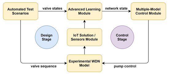
Figure 1.
Proposed solution pipeline.
The design stage is represented by the automated test scenarios for training the AI models on the experimental WDN, simulating consumer demand patterns and evaluating the network configuration from sensor data; the experimental results are in Section 4.3. The control stage is focused on the application of AI models in a multiple model control supervisor for regulating the pump based on the predicted state of the network and real-time sensor data; see the experimental results in Section 4.4.
The advanced learning module is based on machine learning and deep learning methods, described in Section 3.1 and Section 3.2. The multiple-model control module is based on the extension of the adaptive control strategy described in Section 3.4. The consideration of hydraulic modeling is presented in Section 3.3 and the evaluation methods include classification accuracy and control evaluation metrics in Section 3.5. The IoT Solution and the experimental WDN model are described in Section 4.1, and the automated test scenarios are defined in Section 4.3.
The main challenge in this design process is given by the different types of consumers and associated demand patterns during the day, accounting for a combination of operating conditions which can be translated into different control parameters for efficient pump operation.
Machine and deep learning models can both be used for classification problems such as detecting the network configuration in complex water distribution systems, as shown in the experimental results. There are multiple algorithms and mathematical models for the internal representation of data in the context of supervised learning and classification problems, such as decision trees and neural networks. To cover a broad range of different classification techniques, we chose as follows:
- For machine learning, we use a decision tree classification algorithm to have a baseline for the performance evaluation. Then, we use the random forest classification algorithm to see whether combining multiple classifiers using an ensemble method improves the accuracy of prediction.
- For deep learning, we use a multi-layer perceptron to have a baseline for the neural network models and see if it outperforms the classic machine learning algorithms. Then, we use a recurrent neural network (RNN) with multiple LSTM layers to determine whether a deep neural network architecture is a good fit for our problem and whether it outperforms both classic machine learning algorithms and the multi-layer perceptron.
For a given consumer node (or multiple consumers associated with a pumping station), it is important to evaluate the state of the network and the general operating conditions, to be able to predict the optimal control strategy with regard to the proposed control objectives (i.e., stability, transient response, overshoot, steady-state error).
The hydraulic model of laminar flow through pipes is considered for controller design and evaluation of results in terms of the equivalent process model. The consideration of the physical dimensions of the experimental model defines the context of the results and the applications in large scale WDNs.
The multiple model control is a subset of adaptive control, based on a supervisor for model/controller switching. Controller selection can be achieved using the model output error in classical solutions based on control theory, as well as machine and deep learning models in data science based solutions.
In the following subsections, we present the background for the algorithms and methods used in this paper for the experimental results.
3.1. Machine Learning Models
Machine learning is a subset of AI with a focus on learning from experimental data. There are multiple classes of algorithms for supervised (classification, regression) and unsupervised (clustering) learning problems, based on different mathematical models for data representation.
3.1.1. Decision Trees
A classification model can be build in the form of a decision structure using a decision tree classifier. The process of building such a tree includes the following steps: (i) break down each dataset into smaller subsets; (ii) associate each node to the attribute for which the best split is found; (iii) add a number of branches equal to the number of distinct values of that attribute for each node. When all the observations in a subset or a majority of them have the same class, then the node becomes a leaf labeled with the class name.
ID3 [48] is an algorithm that constructs a decision tree in a top-down manner by computing at each split the homogeneity of similar values using entropy. Given a set of classes , where , and a labeled dataset , where with each observation containing attributes , the entropy is with the probability of class in the dataset X. If attribute having r distinct values is considered for branching, it will partition X in r disjoint sets . The entropy of the split is given by with the proportion of elements in to the number of elements in the dataset X. Because the purity of the datasets is increasing, is bigger than . The difference between them is called the information gain . The maximum gain determines the best attribute for the split. C4.5 [49] is the improved version of ID3 that handles numeric continuous attributes and missing values, and performs post-pruning to deal with noisy data.
CART [50] (classification and regression tree) works on the same principles as C4.5 and ID3. The main difference is in the function used for calculating the homogeneity of a sample to compute the best attribute for the split. CART uses the Gini impurity: . The Gini impurity for a split is . In the case of CART, the split is done for the minimum Gini impurity.
Decision tree algorithms are greedy, meaning that they lead to a local optimum because attributes with many values lead to a higher gain.
3.1.2. Ensemble Methods
Ensemble methods combine multiple classifiers to obtain a better one. Combined classifiers are similar (use the same learning method) but the training datasets or the weights’ examples are different. Ensemble methods use Bagging (bootstrap aggregation) and boosting.
Bootstrap uses statistical methods (e.g., mean and standard deviation) for estimating a quantity from a data sample. Given a sample of n values we can compute its mean as . If n is small, then the sample mean has an error. The estimate of the mean can be improved by using bootstrap. Bootstrap will (i) create multiple random sub-samples of the initial sample with replacement, meaning the same value can be selected multiple times, (ii) calculate the mean for each sub-sample and (iii) calculate the average of all the sub-samples’ means and use it as the estimated mean for the initial sample.
Bootstrap aggregation (bagging) [51] is a machine learning ensemble algorithm designed to improve the stability and accuracy of machine learning that constructs a training set from the initial labeled data set by sampling with replacement. Bagging reduces the variance and helps to avoid overfitting. Bagging consists of: (i) starting with the original dataset, building n training datasets by sampling with replacement (bootstrap samples); (ii) for each training dataset, building a classifier using the same learning algorithm; (iii) the final classifier is obtained by combining the results of each classifier by voting for example.
The random forest classifier [52] is an ensemble classifier consisting of a set of decision trees. The final classifier outputs the modal value of the classes output by each tree. The random forest algorithm changes the selection of the split-point so that the learning algorithm, i.e., the decision tree classifier, is limited to a random sample of features with which to search. Thus, the algorithm constructs sub-trees that are less correlated.
3.2. Deep Learning Models
Deep learning is a subset of AI with a focus on learning from experience. Deep learning architectures stack together multiple layers of processing units to construct a supervised or unsupervised learning model. Depending on the number of states a processing unit incorporates, they vary from simple to complex.
3.2.1. Deep Feed Forward Network
The perceptron is one of the simplest processing units. It processes the input data X, encoded in a way that facilitates the computation, to predict an output y. For each features vector of dimension m, we can model a the predicted output of a perceptron as where is a weight vector; b represents the bias; and is the activation function, which takes the total input and produces an output for the unit given some threshold. The most popular activation functions are (i) the sigmoid , (ii) the hyperbolic tangent , (iii) the rectified linear unit (ReLU) and (iv) softmax with m the dimension of vector z. At each iteration, the loss or cross entropy function is used to adjust the weights when the real labels y are known, as shown in Equation (1).
A multi-layer perceptron neural network is an artificial neural network architecture that stack multiple layers of perceptrons. The basic architecture stacks three layers: (i) the input layer, (ii) the hidden layer and (iii) the output layer. All the nodes in one layer are fully connected to the neighboring layers using a certain weight , where i is the node and j is the layer. The multi-layer perceptron architecture is feed forward because the connections between the layers are directed from the input to the output. Each processing unit is a non-linear activation node. By adding multiple hidden layers, the architecture becomes a deep feed forward neural network architecture.
3.2.2. Long Short-Term Memory
Recurrent neural networks are artificial neural network architectures derived from deep feed forward neural network architectures and incorporating an internal state known as memory to process sequences of inputs. Among the most used cells for constructing such a network are the recurrent unit (RU) [53], the long short term-memory (LSTM) [54] and gated recurrent units (GRU) [55].
The LSTM uses two state components for learning the current input vector: (i) a short-term memory component represented by hidden state and (ii) the long-term memory component represented by internal cell state. The cell also incorporates a gating mechanism with three gates: (i) input gate (), (ii) forget gate () and (iii) output gate (). Equation (2) presents the state updates of the LSTM unit, where:
- is the input features vector of dimension m;
- is the hidden state vector as well as the unit’s output vector of dimension n, where the initial value is ;
- is the input activation vector;
- is the cell state vector, with the initial value ;
- are the weight matrices corresponding to the current input of the input gate, output gate, forget gate and the cell state;
- are the weight matrices corresponding to the hidden output of the previous state for the current input of the input gate, output gate, forget gate and the cell state;
- are the bias vectors corresponding to the current input of the input gate, output gate, forget gate and the cell state;
- is the sigmoid activation function;
- is the hyperbolic tangent activation function;
- ⊙ is the element wise product; i.e., Hadamard Product.
3.3. Modeling of Laminar Flow in Pipes
Laminar flow is often encountered in WDNs and consists of a regular flow pattern that is also easier to model than turbulent flow. The equations and methods presented can be found in the literature in the context of hydraulic modeling and control systems for industrial applications, as defined in [56,57].
Considering the following notations, the dynamic models of laminar flow through pipes are classified by the physical characteristics into: laminar flow through short pipes (where ) and laminar flow through long pipes (where ), where:
- L is the length of the pipe;
- D is the diameter of the pipe;
- is the fluid density;
- S is the pipe section.
The following notations are used to describe the equations for laminar flow:
- F is the flow through the pipe;
- is the reduction in pressure along the pipe;
- is the flow coefficient;
- is the flow velocity;
- is the fluid mass;
- is the fluid volume in static conditions.
3.3.1. Laminar Flow in Short Pipes
The hydraulic resistance of a short pipe is defined as .
The equations in static and dynamic equilibrium describe the process of laminar flow through a pipe segment:
The deviation from the static model can be written as follows:
Then, the equation for dynamic equilibrium is updated:
After replacing from the static model, the quadratic term is reduced and the equation becomes:
The input and output variables of the dynamic model are normalized based on the static conditions:
The dynamic model equation in differential form is then written as follows:
We apply the Laplace transform to obtain the transfer function of the process model:
where:
- is the process gain;
- is the time constant of the process.
3.3.2. Laminar Flow in Long Pipes
The hydraulic resistance of a long pipe is in this case mostly determined by the pipe length and defined as where k is the coefficient of friction.
The equations in static and dynamic equilibrium describe the process of laminar flow through a long pipe:
The deviation from the static model and reduction of the quadratic term is similar to laminar flow through short pipes and the equation for dynamic equilibrium is updated:
The dynamic input output model in differential form is then written as follows:
We apply the Laplace transform to obtain the transfer function of the process model:
where:
- is the process gain;
- is the time constant of the process.
3.3.3. Consideration of Process Model
The process model is defined in the context of the experimental model as a combined model of laminar flow through multiple pipes. As the consideration is for a laminar flow through short pipes, the process time constant for laminar flow is small when compared to that of the actuator elements (pump, valves). It is also considered as a simplified model with reduced nonlinearities (e.g., quadratic term) in the process model, which is commonly used for traditional controller design.
For the control model design, the transfer function of the fixed part is defined by the laminar flow model (, first order), actuator element (, first order) and sensor model (, constant).
In the context of large scale WDNs, the design process is similar from the perspective of control systems, in the sense that the time constant is adjusted according to the laminar flow model in long pipes.
3.4. Multiple Model Control
In multiple model control strategies, the supervisor (switching block) has to ensure fast and accurate switching of the control algorithm according to the current state and operating regime of the process [58]. There are some additional requirements for smooth operation and scalability of such architectures. A bump-less transition and an efficient strategy for activating the controllers is often required for control applications.
The architectures for multiple model control can be classified as the traditional structure, based on modeling and simulation and the proposed AI-based solution for implementing the supervisor, as presented in Figure 10. In the traditional multiple model control structure, the first step is to evaluate the static input–output characteristic of the process. The problem of nonlinearities and discontinuities, given by, e.g., the different operating regimes is solved by constructing multiple models, each with a different transfer function given the piecewise linear approximation of the dynamic input–output characteristic of the process , where [59]. The model output error is defined relative to the process output at sample k as in Equation (17). For each model, there is an ideal controller that satisfies the control objectives while only some of the outputs are actually applied on the real process according to the switching block. The objective function in Equation (18) defines the ideal criterion for model selection in discrete time. In operating conditions, the selection is based on the model output error, by comparing model outputs to the process output. The multiple model controller output is based on the evaluated outputs and weights for each associated controller, as shown in Equation (19), where:
- is the process output at sample k;
- is the output of model i at sample k;
- is the output error of model i at sample k;
- is the controller output for model i at sample k;
- is the controller weight for model i at sample k;
- is the weighting factor;
- is the long term accuracy for instantaneous measurements;
- is the forgetting factor for active window limitation over the model error .
In the most simple form, a single controller is selected at any given time based on the output error of the associated model. This method requires additional processing for the transition between selected models to ensure robust operation and reduced discontinuities in the controller output [60].
With the AI-based supervisor, using the classification methods described in Section 3.1 and Section 3.2, the probability vector can be used directly to apply the model weights for mixing controller outputs, i.e., , or adapted for switching strategies with a single active controller by selecting the model having the highest probability .
3.5. Evaluation Methods
The following methods are used to evaluate the classification algorithms and the application of AI methods in a multiple model control strategy for pumping stations.
3.5.1. Classification Evaluation Metrics
The network configuration is defined as a combination of valve states according to the consumer demand patterns, and is translated into a multi-class classification problem in the context of model selection for multiple model control.
In the context of machine learning, evaluation methods must be defined based on the type of model employed by the machine learning task; i.e., classification, regression or clustering. To properly evaluate a classification task, the type of classification must be identified using one of following four categories [61]: (i) binary, (ii) multi-class, (iii) multi-labeled and (iv) hierarchical.
For binary classification, an observation is assigned to one of two classes: or . The evaluation is performed using the confusion matrix containing the following information: (i) (true positive) and (true negative) are the observations labeled with and , correctly classified; (ii) (false negative) is the number of observations labeled as classified as ; and (iii) (false positive) is the number of observations labeled as classified as . Using the confusion matrix, the accuracy is defined as .
For multi-class classification, a data point is assigned to one of multiple classes , with and as the number of classes. A confusion matrix is built containing the values , , and belonging to each class . In the case of multi-class classification, the accuracy is defined as .
The evaluation of multiple methods for detecting the network configuration is based on the accuracy for each dataset and a cross-validation on the other datasets, as described in the results section. The best model in terms of overall accuracy is evaluated on a random dataset with consideration of real operating conditions in a WDN.
3.5.2. Control Evaluation Metrics
The classification model is used for controller selection in the proposed AI multiple model controller for pumping stations. The evaluation metrics for the closed loop response are defined as the steady state error ( in Equation (20)), overshoot ( in Equation (21)) and standard deviation ( in Equation (22)) used for the evaluation of closed loop performance [62,63].
where:
- is the overshoot;
- is the steady state error;
- is the (steady state) controller setpoint;
- is the steady state closed loop response;
- is the maximum closed loop response with regard to the steady state;
- is the standard deviation of the controller output in discrete time;
- is the discrete controller output at sample k;
- is the mean controller output.
4. Results
The results are based on the experimental water network model described in Section 4.1 with applications including the evaluation of control algorithms for pumping stations, leak detection and network configuration. We describe the multi-domain approach that combines IoT integration, automated test scenarios for evaluation of advanced learning methods and the extension of multiple model control for pumping stations as described in [47]. The scenarios cover the entire range of consumer demand patterns that can be achieved by opening and closing the valves with binary (gray code) sequence. However, there are other possible sequences, emphasized by the random experiment in Figure 9, which can be defined upon initial evaluation of consumer demands in a real WDN.
4.1. Experimental Model
The water network construction is based on detachable elements: PVC (polyvinyl chloride) pipes, couplings, valves and water flow sensors that can simulate consumer demands and leaks, as shown in Figure 2. The experimental WDN schematic in Figure 3 is designed for the evaluation of multiple consumer demands with nodes, pipes and valves in a complex layout with several loops (e.g., J1-J6-J11-J12), limited in scale by the dimensions of the board. A DC electrical pump (P0) is used to provide the water supply for the entire network and a supply tank (T0) is used for closed loop operation. Valves (V1-V6) can be used to simulate both consumers and leaks, depending on the evaluation scenario and the scope of the experiments. Sensors are mounted along the pipes (S0-S9) to measure the flow for both junctions (J0–J18) and consumer nodes (C1–C6). The configuration allows for the evaluation of leak detection capabilities (e.g., leak sensitivity analysis), consumer demand estimation (e.g., cluster analysis) and control algorithms (e.g., multiple model control), in the context of water booster pumping stations for handling peak flows in residential areas.
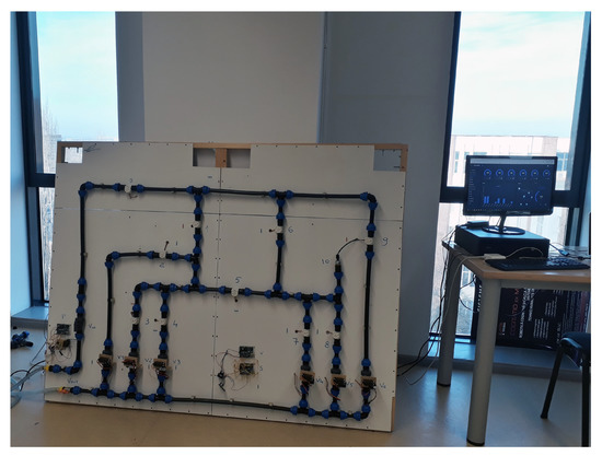
Figure 2.
Experimental model.
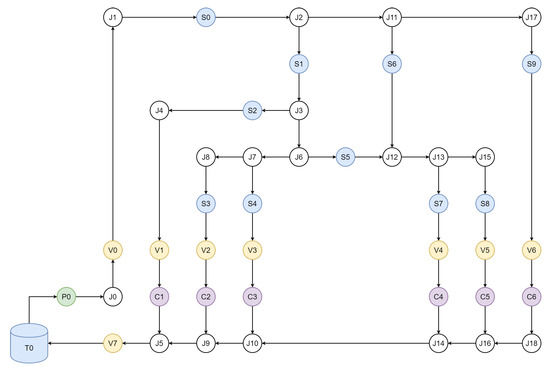
Figure 3.
Experimental model schematic.
The sensors, pump controller and servo-valves are connected to the IoT network using Arduino boards and ESP8266 Wi-Fi modules. With large scale WDNs that are geographically distributed and placed underground, measurement nodes can be designed with GPS, local storage and long distance network transceivers (e.g., LoRa, 5G); data aggregator nodes are often required for interfacing with cloud platforms. Transmission errors, power outages and network availability have to be considered for large scale deployments and continuous operation, while ensuring data retention and synchronization [64].
For the experimental model, measurement nodes consist of YF-S201 flow sensors with a range of 1 L/min to 30 L/min, connected to an Arduino board. The flow sensors contain a rotor and a hall sensor which converts the water flow into electrical pulses. The sensor signal is then read by the microcontroller using pin change interruptions and hardware timers for measuring the time between consecutive pulses, as shown in Equation (23), for Timer1 of the Atmega328p, configured in CTC mode with top at OCR1A. The timer units are converted to using the linear approximation of the static input–output characteristic of the sensor, i.e., , as shown in Equation (24). As the timer counter is reset every 10 ms, upon each interruption a software counter is incremented to count larger periods of time for each connected sensor.
where:
- is the flow in at sample k;
- is the counter value at sample k;
- is the timer interrupt frequency—i.e., 100 Hz;
- is the clock frequency—i.e., 16 MHz;
- is the clock prescaler—i.e., 64;
- is the counter limit—i.e., .
The choice of flow sensors is based on the higher accuracy when compared to pressure sensors at this scale. The ESP8266 Wi-Fi adapters are connected to the Arduino boards and provide MQTT connectivity for remote control and monitoring.
For the automated test scenarios required for the evaluation of advanced learning methods in Section 4.3 and multiple model controller design in Section 4.4, the manual valves were converted to servo-valves using Turnigy TGY-AN13 DC servos directly attached on top, which required adjustment to the electrical wiring and using a dual supply for powering the sensors and control boards. The mechanical design is reliable and provides good precision for automated testing involving on/off operation of valves and incremental positioning, making the solution a good alternative to solenoid valves. As there is inherently a moderate level of mechanical hysteresis, dynamic compensation was added in software. An additional valve was added on the return path for increased control on the water pressure across the entire network.
4.2. Reactive IoT Platform
For monitoring the parameters in the water network, and a real-time framework for control applications, the IoT platform was designed with reactive components and publish–subscribe data exchange models. The platform provides interaction with the physical components (pump, sensors, valves), real-time control and monitoring, automated testing and data storage capabilities.
The IoT nodes are connected using a Wi-Fi access point and the MQTT broker installed on a Raspberry Pi board. The data exchange is facilitated by the MQTT broker, using a publish–subscribe model, allowing for a standard interface and interoperability with other services.
The application server is written in Python and handles the interaction with the IoT devices through MQTT, providing data storage and automated testing capabilities as well as the integration of high-level data processing frameworks such as TensorFlow, Keras and scikit-learn [65]. There is, however, an inherent limitation for handling high throughput input/output operations; e.g., updating the database and running control loops on separate threads, given by the single-thread global interpreter lock (GIL) in Python. With some adjustments and reactive programming patterns, the sampling time of 100 ms was ensured during the experiments.
The UI is implemented using Angular, providing an asynchronous framework based on TypeScript that is more extensible and structured than other JavaScript-based frameworks. It is based on the admin dashboard template ngx-admin that uses the Nebular UI components, handling most visual elements and themes on top of the Angular framework [66]. The main features include MQTT connectivity; graphical widgets for interacting with sensors, valves and pumps; and the control panel for experimental setup.
The real-time data exchange is implemented using WebSockets and reactive extensions. The UI and server are designed to support integrated push-based events, such as showing experimental progress in real-time.
4.3. Evaluation of Advanced Learning Methods
The primary objective of this stage is to evaluate the performance of advanced learning methods for detecting the network configuration in real-time from smart meter measurements in terms of the prediction accuracy, storage and processing requirements for real-time operation. The evaluation is based on automated test scenarios for the water network model and provides initial results for replacing the traditional multiple model control supervisor.
During the automated experiments, the data from measurement nodes and the state of the actuators was collected in the database with the associated timestamps. The experimental data generated in the first scenario (1-N) are shown in Figure 4. The sampling is time-based, capturing the transient response and the steady state measurements.
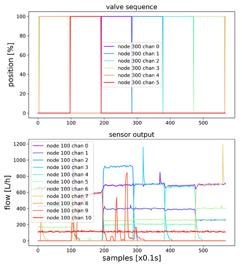
Figure 4.
Experimental data.
The scenarios involve programmed valve opening patterns to simulate changing network configuration in terms of variable consumer demands. There are several patterns that are used for extensive evaluation of learning capabilities in a complex network, from simulating single consumer scenarios with only one active consumer, towards a full range of binary combinations involving the six servo-valves that are installed on the experimental model. As the binary operation already provides a wide range of combinations (), the AI models are designed to predict the combination of the on/off states of the valves for this scope.
Each scenario is run multiple times on the experimental model to achieve better results in terms of overfitting, and between each step there is a constant delay of 10 seconds, which allows the entire network to reach steady state in terms of water flow. However, there is no preprocessing involved, as each sample is used to train the models, including the transient states obtained when switching valves.
The proposed scenarios for simulating consumer demand patterns are designed starting from the most simple pattern represented by a single consumer node that is active at any given time, and extended to include the entire range of binary combinations, with variable pump output to provide better cross-validation and evaluation for real operating conditions:
- 1-N (one way single valve sequence). The valves are opened and closed in sequence, starting from the first valve up to the last valve. The next valve is opened and the current valve is closed, with no delay in between, accounting for the transient state in network reconfiguration. The pump is set to 80% for the duration of the experiment.
- 1-N-1 (single valve return sequence). The valves are opened and closed in sequence, starting from the first valve up to the last valve, and then going back to the first valve. This case is evaluated for 80% and 50% pump outputs.
- GRAY (gray code valve sequence). The valves are opened and closed according to the 6-bit gray code, so that consecutive combinations differ by a single valve and the entire range of combinations is achieved. The pump is set to 80% for the duration of the experiment.
The next step involves evaluating advanced learning models using the experimental data to predict the network configuration in real-time. The accuracy and processing requirements are evaluated and the models are compared to provide insights about the performance that can be achieved in the context of a complex network model. Flow measurements are input variables; valve states are used as target variables for the models; and the dataset is divided into training, validation and test samples. For each scenario, multiple models are trained, and the best model is presented, along with the average model, in terms of prediction accuracy.
The classification problem implies that there are multiple classes and each input can belong to exactly one class (multi-class classification). Therefore, the target datum is encoded, using integer encoding and one-hot encoding of the binary combination of valves to represent each network configuration. The models are representative of the major approaches to supervised learning which we refer to as machine learning methods and deep learning methods.
In this multi-class classification problem with more than two exclusive, one-hot encoded classes, the categorical cross-entropy loss function is used for training deep learning models. According to [67], the number of hidden layers can be selected to “represent an arbitrary decision boundary to arbitrary accuracy with rational activation functions.” A number of three hidden layers was found to provide better results for cross-validation, when compared to a configuration with two hidden layers. The Keras library was used with Python to train and evaluate deep neural network models:
- Dense. For the deep feed forward network, i.e., a dense model, a multi-layer perceptron (MLP) is used for multi-class softmax classification. Three hidden layers are used with a dropout rate of and 32 units. The hidden layers use a ReLu activation function, while softmax is used for the output layer, which gives the outputs as probabilities. The model is implemented in Keras as a Sequential model using dense layers. The model is trained in a maximum of 500 epochs with a stop criterion implemented as EarlyStopping monitor based on the loss function (categorical_crossentropy for multi-class classification).
- RNN. A recurrent neural network (RNN) is implemented as a sequential model with three LSTM hidden layers, while the output layer is a dense layer with a softmax activation function. The two dimensional input data (samples, sensor nodes) are reshaped into a 3D representation that is required for training the model. While the LSTM model has a higher learning rate when compared to the dense model, it is more intensive in terms of computation, and therefore it is trained using a fixed number of five epochs using the categorical_crossentropy loss function.
The multi-class classification problem is directly solved by using machine learning classifiers with the integer encoding of network configurations; i.e., . The multiple target variables in the case of one-hot encoding are translated into a single target classification problem with integer encoding. The scikit-learn library is used with Python to train and evaluate supervised and unsupervised learning models:
- DT. A decision tree classifier is implemented using the DecisionTreeClassifier in scikit-learn, with a default splitting criterion based on the Gini Index. The accuracy is evaluated in terms of the predicted classes for the integer encoded test dataset.
- RF. A random forest classifier is implemented using the RandomForestClassifier in scikit-learn, with a default splitting criterion based on the Gini Index and 100 estimators. The accuracy is evaluated in terms of the predicted classes for the integer encoded test dataset, while the model aims for improved accuracy and reduced overfitting when compared to a single decision tree.
The comparison between the proposed learning methods on the matching dataset (the same scenario is used for training and validation) is shown in Figure 5a for average model evaluation and Figure 5b for best model evaluation.
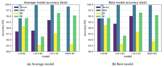
Figure 5.
Accuracy evaluation.
The RNN model (blue) is superior to the dense model (purple), and the RF model (green) shows higher accuracy than the DT model (yellow), as shown in Figure 5a. The dense model shows unexpected results for the GRAY test scenario, showing considerably lower accuracy than the other models for the classification problem. In the best model chart in Figure 5b, the results are similar. The RNN model is more consistent and outperforms the other models in every scenario, for both average and best model evaluations, while the RF model shows surprisingly good results in this evaluation.
An interesting result was observed for each model with the 1-N-1 test scenario where the accuracy is better for the dataset obtained with 50% pump output, which can be explained by the reduced pressure and therefore less disturbance during transient state of valve switching.
An overview of the model evaluation is presented in Figure 6, with Figure 6a showing a combined accuracy for each model resulting from the average of each matching dataset, with a side-by-side comparison between the best (blue) and the average (purple) models. The average results for each method are as follows: dense (average 68.76%, best 72.89%), RNN (average 99.61%, best 99.79%), DT (average 86.11%, best 86.83%), RF (average 93.13%, best 93.35%). In Figure 6b, the combined accuracy (circle size), training time (y axis, linear scale) and storage requirements (x axis, logarithmic scale) are shown for each model as a 2D XY plot. The RNN model (blue) is the most expensive in terms of computation (training time: 112 s) and the RF model (green) requires the most storage space (28.3 MB). Machine learning models are generally less expensive in terms of computation time when compared to deep learning models in this evaluation.
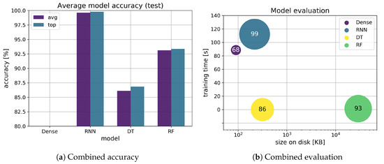
Figure 6.
Evaluation overview.
For an extensive evaluation and cross-validation, each model trained on a matching dataset was tested on the other test scenarios as well. The results are presented in Figure 7 (the deep learning models), and Figure 8, in which the machine learning models, in a colormap representation (YlGnBu color scheme), show the model on the y axis and the dataset that is used for evaluation on the x axis. Each model and dataset is labeled according to the coresponding test case. A higher accuracy of a given combination of model and dataset is shown in blue and a lower accuracy is shown in yellow, relative to the associated scale.
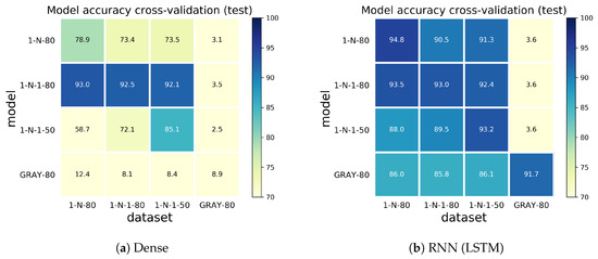
Figure 7.
Cross-validation (deep learning).
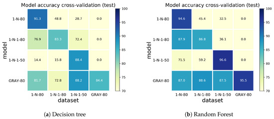
Figure 8.
Cross-validation (machine learning).
The dense model shows similar performance, with considerably lower accuracy, to the RNN model for the classification problem. The results show higher overfitting for machine learning models and comparable lower accuracy while the deep learning models are able to predict other datasets with good accuracy. The RF classifier, however, shows good accuracy and less overfitting than the DT classifier. In fact, the average accuracy for cross-validation test is as follows: dense with 47.87%, RNN with 74.16%, DT with 65.15% and RF with 74.54%.
A general trend was observed: that a higher coverage of possible consumer demands is required for predicting unknown test scenarios. The models that are trained on the single valve sequence (1-N, 1-N-1) are not able to predict combinations of valves when compared to models that are trained on the entire range of valve combinations (GRAY). However, with the RNN model, both the single valve class of models and the GRAY model yield similar results on the 1-N and 1-N-1 datasets, showing good adaptability to different scenarios having similar configurations. The RF classifier achieves good accuracy for the GRAY model across the experimental dataset, showing less overfitting than the DT/GRAY model and comparable results to the RNN/GRAY model in this case.
The next step was to evaluate the model in a random test sequence in terms of accuracy in real operating conditions. Unlike the automated test scenarios that were used to train the model, this is a manual test that covers some additional characteristics, such as variable timing and random changes between combinations of on/off valves, as shown in Figure 9.
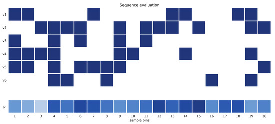
Figure 9.
Random test sequence evaluation.
The colormap representation of valve states and prediction accuracy is shown for a subset of samples equally distributed across the dataset. The prediction accuracy is represented using different shades of blue for each column as the average prediction accuracy for the associated samples (Blues color scheme). The RNN model was considered for this evaluation—it was the most accurate to this point—and the results show an average prediction accuracy of 70%. This leads to the conclusion that the proposed test scenarios do not cover all possible situations that may be found in real operating conditions; therefore, the model’s performance is limited by the dataset that is used for training. Considering that the training datasets have a moderate amount of 10,000–20,000 samples, the model performance shows promising results. A higher number of samples can be achieved by a random test scenario with variable timings and combinations of valves.
The main scope of using machine learning and deep learning models in this article entailed providing the current state of the network, described by the combination of valves, for multiple model controller switching, as presented next in Section 4.4.
4.4. Extension of the Multiple Model Control Structure
In the proposed scenario, with consideration of the process models and control systems, as described in Section 3.3 and Section 3.4, a multiple model control structure is used to control the pump, regulating the pressure for a consumer node, providing increased adaptability to the network configuration. As the configuration of the network is based on the complex structure and actual demands during the day, there can be multiple models that characterize each operating condition, with a supervisor that handles the selection of the most suitable controller.
The extension of the multiple model control supervisor is based on the learning models evaluated in Section 4.3. The decision support provided by learning methods can be used to either enhance or replace the more traditional supervisor based on the output errors of simulated models. The supervisor, in this case, is represented by the learning model and an adaptation module. The inputs to the supervisor are provided as real-time measurements from sensor nodes, and the outputs represent the predicted network configuration in the form of one-hot encoded probability vectors, which are then used to activate the controllers. In this case, the AI model replaces the real-time process model evaluation, as shown in Figure 10. This method provides a decoupled architecture for the multiple model control strategy as follows:
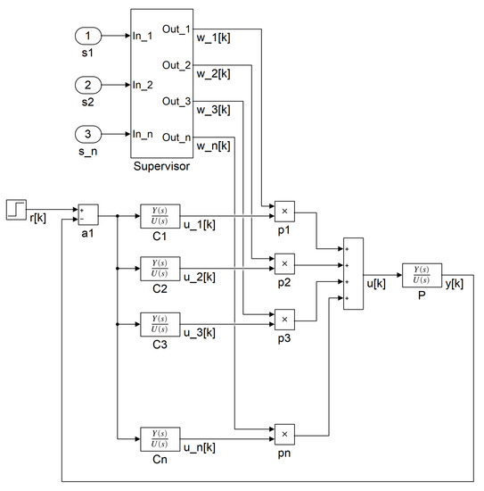
Figure 10.
Multiple model controller schematic.
- Controller design is based on experimental identification or closed-loop PID tuning strategies for first and second order models. For first order models having the transfer function of , the methods include evaluation of step response for calculating the amplification factor K and time constant T and using pseudorandom binary sequence (PRBS) applied to the process for more advanced and automated identification. For PID tuning, the closed loop response is evaluated, and the coefficients , and are adjusted to match the performance criteria (asymptotic error , settling time and overshoot).
- Controller selection is based on learning from simulated scenarios, aiming at improved adaptability and replacing or complementing the more traditional switching algorithm based on model outputs. In this case, the RNN model returns the probabilities for each class at each sample k, which are then used for switching (on/off, weighted output) the associated controllers. Classes () define network configurations, represented as one-hot encoded binary combinations of valves; i.e., .
The experimental setup consists of a target consumer node for which a reference flow has to be maintained during changing operating conditions given by the network configuration. The other valves, i.e., consumer nodes, are opened in sequence to simulate individual consumers that are active at the same time.
The results with RNN model supervisor and multiple PID controllers are shown in Figure 11. The control data (measured flow and pump output) are represented on the plot with state transitions shown by the vertical lines, while the predictions (predicted models and accuracy) are represented on the colormap chart.
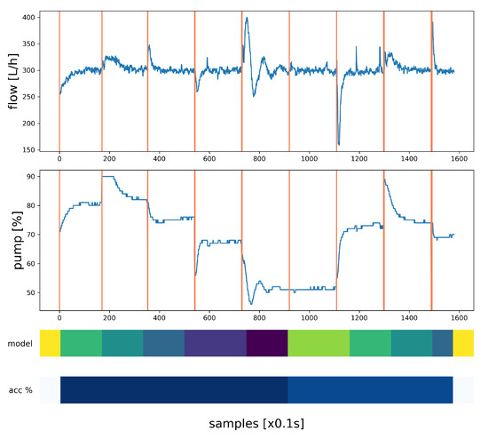
Figure 11.
Control integration experiment.
In this evaluation, the switching is based on the best controller selection obtained using the highest probability index, and the RNN is trained on the control scenario to obtain the required accuracy. Using the previous models resulted in less accurate predictions, which can be explained by the different operating conditions that were not captured in the automated test scenarios.
The controller shows improved transient response and adaptability to changing network configuration when compared to a simple PID (proportional-integral-derivative) structure. The control objective defined for disturbance rejection when switching valves, is satisfied with the multiple model controller with a combined (calculated from each actual network configuration) zero steady state error; an average overshoot within 5% of the target output—i.e., measured flow within the consumer node; and an average standard deviation of 11.2% for the command—i.e., pump output [%].
5. Discussion
The results are promising for the adaptability of machine and deep learning models to the complex problem of predicting the network configuration in complex WDNs. While the simulated scenarios cover the possible configurations of the experimental model, there are many more variables in the context of real operating conditions, as emphasized by the random test scenario. Training the models often requires large amounts of data for achieving a good accuracy in practical applications, which is important to consider in production environments.
While neural networks are able to represent complex models given large amounts of data for training, the network architectures, activation functions, optimization algorithms, number of nodes and hidden layers play important roles in achieving good accuracy and having adaptability to changing operating conditions. Machine learning classifiers often require less tuning and computational effort, and represent an alternative to more complex deep learning models that often require large training sets to be effective.
With the experimental model, the conditions can be achieved for generating a large dataset with variable configurations and timings, to allow for obtaining excellent prediction accuracy, while in large scale WDNs there can be additional challenges and restrictions.
In the context of multiple model control for pumping stations, using machine and deep learning models represents a shift from the traditional model identification and evaluation based on short-term experimental data, to a more data-oriented solution for designing the supervisor, while covering a broad range of operating conditions. Provided that the models are trained on a large enough dataset, this method is superior from the perspective that it provides improved decision support for the controller switching strategy. However, in large scale WDNs, this can require lots of experimental data for training accurate models, including variable timings, operating conditions (e.g., pump output) and valve sequences.
The controller selection is defined as a multi-class classification problem adapted for neural networks using one-hot encoding and the predictions are used to activate the controllers according to the probability vector. As each correct prediction assumes that a combination of valves is matched, the categorical cross-entropy loss function leads to an accurate evaluation of accuracy in real operating conditions, as demonstrated in the experimental results.
The process models obtained for different network configurations in the experimental WDN are similar with regard to the transient response, and the controllers are simple to design, while this may not be the case in large scale WDNs. This aspect is revealed by the physical characteristics with laminar flow in short pipes, as presented in Section 3.3, while the same approach can be used for more complex configurations as well. While a traditional approach based on experimental methods for system identification in the case of controller design can prove to be a tedious task for complex systems, there are some promising results from the domain of reinforcement learning that can provide highly adaptable control structures [68].
6. Materials and Methods
The hardware and mechanical design of the experimental model is presented in Section 4.1, and the software components for real-time control and monitoring are based on the latest technologies in web development, described in Section 4.2. The experimental data are collected into a MySQL database and then extracted as CSV files for training the machine and deep learning models and evaluating the prediction accuracy and control performance of the multiple model control supervisor.
The source code, experimental data and results obtained during the experimental evaluation are available on GitHub (WDN Model Experiments: https://github.com/alexp25/wdn-model-experiments). The code is compatible with Python 3.6 and is organized into multiple independent scripts, modules and configuration files for evaluating the experimental data from CSV files. The deep learning models are trained using Keras and TensorFlow, while scikit-learn is used for training the machine learning models. The Matplotlib library is used for visual representation of the results as plots, bar charts and heatmaps, according to the evaluation type (raw data, comparison, cross-validation and prediction).
7. Conclusions
Smart water networks represent the next step in the development of essential infrastructure in the context of smart cities, requiring modern solutions and the convergence of multiple domains of research for efficient management and operation. A literature review reveals some key aspects that are subjects of ongoing research in the domains of IoT solutions, smart meters, advanced learning methods and control systems.
Starting with the IoT infrastructure, the development of modern, streamlined platforms is based on publish–subscribe and push-based architectures across the entire IoT stack, and reactive programming patterns for real-time applications. Smart meters and actuators are presented in the context of an experimental WDN. An alternative to the solenoid valves was developed by converting a manual valve into a servo-valve with incremental positioning.
The proposed experimental WDN model also provides an excellent test bench for the evaluation of control and prediction algorithms that exist in the literature. Automated testing is an important component for the industry and the evaluation of the experimental WDN. The proposed test scenarios were used to evaluate machine and deep learning models for predicting the network configuration in the context of a multiple model control supervisor for pumping stations. A good accuracy was obtained using the raw experimental data, and the models were compared in terms of the overall accuracy, the cross-validation test and the processing and storage requirements, showing promising results in terms of the adaptability of such models in complex WDNs.
The multiple model control strategy allows for a decoupled architecture with improved adaptability for complex WDNs of various configurations. Models and controllers were designed for different operating conditions, and the closed-loop controller selection is handled by the proposed supervisor using advanced learning methods.
Additional perspectives on the proposed experimental model include incremental positioning of the valves, network reconfiguration, demand estimation and leak detection using advanced learning algorithms.
Author Contributions
Conceptualization, A.P., C.L., C.-O.T. and E.-S.A.; methodology, A.P., C.-O.T. and E.-S.A.; software, A.P.; validation, A.P.; formal analysis, A.P., C.-O.T. and E.-S.A.; investigation, A.P.; resources, A.P., M.M. and C.L.; data curation, A.P.; writing–original draft preparation, A.P., C.-O.T. and E.-S.A.; writing–review and editing, A.P., C.-O.T., E.-S.A., M.M. and C.L.; visualization, A.P.; supervision, M.M. and C.L.; project administration, M.M. and C.L.; funding acquisition, M.M. All authors have read and agreed to the published version of the manuscript.
Funding
This research received no external funding.
Acknowledgments
The publication of this paper is supported by the University Politehnica of Bucharest through the PubArt program.
Conflicts of Interest
The authors declare no conflict of interest.
References
- Rode, S. Sustainable drinking water supply in Pune metropolitan region: Alternative policies. Theor. Empir. Res. Urban Manag. 2009, 4, 48–59. [Google Scholar]
- KALLIS, G.; COCCOSSIS, H. Water for the City: Lessons from Tendencies and Critical Issues in Five Advanced Metropolitan Areas. Built Environ. 2002, 28, 96–110. [Google Scholar]
- Kelman, J. Water Supply to the Two Largest Brazilian Metropolitan Regions; At the Confluence Selection from the 2014 World Water Week in Stockholm. Aquat. Proc. 2015, 5, 13–21. [Google Scholar] [CrossRef]
- Sun, G.; Mcnulty, S.; Myers, J.; Cohen, E. Impacts of Multiple Stresses on Water Demand and Supply Across the Southeastern United States1. JAWRA J. Am. Water Res. Assoc. 2008, 44, 1441–1457. [Google Scholar] [CrossRef]
- Awe, M.; Okolie, S.; Fayomi, O.S.I. Review of Water Distribution Systems Modelling and Performance Analysis Softwares. J. Phys. Conf. Ser. 2019, 1378, 022067. [Google Scholar] [CrossRef]
- Arsene, C.; Al-Dabass, D.; Hartley, J. A Study on Modeling and Simulation of Water Distribution Systems Based on Loop Corrective Flows and Containing Controlling Hydraulics Elements. In Proceedings of the 3rd International Conference on Intelligent Systems Modelling and Simulation, ISMS 2012, Kota Kinabalu, Malaysia, 8–10 February 2012. [Google Scholar] [CrossRef]
- Dobriceanu, M.; Bitoleanu, A.; Popescu, M.; Enache, S.; Subtirelu, E. SCADA system for monitoring water supply networks. WSEAS Trans. Syst. 2008, 7, 1070–1079. [Google Scholar]
- Martinovska Bande, C.; Bande, G. SCADA System for Monitoring Water Supply Network: A Case Study. Int. J. Softw. Hardw. Res. Eng. 2016, 4, 1–7. [Google Scholar]
- Camarinha-Matos, L.M.; Martinelli, F.J. Application of Machine Learning in Water Distribution Networks Assisted by Domain Experts. J. Intell. Rob. Syst. 1999, 26, 325–352. [Google Scholar] [CrossRef]
- Koo, D.; Piratla, K.; Matthews, C.J. Towards sustainable water supply: Schematic development of big data collection using internet of things (IoT). Proc. Eng. 2015, 118, 489–497. [Google Scholar] [CrossRef]
- Siddique, N.; Adeli, H. Introduction to Computational Intelligence. In Computational Intelligence; John Wiley & Sons, Ltd.: Hoboken, NJ, USA, 2013; Chapter 1; pp. 1–17. [Google Scholar] [CrossRef]
- Bunn, S.M.; Reynolds, L. The energy-efficiency benefits of pump-scheduling optimization for potable water supplies. IBM J. Res. Dev. 2009, 53, 5:1–5:13. [Google Scholar] [CrossRef]
- Ormsbee, L.; Lansey, K. Optimal control of water supply pumping systems. J. Water Res. Plann. Manag. 1994, 120, 237–252. [Google Scholar] [CrossRef]
- Walker, D.; Creaco, E.; Vamvakeridou-Lyroudia, L.; Farmani, R.; Kapelan, Z.; Savic, D. Forecasting Domestic Water Consumption from Smart Meter Readings Using Statistical Methods and Artificial Neural Networks. Proc. Eng. 2015, 119, 1419–1428. [Google Scholar] [CrossRef]
- Rahim, M.S.; Nguyen, K.A.; Stewart, R.A.; Giurco, D.; Blumenstein, M. Machine Learning and Data Analytic Techniques in Digital Water Metering: A Review. Water 2020, 12, 294. [Google Scholar] [CrossRef]
- Wu, Z.; El-Maghraby, M.; Pathak, S. Applications of Deep Learning for Smart Water Networks. Proc. Eng. 2015, 119, 479–485. [Google Scholar] [CrossRef]
- Avni, N.; Fishbain, B.; Shamir, U. Water consumption patterns as a basis for water demand modeling. Water Resour. Res. 2015, 51, 8165–8181. [Google Scholar] [CrossRef]
- Merit Solutions, Why a Holistic Approach is the Best Way to Achieve Manufacturing Transformation. Available online: https://meritsolutions.com/holistic-approach-manufacturing-transofrmation-blog/ (accessed on 24 January 2020).
- Loring, M.; Marron, M.; Leijen, D. Semantics of Asynchronous JavaScript. In Proceedings of the 2017 Symposium on Dynamic Languages, Vancouver, BC, Canada, 24 October 2017; pp. 51–62. [Google Scholar]
- Yu, L.; Qiu, H.; Li, J.H.; Chang, Y. Design of Asynchronous Non-block Server for Agricultural IOT. In Proceedings of the 2019 4th International Conference on Big Data and Computing, Guangzhou, China, 10–12 May 2019; pp. 322–327. [Google Scholar]
- Smith, J. Machine Learning Systems: Designs that Scale; Learning reactive machine learning; Manning Publications: Shelter Island, NY, USA, 2018; Chapter 1. [Google Scholar]
- Wu, Z.; Rahman, A. Optimized Deep Learning Framework for Water Distribution Data-Driven Modeling. Proc. Eng. 2017, 186, 261–268. [Google Scholar] [CrossRef]
- MIT Technology Review, Ten Breakthrough Technologies 2013. Available online: http://www.technologyreview.com/lists/breakthrough-technologies/2013/ (accessed on 24 January 2020).
- Predescu, A.; Negru, C.; Mocanu, M.; Lupu, C.; Candelieri, A. A Multiple-Layer Clustering Method for Real-Time Decision Support in a Water Distribution System. In Business Information Systems Workshops; Abramowicz, W., Paschke, A., Eds.; Springer International Publishing: Cham, Switzerland, 2019; pp. 485–497. [Google Scholar] [CrossRef]
- Seyoum, A.; Tanyimboh, T. Integration of Hydraulic and Water Quality Modelling in Distribution Networks: EPANET-PMX. Water Resour. Manag. 2017, 31, 4485–4503. [Google Scholar] [CrossRef]
- Giudicianni, C.; Di Nardo, A.; Di Natale, M.; Greco, R.; Santonastaso, G.; Scala, A. Topological Taxonomy of Water Distribution Networks. Water 2018, 10, 444. [Google Scholar] [CrossRef]
- Guyer, J. An Introduction to Pumping Stations for Water Supply Systems; Createspace Independent Pub.: Scotts Valley, CA, USA, 2013. [Google Scholar]
- Nowak, D.; Krieg, H.; Bortz, M.; Geil, C.; Knapp, A.; Roclawski, H.; Böhle, M. Decision Support for the Design and Operation of Variable Speed Pumps in Water Supply Systems. Water 2018, 10, 734. [Google Scholar] [CrossRef]
- Menke, R.; Abraham, E.; Parpas, P.; Stoianov, I. Extending the Envelope of Demand Response Provision though Variable Speed Pumps. Proc. Eng. 2017, 186, 584–591. [Google Scholar] [CrossRef]
- Castro-Gama, M.; Pan, Q.; Lanfranchi, E.A.; Jonoski, A.; Solomatine, D.P. Pump Scheduling for a Large Water Distribution Network. Milan, Italy. Proc. Eng. 2017, 186, 436–443. [Google Scholar] [CrossRef]
- Predescu, A.; Mocanu, M.; Lupu, C. Modeling the Effects of Leaks on Measured Parameters in a Water Distribution System. In Proceedings of the 2017 21st International Conference on Control Systems and Computer Science (CSCS), Bucharest, Romania, 29–31 May 2017; pp. 585–590. [Google Scholar] [CrossRef]
- Predescu, A.; Mocanu, M.; Lupu, C. A modern approach for leak detection in water distribution systems. In Proceedings of the 2018 22nd International Conference on System Theory, Control and Computing (ICSTCC), Sinaia, Romania, 10–12 October 2018; pp. 486–491. [Google Scholar] [CrossRef]
- Javadiha, M.; Blesa, J.; Soldevila, A.; Puig, V. Leak Localization in Water Distribution Networks using Deep Learning. In Proceedings of the 2019 6th International Conference on Control, Decision and Information Technologies (CoDIT), Paris, France, 23–26 April 2019; pp. 1426–1431. [Google Scholar] [CrossRef]
- Goodfellow, I.; Bengio, Y.; Courville, A. Deep Learning; MIT Press: Cambridge, MA, USA, 2016; pp. 326–366. Available online: http://www.deeplearningbook.org (accessed on 27 March 2020).
- Bubtiena, A.M.; Elshafie, A.H.; Jafaar, O. Application of Artificial Neural networks in modeling water networks. In Proceedings of the 2011 IEEE 7th International Colloquium on Signal Processing and its Applications, Penang, Malaysia, 4–6 March 2011; pp. 50–57. [Google Scholar] [CrossRef]
- Zhou, Z.H.; Feng, J. Deep Forest: Towards An Alternative to Deep Neural Networks. In Proceedings of the 26th International Joint Conference on Artificial Intelligence, IJCAI-17, Melbourne, VIC, Australia, 19–25 August 2017; pp. 3553–3559. [Google Scholar] [CrossRef]
- Kocev, D.; Vens, C.; Struyf, J.; Dzeroski, S. Ensembles of Multi-Objective Decision Trees. In Machine Learning: ECML 2007; Springer: Berlin/Heidelberg, Germany, 2007; pp. 624–631. [Google Scholar] [CrossRef]
- Linusson, H. Multi-Output Random Forests. Master’s Thesis, University of Borås, Borås, Sweden, 2013. [Google Scholar]
- Regression Models with Multiple Target Variables. Available online: https://towardsdatascience.com/regression-models-with-multiple-target-variables-8baa75aacd (accessed on 26 January 2020).
- Zhou, X.; Tang, Z.; Xu, W.; Meng, F.; Chu, X.; Xin, K.; Fu, G. Deep learning identifies accurate burst locations in water distribution networks. Water Res. 2019, 166, 115058. [Google Scholar] [CrossRef] [PubMed]
- Vieira, A.; Ribeiro, B. Introduction to Deep Learning Business Applications for Developers; Apress: Berkeley, CA, USA, 2018. [Google Scholar] [CrossRef]
- Bahashwan, A.; Manickam, S. A Brief Review of Messaging Protocol Standards for Internet of Things (IoT). J. Cyber Secur. Mob. 2019, 8, 1–14. [Google Scholar] [CrossRef]
- Akintade, O.; Yesufu, T.; Kehinde, L. Development of an MQTT-based IoT Architecture for Energy-Efficient and Low-Cost Applications. Int. J. Int. Things 2019, 2019, 27–35. [Google Scholar] [CrossRef]
- Lv, H.; Ge, X.; Zhu, H.; Yuan, Z.; Wang, Z.; Zhu, Y. Designing of IoT Platform Based on Functional Reactive Pattern. In Proceedings of the 2018 International Conference on Computer Science, Electronics and Communication Engineering (CSECE 2018); Atlantis Press: Paris, France, 2018. [Google Scholar] [CrossRef]
- Hespanha, J.; Liberzon, D.; Morse, A.; Anderson, B.; Brinsmead, T.; De Bruyne, F. Multiple Model Adaptive Control, Part 2: Switching. Int. J. Robust Nonl. Control 2001, 11, 479–496. [Google Scholar] [CrossRef]
- Lupu, C.; Popescu, D.; Ciubotaru, B.; Catalin-Dumitru, P.; Florea, G. Switching Solution for Multiple-Models Control Systems. In Proceedings of the 14th Mediterranean Conference on Control and Automation, Palermo, Italy, 16–19 June 2006; pp. 1–6. [Google Scholar] [CrossRef]
- Predescu, A.; Mocanu, M.; Lupu, C. Real time implementation of IoT structure for pumping stations in a water distribution system. In Proceedings of the 2017 21st International Conference on System Theory, Control and Computing (ICSTCC), Sinaia, Romania, 19–21 October 2017; pp. 529–534. [Google Scholar] [CrossRef]
- Quinlan, J.R. Induction of decision trees. Mach. Learn. 1986, 1, 81–106. [Google Scholar] [CrossRef]
- Quinlan, J.R. C4.5: Programs for Machine Learning; Elsevier Science & Technology: Amsterdam, The Netherlands, 1992. [Google Scholar]
- Breiman, L.; Friedman, J.; Stone, C.J.; Olshen, R.A. Classification and Regression Trees; Taylor & Francis Ltd.: Milton Park, UK, 1984. [Google Scholar]
- Breiman, L. Bagging Predictors. Mach. Learn. 1996, 24, 123–140. [Google Scholar] [CrossRef]
- Breiman, L. Random Forests. Mach. Learn. 2001, 45, 5–32. [Google Scholar] [CrossRef]
- Elman, J.L. Finding Structure in Time. Cogn. Sci. 1990, 14, 179–211. [Google Scholar] [CrossRef]
- Hochreiter, S.; Schmidhuber, J. Long Short-Term Memory. Neural Comput. 1997, 9, 1735–1780. [Google Scholar] [CrossRef]
- Cho, K.; van Merrienboer, B.; Gulcehre, C.; Bahdanau, D.; Bougares, F.; Schwenk, H.; Bengio, Y. Learning Phrase Representations using RNN Encoder–Decoder for Statistical Machine Translation. In Conference on Empirical Methods in Natural Language Processing (EMNLP); Association for Computational Linguistics: Stroudsburg, PA, USA, 2014; pp. 1724–1734. [Google Scholar] [CrossRef]
- Popescu, D.; Ștefănoiu, D.; Lupu, C.; Petrescu, C.; Ciubotaru, B.; Dimon, C. Automatică Industrială; AGIR: Bucharest, Romania, 2006. [Google Scholar]
- Jagan, N. Control Systems; BS Publications: Andhra Pradesh, India, 2014. [Google Scholar]
- Narendra, K.; Balakrishnan, J.; Ciliz, M. Adaptation and Learning Using Multiple Models, Switching, and Tuning. Control Syst. IEEE 1995, 15, 37–51. [Google Scholar] [CrossRef]
- Lowe, G.; Zohdy, M. Modeling nonlinear systems using multiple piecewise linear equations. Nonl. Anal. Modell. Control 2010, 15, 451–458. [Google Scholar] [CrossRef]
- Lupu, C.; Borne, P.; Popescu, D. Multi-model adaptive control systems. J. Control Eng. Appl. Inf. 2008, 10, 49–56. [Google Scholar]
- Sokolova, M.; Lapalme, G. A systematic analysis of performance measures for classification tasks. Inf. Proc. Manag. 2009, 45, 427–437. [Google Scholar] [CrossRef]
- Dumitrache, I. Ingineria Reglării Automate; Editura Politehnica Press: Timisoara, Romania, 2005. [Google Scholar]
- Zheng, O.; Yanfei, L.; Keith, W. HVAC control loop performance assessment: A critical review (1587-RP). Sci. Technol. Built. Environ. 2017, 23, 619–636. [Google Scholar] [CrossRef]
- Allen, M.; Preis, A.; Iqbal, M.; Whittle, A.J. Water Distribution System Monitoring and Decision Support Using a Wireless Sensor Network. In Proceedings of the 2013 14th ACIS International Conference on Software Engineering, Artificial Intelligence, Networking and Parallel/Distributed Computing, Honolulu, HI, USA, 1–3 July 2013; pp. 641–646. [Google Scholar]
- Pedregosa, F.; Varoquaux, G.; Gramfort, A.; Michel, V.; Thirion, B.; Grisel, O.; Blondel, M.; Prettenhofer, P.; Weiss, R.; Dubourg, V.; et al. Scikit-learn: Machine Learning in Python. J. Mach. Learn. Res. 2011, 12, 2825–2830. [Google Scholar] [CrossRef]
- Ngx-Admin: Free Open Source Admin Dashboard Template Based on Angular, Bootstrap. Available online: https://akveo.github.io/ngx-admin/?utm_source=akveo.com&utm_medium=product_page (accessed on 25 January 2020).
- Heaton, J. Introduction to Neural Networks for Java, 2nd ed.; Heaton Research, Inc.: St. Louis, MO, USA, 2008. [Google Scholar] [CrossRef]
- Lam, H.K.; Shi, Q.; Xiao, B.; Tsai, S.H. Adaptive PID Controller Based on Q-learning Algorithm. CAAI Trans. Intell. Technol. 2018, 3, 235–244. [Google Scholar] [CrossRef]
© 2020 by the authors. Licensee MDPI, Basel, Switzerland. This article is an open access article distributed under the terms and conditions of the Creative Commons Attribution (CC BY) license (http://creativecommons.org/licenses/by/4.0/).