Comparison of Three Computational Approaches for Tree Crop Irrigation Decision Support


 ,
, 
Abstract
1. Introduction
2. Methodology
2.1. System Definition
2.2. Crop Yield
2.3. Strategies
2.4. Simple Multicriteria Approach
2.5. Multicriteria Approach with Posterior Information
2.6. Multicriteria Fuzzy Approach
2.7. Decision Tree and the ID3 Algorithm
- which is the next attribute to split,
- when splitting is terminated, and
- how to assign terminal nodes to a class.
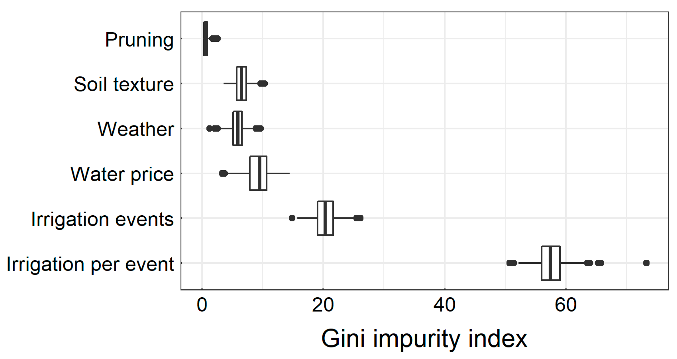
2.8. Decision Variable Importance
3. Case Study
3.1. Study Area
3.2. Argicultural Input and Water Cost
3.3. Crop Yield
3.4. Alternative Conditions and Strategies

| Soil Texture Class | ||
|---|---|---|
| Loamy Sand (LS) | 0.15 | 0.07 |
| Sandy Loam (SL) | 0.23 | 0.11 |
| Clay (Cl) | 0.36 | 0.22 |
3.5. Simple Multicriteria Approach
- The relative amount (in percentage) of the disposed water used during the irrigation compared to the full-scale irrigation in order to reach the field capacity (100%, 75%, 50%).
- The reduction in frequency (number of irrigation times) during the cultivation season compared to the number recommended for maximum crop yield (recommended n -1, recommended n-2).
- The profit from the farm. This is calculated by subtracting the costs of irrigation from the revenue from selling the crop.
3.6. Multicriteria Approach with Posterior Information
3.7. Multicriteria Fuzzy Approach
- Excellent application (Fuzzy Element 1).
- Good application (Fuzzy Element 2).
- Moderate application (Fuzzy Element 3).
3.8. Shortcomings of Probabilistic Approaches
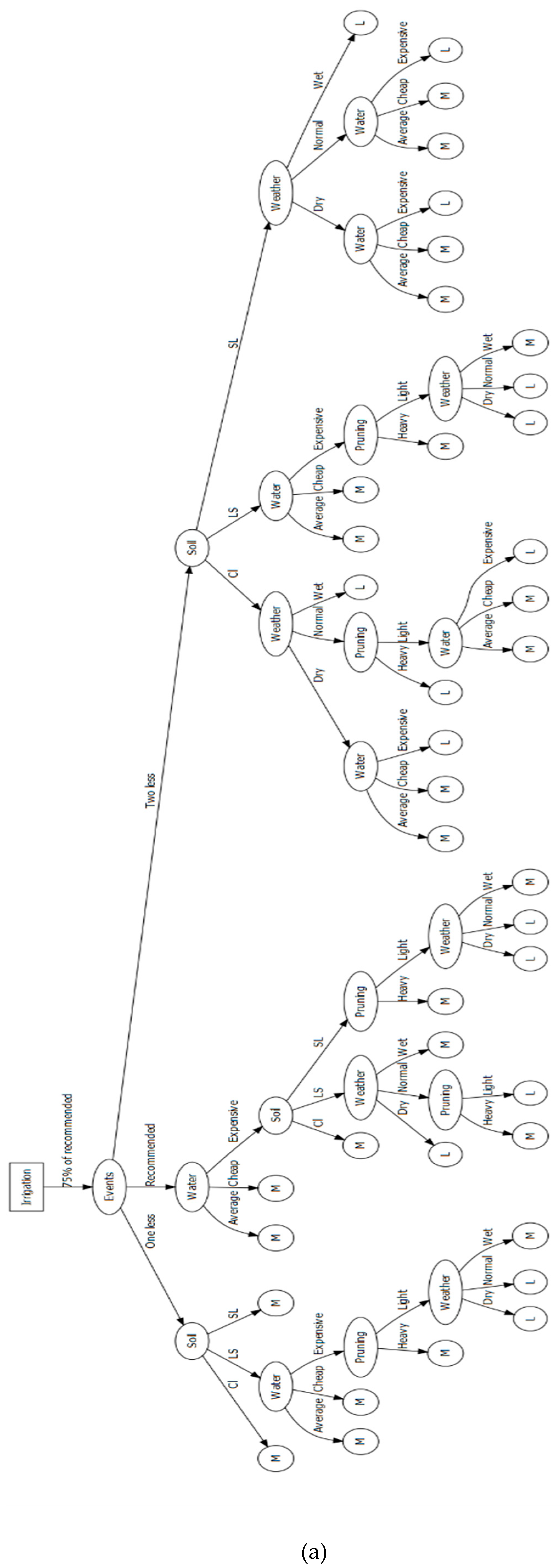
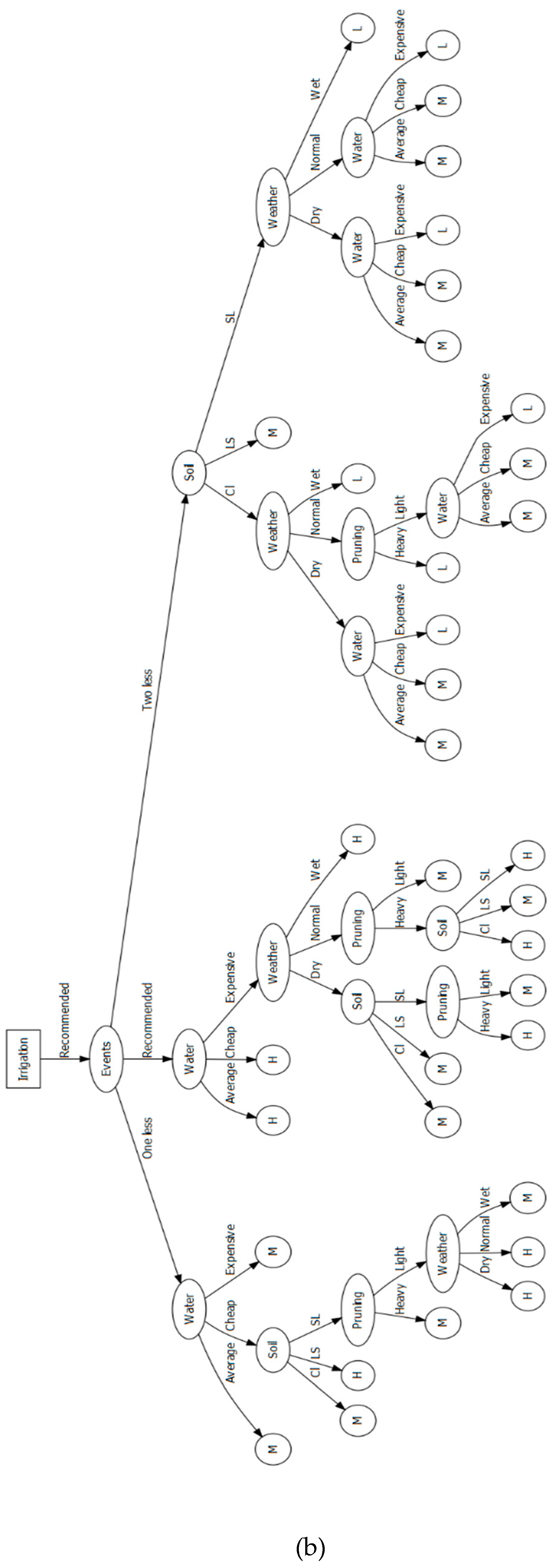
3.9. Decision Tree and the ID3 Algorithm
- Soil type. Possible soil types are loamy sand, sandy loam, and clay.
- Weather during cropping season. Wet, normal, and dry.
- Management practices. They are chosen to be: M1 heavy pruning and M2 light pruning. Tree pruning may bring down the total production, but it is a wise choice during a dry year (low in precipitation).
- The irrigation amount as a percentage of the recommended amount per irrigation event.
- The reduction in irrigation events related to the recommended.
4. Results and Discussion
4.1. Simple Multicriteria Approach
4.2. Multicriteria Approach with Posterior Information
4.3. Multicriteria Fuzzy Approach
4.4. Decision Tree and the ID3 Algorithm
4.5. Limitations
5. Conclusions
Author Contributions
Funding
Acknowledgments
Conflicts of Interest
References
- Aquastat, FAO’s Information System on Water and Agriculture, Food and Agriculture Organization (FAO) of the United Nation. Available online: http://www.fao.org/nr/water/aquastat (accessed on 5 December 2019).
- Brauman, K.A.; Siebert, S.; Foley, J.A. Improvements in crop water productivity increase water sustainability and food security a global analysis. Environ. Res. Lett. 2013, 8, 24030. [Google Scholar] [CrossRef]
- Cuevas, J.; Daliakopoulos, I.N.; del Moral, F.; Hueso, J.J.; Tsanis, I.K. A Review of Soil-Improving Cropping Systems for Soil Salinization. Agronomy 2019, 9, 295. [Google Scholar] [CrossRef]
- Ali, M.H.; Talukder, M.S.U. Increasing water productivity in crop production-A synthesis. Agric. Water Manag. 2008, 95, 1201–1213. [Google Scholar] [CrossRef]
- Fischer, G. Transforming the global food system. Nature 2018, 562, 501–502. [Google Scholar] [CrossRef]
- WWAP. World Water Development Report Volume 4: Managing Water under Uncertainty and Risk; United Nations Educational, Scientific and cultural Organization: Paris, France, 2012; Volume 1. [Google Scholar]
- Koutroulis, A.; Grillakis, M.; Daliakopoulos, I.; Tsanis, I.; Jacob, D. Cross sectoral impacts on water availability at +2 °C and +3 °C for east Mediterranean island states: The case of Crete. J. Hydrol. 2016, 532, 16–28. [Google Scholar] [CrossRef]
- Giannakis, E.; Bruggeman, A.; Djuma, H.; Kozyra, J.; Hammer, J. Water pricing and irrigation across Europe: Opportunities and constraints for adopting irrigation scheduling decision support systems. Water Sci. Technol. Water Supply 2016, 16, 245–252. [Google Scholar] [CrossRef]
- Labadie, J.W.; Sullivan, C.H. Computerized decision support systems for water managers. J. Water Resour. Plan. Manag. 1986, 112, 299–307. [Google Scholar] [CrossRef]
- Gurría, A. Sustainably managing water: Challenges and responses. Water Int. 2009, 34, 396–401. [Google Scholar] [CrossRef]
- Paredes, P.; Wei, Z.; Liu, Y.; Xu, D.; Xin, Y.; Zhang, B.; Pereira, L.S. Performance assessment of the FAO AquaCrop model for soil water, soil evaporation, biomass and yield of soybeans in North China Plain. Agric. Water Manag. 2015, 152, 57–71. [Google Scholar] [CrossRef]
- Steduto, P.; Hsiao, T.C.; Raes, D.; Fereres, E. AquaCrop-The FAO Crop Model to Simulate Yield Response to Water: I. Concepts and Underlying Principles. Agron. J. 2009, 101, 426–437. [Google Scholar] [CrossRef]
- Foster, T.; Brozović, N.; Butler, A.P.; Neale, C.M.U.; Raes, D.; Steduto, P.; Fereres, E.; Hsiao, T.C. AquaCrop-OS: An open source version of FAO’s crop water productivity model. Agric. Water Manag. 2017, 181, 18–22. [Google Scholar] [CrossRef]
- Mannini, P.; Genovesi, R.; Letterio, T. IRRINET: Large Scale DSS Application for On-farm Irrigation Scheduling. Procedia Environ. Sci. 2013, 19, 823–829. [Google Scholar] [CrossRef]
- Allen, R.G.; Pereira, L.S.; Raes, D.; Smith, M. Others Crop Evapotranspiration-Guidelines for Computing Crop Water Requirements-FAO Irrigation and Drainage Paper 56; FAO: Rome, Italy, 1998; Volume 300, p. 6541. [Google Scholar]
- Rinaldi, M.; He, Z. Decision Support Systems to Manage Irrigation in Agriculture. In Advances in Agronomy; Academic Press Inc.: Cambridge, MA, USA, 2014; Volume 123, pp. 229–279. [Google Scholar]
- Car, N.J. USING decision models to enable better irrigation Decision Support Systems. Comput. Electron. Agric. 2018, 152, 290–301. [Google Scholar] [CrossRef]
- Kahraman, C.; Kabak, Ö. Fuzzy statistical decision-making. In Studies in Fuzziness and Soft Computing; Springer: Cham, Sweitzerland, 2016; p. 343. [Google Scholar]
- Zimmermann, H.-J. Fuzzy Set Theory—And Its Applications; Springer: Dordrecht, Germany, 2001. [Google Scholar]
- Chernov, V.; Dorokhov, O.; Dorokhova, L.; Chubuk, V. Using fuzzy logic for solution of economic tasks: Two examples of decision making under uncertainty 85. ELIT-Econ. Lab. Transit. Res. 2013, 9, 85–100. [Google Scholar]
- Bates, J.H.T.; Young, M.P. Applying fuzzy logic to medical decision making in the intensive care unit. Am. J. Respir. Crit. Care Med. 2003, 167, 948–952. [Google Scholar] [CrossRef] [PubMed]
- Yao, J.F.F.; Yao, J.S. Fuzzy decision making for medical diagnosis based on fuzzy number and compositional rule of inference. Fuzzy Sets Syst. 2001, 120, 351–366. [Google Scholar] [CrossRef]
- Ross, T.J. Fuzzy Logic with Engineering Applications, 3rd ed.; Wiley: West Sussex, UK, 2010; p. 580. [Google Scholar]
- Christias, P. A comparative study on decision support approaches under uncertainty. In Business Information Systems Workshops; Abramowicz, W., Paschke, A., Eds.; BIS 2018. Lecture Notes in Business Information Processing; Springer: Cham, Switzerland, 2019; Volume 339, pp. 517–526. [Google Scholar]
- Bellman, R.E.; Zadeh, L.A. Decision-Making in a Fuzzy Environment. Manag. Sci. 1970, 17, 141–164. [Google Scholar] [CrossRef]
- Baghban, A.; Jalali, A.; Shafiee, M.; Ahmadi, M.H.; Chau, K. Developing an ANFIS-based swarm concept model for estimating the relative viscosity of nanofluids. Eng. Appl. Comput. Fluid Mech. 2019, 13, 26–39. [Google Scholar] [CrossRef]
- Shamshirband, S.; Rabczuk, T.; Chau, K.W. A Survey of Deep Learning Techniques: Application in Wind and Solar Energy Resources. IEEE Access 2019, 7, 164650–164666. [Google Scholar] [CrossRef]
- Najafi, B.; Faizollahzadeh Ardabili, S.; Shamshirband, S.; Chau, K.; Rabczuk, T. Application of ANNs, ANFIS and RSM to estimating and optimizing the parameters that affect the yield and cost of biodiesel production. Eng. Appl. Comput. Fluid Mech. 2018, 12, 611–624. [Google Scholar] [CrossRef]
- Ardabili, S.F.; Najafi, B.; Shamshirband, S.; Bidgoli, B.M.; Deo, R.C.; Chau, K.W. Computational intelligence approach formodeling hydrogen production: A review. Eng. Appl. Comput. Fluid Mech. 2018, 12, 438–458. [Google Scholar]
- Wang, W.C.; Xu, L.; Chau, K.W.; Xu, D. Yin-Yang firefly algorithm based on dimensionally Cauchy mutation. Expert Syst. Appl. 2020, 150, 113216. [Google Scholar] [CrossRef]
- Fotovatikhah, F.; Herrera, M.; Shamshirband, S.; Chau, K.W.; Ardabili, S.F.; Piran, M.J. Survey of computational intelligence as basis to big flood management: Challenges, research directions and future work. Eng. Appl. Comput. Fluid Mech. 2018, 12, 411–437. [Google Scholar] [CrossRef]
- Giusti, E.; Marsili-Libelli, S. A Fuzzy Decision Support System for irrigation and water conservation in agriculture. Environ. Model. Softw. 2015, 63, 73–86. [Google Scholar] [CrossRef]
- Li, M.; Sui, R.; Meng, Y.; Yan, H. A real-time fuzzy decision support system for alfalfa irrigation. Comput. Electron. Agric. 2019, 163, 104870. [Google Scholar] [CrossRef]
- Tsanis, I.K.; Koutroulis, A.G.; Daliakopoulos, I.N.; Jacob, D. Severe climate-induced water shortage and extremes in Crete. Clim. Chang. 2011, 106, 667–677. [Google Scholar] [CrossRef]
- Daliakopoulos, I.N.; Panagea, I.S.; Tsanis, I.K.; Grillakis, M.G.; Koutroulis, A.G.; Hessel, R.; Mayor, A.G.; Ritsema, C.J. Yield Response of Mediterranean Rangelands under a Changing Climate. Land Degrad. Dev. 2017, 28, 1962–1972. [Google Scholar] [CrossRef]
- Er-Raki, S.; Chehbouni, A.; Hoedjes, J.; Ezzahar, J.; Duchemin, B.; Jacob, F. Improvement of FAO-56 method for olive orchards through sequential assimilation of thermal infrared-based estimates of ET. Agric. Water Manag. 2008, 95, 309–321. [Google Scholar] [CrossRef]
- Allen, R.G.; Pruitt, W.O.; Wright, J.L.; Howell, T.A.; Ventura, F.; Snyder, R.; Itenfisu, D.; Steduto, P.; Berengena, J.; Yrisarry, J.B.; et al. A recommendation on standardized surface resistance for hourly calculation of reference ETo by the FAO56 Penman-Monteith method. Agric. Water Manag. 2006, 81, 1–22. [Google Scholar] [CrossRef]
- Blaney, H.F.; Criddle, W.D. Determining Consumptive Use and Irrigation Water Requirements; US Department of Agriculture: Washington, DC, USA, 1962.
- Kuslu, Y.; Sahin, U.; Tunc, T.; Kiziloglu, F.M. Determining water-yield relationship, water use efficiency, seasonal crop and pan coefficients for alfalfa in a semiarid region with high altitude. Bulg. J. Agric. Sci. 2010, 16, 482–492. [Google Scholar]
- Istanbulluoglu, A. Effects of irrigation regimes on yield and water productivity of safflower (Carthamus tinctorius L.) under Mediterranean climatic conditions. Agric. Water Manag. 2009, 96, 1792–1798. [Google Scholar] [CrossRef]
- Kipkorir, E.; Raes, D.; Massawe, B. Seasonal water production functions and yield response factors for maize and onion in Perkerra, Kenya. Agric. Water Manag. 2002, 56, 229–240. [Google Scholar] [CrossRef]
- Akhter, J.; Mahmood, K.; Tasneem, M.A.; Naqvi, M.H.; Malik, K.A. Comparative water-use efficiency of Sporobolus arabicus and Leptochloa fusca and its relation with carbon-isotope discrimination under semi-arid conditions. Plant Soil 2003, 249, 263–269. [Google Scholar] [CrossRef]
- Lovelli, S.; Perniola, M.; Ferrara, A.; Di Tommaso, T. Yield response factor to water (Ky) and water use efficiency of Carthamus tinctorius L. and Solanum melongena L. Agric. Water Manag. 2007, 92, 73–80. [Google Scholar] [CrossRef]
- Steduto, P.; Hsiao, T.C.; Fereres, E.; Raes, D. Crop Yield Response to Water; FAO: Rome, Italy, 2012. [Google Scholar]
- Moutonnet, P. Yield response factors of field crops to deficit irrigation. In Deficit Irrigation Practices. Water Reports 22; FAO: Rome, Italy, 2002; pp. 11–15. [Google Scholar]
- Popova, Z.; Eneva, S.; Pereira, L.S. Model Validation, Crop Coefficients and Yield Response Factors for Maize Irrigation Scheduling based on Long-term Experiments. Biosyst. Eng. 2006, 95, 139–149. [Google Scholar] [CrossRef]
- Orgaz, F.; Fereres, E. Riego. El Cultivo del Olivo; Barranco, D., Fernandez-Escobar, R., Rallo, L., Eds.; Ediciones Mundi-Prensa: Madrid, Spain, 2017; pp. 251–272. [Google Scholar]
- Allen, R.G.; Pereira, L.S. Estimating crop coefficients from fraction of ground cover and height. Irrig. Sci. 2009, 28, 17–34. [Google Scholar] [CrossRef]
- Rai, R.K.; Singh, V.P.; Upadhyay, A. Planning and Evaluation of Irrigation Projects: Methods and Implementation; Elsevier: Amsterdam, The Netherlands, 2017. [Google Scholar]
- Allen, R.G. Using the FAO-56 dual crop coefficient method over an irrigated region as part of an evapotranspiration intercomparison study. J. Hydrol. 2000, 229, 27–41. [Google Scholar] [CrossRef]
- Torres-Ruíz, J.M.; Fernández, J.E.; Girón, I.F.; Romero, R.; Jiménez-Bocanegra, J.A.; García Tejero, I.; Martín-Palomo, M.J. Determining evapotranspiration in an olive orchard in Southwest Spain. Acta Hortic. 2012, 949, 251–258. [Google Scholar] [CrossRef]
- Fereres, E.; Villalobos, F.J.; Orgaz, F.; Testi, L. Water requirements and irrigation scheduling in olive. Acta Hortic. 2011, 888, 31–40. [Google Scholar] [CrossRef]
- Stuart, M.; Ross, S.M. Introduction to Probability and Statistics for Engineers and Scientists. J. R. Stat. Soc. Ser. A 1988, 151, 381. [Google Scholar] [CrossRef][Green Version]
- Pownuk, A.; Kreinovich, V. Decision making under uncertainty. In Combining Interval, Probabilistic, and Other Types of Uncertainty in Engineering Applications. Studies in Computational Intelligence; Springer: Cham, Switzerland, 2018; Volume 773, pp. 157–190. [Google Scholar]
- Pirie, W.R.; Freund, J.E. Introduction to Probability. J. Am. Stat. Assoc. 1973, 68, 1028. [Google Scholar] [CrossRef]
- Bertsekas, D.P.; Tsitsiklis, J.N. Introduction to Probability, 2nd ed.; Athena Scientific: Nashua, NH, USA, 2008; Volume 1, pp. 18–43. [Google Scholar]
- Christias, P.; Mocanu, M. Enhancing bayes’ probabilistic decision support with a fuzzy approach. In Proceedings of the 2019 22nd International Conference on Control Systems and Computer Science, CSCS 2019, Bucharest, Romania, 28–30 May 2019. [Google Scholar]
- Alsolami, F.; Azad, M.; Chikalov, I.; Moshkov, M. Decision and Inhibitory Trees and Rules for Decision Tables with Many-Valued Decisions; Springer Nature Switzerland AG: Cham, Switzerland, 2020; Volume 156, pp. 17–36, 91–103. [Google Scholar]
- Hssina, B.; Merbouha, A.; Ezzikouri, H.; Erritali, M. A comparative study of decision tree ID3 and C4.5. Int. J. Adv. Comput. Sci. Appl. 2014, 4, 13–19. [Google Scholar] [CrossRef]
- Machine Learning: Complete Beginners Guide for Neural Networks, Algorithms, Random Forests and Decision Tress Made Simple; CreateSpace Independent Publishing: Scotts Valley, CA, USA, 2017.
- Altay, A.; Cinar, D. Fuzzy decision trees. Stud. Fuzziness Soft Comput. 2016, 343, 221–261. [Google Scholar]
- Di Prima, S.; Castellini, M.; Pirastru, M.; Keesstra, S. Soil Water Conservation: Dynamics and Impact. Water 2018, 10, 952. [Google Scholar] [CrossRef]
- Akkaş, E.; Akin, L.; Evren Çubukçu, H.; Artuner, H. Application of Decision Tree Algorithm for classification and identification of natural minerals using SEM-EDS. Comput. Geosci. 2015, 80, 38–48. [Google Scholar] [CrossRef]
- Wang, Y.Y.; Li, Y.B.; Rong, X.W. Improvement of ID3 algorithm based on simplified information entropy and coordination degree. In Proceedings of the Chinese Automation Congress, (CAC), IEEE, Jinan, China, 20–22 October 2017; pp. 1526–1550. [Google Scholar]
- Breiman, L. Technical Note: Some Properties of Splitting Criteria. Mach. Learn. 1996, 24, 41–47. [Google Scholar] [CrossRef]
- Cano, G.; Garcia-Rodriguez, J.; Garcia-Garcia, A.; Perez-Sanchez, H.; Benediktsson, J.A.; Thapa, A.; Barr, A. Automatic selection of molecular descriptors using random forest: Application to drug discovery. Expert Syst. Appl. 2017, 72, 151–159. [Google Scholar] [CrossRef]
- Friedman, J.; Hastie, T.; Tibshirani, R. The Elements of Statistical Learning: Data Mining, Inference, and Prediction, 2nd ed.; Springer: Cham, Switzerland, 2016. [Google Scholar]
- Bluemke, I.; Stepień, A. Selection of Metrics for the Defect Prediction; Springer: Cham, Switzerland, 2016; pp. 39–50. [Google Scholar]
- Koutroulis, A.G.; Vrohidou, A.-E.K.; Tsanis, I.K. Spatiotemporal Characteristics of Meteorological Drought for the Island of Crete. J. Hydrometeorol. 2011, 12, 206–226. [Google Scholar] [CrossRef]
- Tsanis, I.; Naoum, S. The effect of spatially distributed meteorological parameters on irrigation water demand assessment. Adv. Water Resour. 2003, 26, 311–324. [Google Scholar] [CrossRef]
- Naoum, S.; Tsanis, I.K. Temporal and spatial variation of annual rainfall on the island of Crete, Greece. Hydrol. Process. 2003, 17, 1899–1922. [Google Scholar] [CrossRef]
- Hellenic Statistical Authority. Annual Agricultural Statistics Report of the Hellenic Statistical Authority (ELSTAT). 2008. Available online: https://www.statistics.gr/en/hellenic_statistical_programme (accessed on 5 December 2019).
- Petousi, I.; Daliakopoulos, I.N.; Matsoukas, T.; Zotos, N.; Mavrogiannis, I.; Manios, T. DRIP: Development of an Advanced Precision Drip Irrigation System for Tree Crops. Terraenvision Abstr. 2018, 1, 2018–2022. [Google Scholar]
- Chartzoulakis, K.S. The use of saline water for irrigation of olives: Effects on growth, physiology, yield and oil quality. Acta Hortic. 2011, 888, 97–108. [Google Scholar] [CrossRef]
- Phogat, V.; Skewes, M.A.; Cox, J.W.; Sanderson, G.; Alam, J.; Šimůnek, J. Seasonal simulation of water, salinity and nitrate dynamics under drip irrigated mandarin (Citrus reticulata) and assessing management options for drainage and nitrate leaching. J. Hydrol. 2014, 513, 504–516. [Google Scholar] [CrossRef]
- Egea, G.; Diaz-Espejo, A.; Fernández, J.E. Soil moisture dynamics in a hedgerow olive orchard under well-watered and deficit irrigation regimes: Assessment, prediction and scenario analysis. Agric. Water Manag. 2016, 164, 197–211. [Google Scholar] [CrossRef]
- Agricultural News. Agricultural Input for Olive Trees and Olive Oil. 2019. Available online: https://www.news247.gr/agrotika/oi-eisroes-stin-elia-kai-to-elaiolado.6634173.html (accessed on 5 December 2019).
- OECD. Environmental Performance Reviews: Greece 2009; OECD Publications: Paris, France, 2009. [Google Scholar]
- Kapsalis, P.C.; Kritsotaki, M.A. 1st Revision of the River Basin Management Plan of the River Basin Districts of Crete (EL 13) Draft River Basin Management Plan, 3rd ed.; Hellenic Ministry of Environment and Energy: Athens, Greece, 2017.
- Stefanoudaki, E.; Chartzoulakis, K.; Koutsaftakis, A.; Kotsifaki, F. Effect of drought stress on qualitative characteristics of olive oil of cv Koroneiki. Grasas Aceites 2001, 52, 202–206. [Google Scholar] [CrossRef]
- Chartzoulakis, K.; Michelakis, N.; Tzompanakis, I. Effects of water amount and application date on yield and water utilization efficiency of “Koroneiki” olives under drip irrigation. Adv. Hortic. Sci. 1992, 6, 82–84. [Google Scholar]
- POOLred-Origin Price Information System for the Olive Oil Counting Market. Available online: http://www.poolred.com/ (accessed on 5 December 2019).
- Hellenic Ministry of Agriculture (HMU). Modernization of the Methodology of Calculating Irrigation Requirements Used in the Agricultural Technical Studies of Land Reclamation Projects and Adaptation to the Greek Conditions. Hellenic Ministry of Agriculture, Decision 120.344 11/2/1992. 1992. Available online: http://goodagro.org/docs/1992_Apofasi_Penman.pdf (accessed on 5 December 2019).
- Saxton, K.E.; Rawls, W.J. Soil Water Characteristic Estimates by Texture and Organic Matter for Hydrologic Solutions. Soil Sci. Soc. Am. J. 2006, 70, 1569–1578. [Google Scholar] [CrossRef]
- Gul, F.; Pesendorfer, W. Expected Uncertain Utility Theory. Econometrica 2014, 82, 1–39. [Google Scholar] [CrossRef]
- Fishburn, P.C. Utility Theory and Decision Theory. In Utility and Probability; Palgrave Macmillan: London, UK, 1990; pp. 303–312. [Google Scholar]
- Sadollah, A. Introductory Chapter: Which Membership Function is Appropriate in Fuzzy System? In Fuzzy Logic Based in Optimization Methods and Control Systems and its Applications; InTechOpen: London, UK, 2018. [Google Scholar] [CrossRef]
- Mcneil, B.; Pauker, S.G. Decision Analysis for Public Health: Principles and Illustrations. Ann. Rev. Public Health 1984, 5, 135–161. [Google Scholar] [CrossRef]
- Gravel, N.; Marchant, T.; Sen, A. Conditional expected utility criteria for decision making under ignorance or objective ambiguity. J. Math. Econ. 2018, 78, 79–95. [Google Scholar] [CrossRef]
- Luce, R.D.; Krantz, D.H. Conditional Expected Utility. Econometrica 1971, 39, 253. [Google Scholar] [CrossRef]
- Sheppard, C. Tree-Based Machine Learning Algorithms: Decision Trees, Random Forests, and Boosting; CreateSpace Independent Publishing Platform: Scotts Valley, CA, USA, 2017; p. 110. [Google Scholar]
- Subedi, A.; Chávez, J.L. Crop Evapotranspiration (ET) Estimation Models: A Review and Discussion of the Applicability and Limitations of ET Methods. J. Agric. Sci. 2015, 7, 50. [Google Scholar] [CrossRef]
- Li, M.; Guo, P.; Liu, X.; Huang, G.; Huo, Z. A decision-support system for cropland irrigation water management and agricultural non-point sources pollution control. Desalin. Water Treat. 2014, 52, 5106–5117. [Google Scholar] [CrossRef]
- Delgado, G.; Aranda, V.; Calero, J.; Sánchez-Marañón, M.; Serrano, J.M.; Sánchez, D.; Vila, M.A. Building a Fuzzy Logic Information Network and a Decision-Support System for Olive Cultivation in Andalusia [Spain]. Span. J. Agric. Res. 2008, 6, 252–263. [Google Scholar] [CrossRef]
- Katsigiannis, P.; Galanis, G.; Dimitrakos, A.; Tsakiridis, N.; Kalopesas, C.; Alexandridis, T.; Chouzouri, A.; Patakas, A.; Zalidis, G. Fusion of spatio-temporal UAV and proximal sensing data for an agricultural decision support system. In Proceedings of the Fourth International Conference on Remote Sensing and Geoinformation of the Environment (RSCy2016), Paphos, Cyprus, 12 August 2016; Volume 9688, p. 96881R. [Google Scholar]
- Daliakopoulos, I.N.; Grillakis, E.G.; Koutroulis, A.G.; Tsanis, I.K. Tree crown detection on multispectral VHR satellite imagery. Photogramm. Eng. Remote Sens. 2009, 75, 1201–1212. [Google Scholar] [CrossRef]
- Torres, I.; Sánchez, M.T.; Benlloch-González, M.; Pérez-Marín, D. Irrigation decision support based on leaf relative water content determination in olive grove using near infrared spectroscopy. Biosyst. Eng. 2019, 180, 50–58. [Google Scholar] [CrossRef]
- Moriana, A.; Girón, I.F.; Martín-Palomo, M.J.; Conejero, W.; Ortuño, M.F.; Torrecillas, A.; Moreno, F. New approach for olive trees irrigation scheduling using trunk diameter sensors. Agric. Water Manag. 2010, 97, 1822–1828. [Google Scholar] [CrossRef]
- Zaza, C.; Bimonte, S.; Faccilongo, N.; La Sala, P.; Contò, F.; Gallo, C. A new decision-support system for the historical analysis of integrated pest management activities on olive crops based on climatic data. Comput. Electron. Agric. 2018, 148, 237–249. [Google Scholar] [CrossRef]
- Carmona-Torres, C.; Parra-López, C.; Hinojosa-Rodríguez, A.; Sayadi, S. Farm-level multifunctionality associated with farming techniques in olive growing: An integrated modeling approach. Agric. Syst. 2014, 127, 97–114. [Google Scholar] [CrossRef]
- Liang, G. A Comparative Study of three Decision Tree Algorithms: ID3, Fuzzy ID3 and Probabilistic Fuzzy ID3; Erasmus University: Rotterdam, The Netherlands, 2005. [Google Scholar]


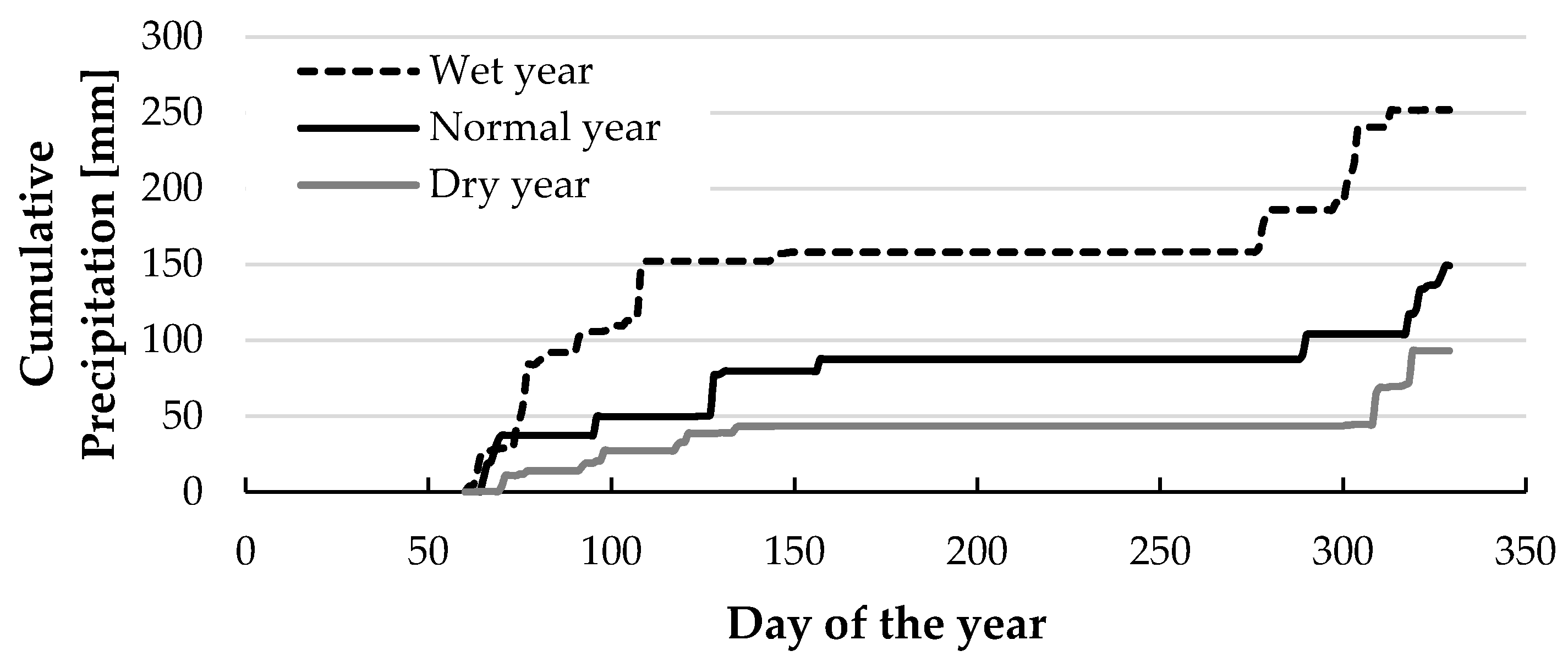
| Scenario | Total Precipitation * [mm] | Average Temperature [°C] | Total Reference Evapotranspiration [mm] |
|---|---|---|---|
| Wet year (W) | 251.9 | 20.7 | 1347.8 |
| Normal year (N) | 149.2 | 21.1 | 1361.3 |
| Dry year (D) | 93 | 21.4 | 1374.9 |
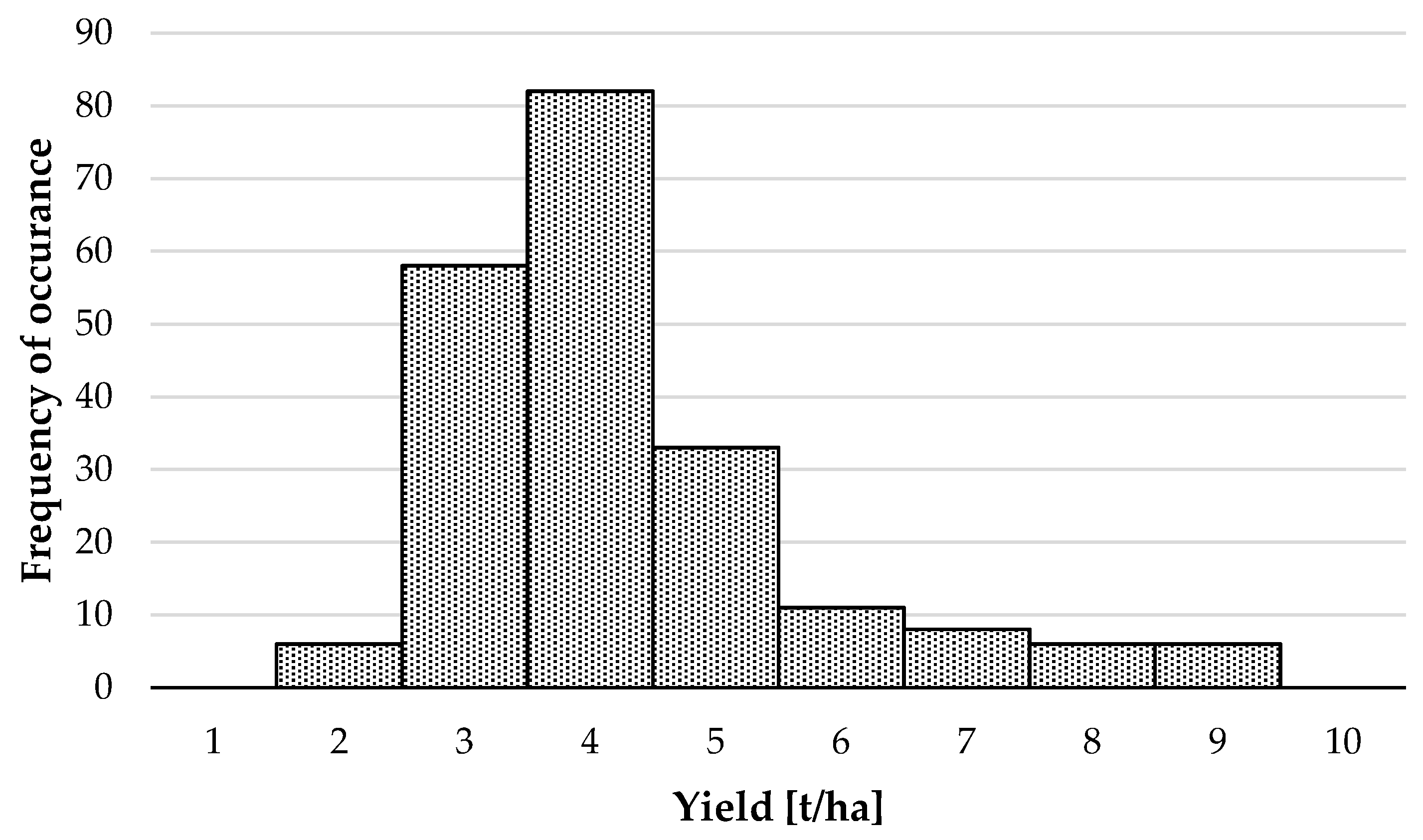
| Yield Class | Yield Range [t/ha] | |
|---|---|---|
| E | [1, 2] | 0.024 |
| D | [2, 4] | 0.667 |
| C | [4, 6] | 0.214 |
| B | [6, 8] | 0.067 |
| A | ≥8 | 0.029 |
| Scenario | Relative Irrigation | Reduction of Irrigation Events |
|---|---|---|
| 1 | 100% | 0 |
| 2 | 75% | 0 |
| 3 | 50% | 0 |
| 4 | 100% | 1 |
| 5 | 75% | 1 |
| 6 | 50% | 1 |
| 7 | 100% | 2 |
| 8 | 75% | 2 |
| 9 | 50% | 2 |
| Yield Label | |
|---|---|
| A | 0.029 |
| B | 0.067 |
| C | 0.214 |
| D | 0.667 |
| E | 0.024 |
| Precipitation | |
|---|---|
| Dry | 0.2 |
| Normal | 0.6 |
| Wet | 0.2 |
| Irrigation Strategy | 50%/n-2 | 50%/n-1 | 50%/n | 75%/n-2 | 75%/n-1 | 75%/n | 100%/n-2 | 100%/n-1 | 100%/n | |
|---|---|---|---|---|---|---|---|---|---|---|
| Profit | ||||||||||
| Low | 7 | 6 | 5 | 6 | 5 | 4 | 5 | 4 | 3 | |
| Medium | 8 | 7 | 6 | 7 | 6 | 5 | 6 | 7 | 4 | |
| High | 9 | 8 | 7 | 8 | 7 | 6 | 7 | 8 | 5 | |
| Profit Class | Total Score Range |
|---|---|
| Moderate | [1, 5) |
| Good | [5, 7] |
| Excellent | (7, 9] |
| Scenario → | 1 | 2 | 3 | 4 | 5 | 6 | 7 | 8 | 9 |
|---|---|---|---|---|---|---|---|---|---|
| 3.242 | 3.242 | 3.242 | 3.6341 | 4.8799 | 4.9742 | 4.0259 | 5.6277 | 6.5173 |
| Precipitation State | DRY | NORMAL | WET |
|---|---|---|---|
| 0.1667 | 0.1667 | 0.1296 | |
| 0.8333 | 0.8333 | 0.7037 | |
| 0 | 0 | 0.1667 | |
| 0 | 0 | 0 | |
| 0 | 0 | 0 |
| Scenario → | 1 | 2 | 3 | 4 | 5 | 6 | 7 | 8 | 9 |
|---|---|---|---|---|---|---|---|---|---|
| 8.3334 | 8.3334 | 8.3334 | 9.3409 | 12.5435 | 12.5435 | 10.3484 | 14.4659 | 16.7527 |
| Irrigation Strategy | 50%/n-2 | 50%/n-1 | 50%/n | 75%/n-2 | 75%/n-1 | 75%/n | 100%/n-2 | 100%/n-1 | 100%/n | |
|---|---|---|---|---|---|---|---|---|---|---|
| Profit | ||||||||||
| Low | μmod = 0 | μmod = 0 | μmod = 1/2 | μmod = 0 | μmod = 1/2 | μmod = 1 | μmod = 1/2 | μmod = 1 | μmod = 1 | |
| μgood = 1/2 | μgood = 1 | μgood = ½ | μgood = 1 | μgood = ½ | μgood = 0 | μgood = ½ | μgood = 0 | μgood = 0 | ||
| μexc = 1/2 | μexc = 0 | μexc = 0 | μexc = 0 | μexc = 0 | μexc = 0 | μexc = 0 | μexc = 0 | μexc = 0 | ||
| Medium | μmod = 0 | μmod = 0 | μmod = 0 | μmod = 0 | μmod = 0 | μmod = ½ | μmod = 0 | μmod = 0 | μmod = 1 | |
| μgood = 0 | μgood = ½ | μgood = 1 | μgood = ½ | μgood = 1 | μgood = ½ | μgood = 1 | μgood = ½ | μgood = 0 | ||
| μexc = 1 | μexc = 1/2 | μexc = 0 | μexc = 1/2 | μexc = 0 | μexc = 0 | μexc = 0 | μexc = 1/2 | μexc = 0 | ||
| High | μmod = 0 | μmod = 0 | μmod = 0 | μmod = 0 | μmod = 0 | μmod = 0 | μmod = 0 | μmod = 0 | μmod = ½ | |
| μgood = 0 | μgood = 0 | μgood = ½ | μgood = 0 | μgood = ½ | μgood = 1 | μgood = ½ | μgood = 0 | μgood = ½ | ||
| μexc = 1 | μexc = 1 | μexc = 1/2 | μexc = 1 | μexc = 1/2 | μexc = 0 | μexc = 1/2 | μexc = 1 | μexc = 0 | ||
| 0.3149 | 0.4444 | 0.2407 | 1 |
| Scenario → | 1 | 2 | 3 | 4 | 5 | 6 | 7 | 8 | 9 |
|---|---|---|---|---|---|---|---|---|---|
| Simple multicriteria | 3.2420 | 3.2420 | 3.2420 | 3.6341 | 4.8799 | 4.9742 | 4.0259 | 5.6277 | 6.5173 |
| Fuzzy | 3.0000 | 3.0000 | 3.0000 | 3.3627 | 4.5156 | 4.6029 | 3.7254 | 5.2077 | 6.0309 |
| Management Practice | Soil Type | Climate | Relative Irrigation | Trip Reduction Times | Irrigation/Trip (mm/ha) | Water Price (€/m3) | Profit (€/ha) | Profit |
|---|---|---|---|---|---|---|---|---|
| M1 | Cl | Normal | 100% | 1 | 134.4 | 0.05 | 1480.1 | Medium |
| M1 | SL | Wet | 50% | 2 | 129.6 | 0.05 | 281.8 | Low |
| M1 | SL | Normal | 50% | 2 | 72 | 0.13 | 679.5 | Low |
| M1 | SL | Dry | 50% | 0 | 43.2 | 0.13 | 579.5 | Low |
© 2020 by the authors. Licensee MDPI, Basel, Switzerland. This article is an open access article distributed under the terms and conditions of the Creative Commons Attribution (CC BY) license (http://creativecommons.org/licenses/by/4.0/).
Share and Cite
Christias, P.; Daliakopoulos, I.N.; Manios, T.; Mocanu, M. Comparison of Three Computational Approaches for Tree Crop Irrigation Decision Support. Mathematics 2020, 8, 717. https://doi.org/10.3390/math8050717
Christias P, Daliakopoulos IN, Manios T, Mocanu M. Comparison of Three Computational Approaches for Tree Crop Irrigation Decision Support. Mathematics. 2020; 8(5):717. https://doi.org/10.3390/math8050717
Chicago/Turabian StyleChristias, Panagiotis, Ioannis N. Daliakopoulos, Thrassyvoulos Manios, and Mariana Mocanu. 2020. "Comparison of Three Computational Approaches for Tree Crop Irrigation Decision Support" Mathematics 8, no. 5: 717. https://doi.org/10.3390/math8050717
APA StyleChristias, P., Daliakopoulos, I. N., Manios, T., & Mocanu, M. (2020). Comparison of Three Computational Approaches for Tree Crop Irrigation Decision Support. Mathematics, 8(5), 717. https://doi.org/10.3390/math8050717