Least-Squares Estimators of Drift Parameter for Discretely Observed Fractional Ornstein–Uhlenbeck Processes

Abstract

We introduce three new estimators of the drift parameter of a fractional Ornstein–Uhlenbeck process. These estimators are based on modifications of the least-squares procedure utilizing the explicit formula for the process and covariance structure of a fractional Brownian motion. We demonstrate their advantageous properties in the setting of discrete-time observations with fixed mesh size, where they outperform the existing estimators. Numerical experiments by Monte Carlo simulations are conducted to confirm and illustrate theoretical findings. New estimation techniques can improve calibration of models in the form of linear stochastic differential equations driven by a fractional Brownian motion, which are used in diverse fields such as biology, neuroscience, finance and many others.

1. Introduction

Stochastic models with fractional Brownian motion (fBm) as the noise source have attained increasing popularity recently. This is because fBm is a continuous Gaussian process, increments of which are positively, or negatively correlated if Hurst parameter $H>1/2$, or $H<1/2$, respectively. If $H=1/2$ fBm coincides with classical Brownian motion and its increments are independent. The ability of fBm to include memory into the noise process makes it possible to build more realistic models in such diverse fields as biology, neuroscience, hydrology, climatology, finance and many others. The interested reader may check monographs [1,2], or more recent paper [3] and the references therein for more information.

Let ${\{B_t^{\left(H\right)}\}}_{t\in [0,\infty )}$ be a fractional Brownian motion with Hurst parameter H defined on an appropriate probability space $\{\mathsf{\Omega },\mathcal{A},\mathrm{P}\}$. Fractional Ornstein–Uhlenbeck process (fOU) is the unique solution to the following linear stochastic differential equation

$$\begin{array}{c}\hfill \mathrm{d}{X}_t=-\lambda X_t\mathrm{d}t+\sigma \mathrm{d}{B}_t^{\left(H\right)},X_0=x_0\in \mathbb{R},t\ge 0,\end{array}$$

(1)

where $\lambda >0$ is a drift parameter (we consider ergodic case only) and $\sigma >0$ is a noise intensity (or volatility). Recall that solution to Equation (1) can be expressed by the exact analytical formula:

$$\begin{array}{c}\hfill X_t=e^{-\lambda t}{x}_0+\underset{0}{\overset{t}{\int }}{e}^{-\lambda (t-u)}\sigma \mathrm{d}{B}_u^{\left(H\right)}.\end{array}$$

(2)

A single realization of the random process ${\left\{X_t\left(\omega \right)\right\}}_{t\in [0,\infty )}$ for a particular $\omega \in \mathsf{\Omega }$ is the model for the single real-valued trajectory, part of which is observed. Two examples of such trajectories are given in Figure 1. We assume $H>1/2$ throughout this paper so that the fOU exhibits long-range dependence. For an example of application, see a neuronal model based on fOU described in the recent work [4].

The aim of this paper is to study the problem of estimating drift parameter $\lambda$ based on an observation of a single trajectory of a fOU in discrete time instants $t=0,h,\dots ,Nh$ with fixed mesh size $h>0$ and increasing time horizon $T=Nh\to \infty$ (long-span asymptotics). Estimating drift parameter of a fOU observed in continuous time has been considered in [5,6], where least-squares estimator (LSE) and ergodic-type estimator are studied. These have advantageous asymptotic properties, they are strongly consistent and, if $H\le 3/4$, also asymptotically normal. Ergodic-type estimator is easy to implement, but it has greater asymptotic variance compared to LSE, requires a priori knowledge of H and $\sigma$ and does not provide acceptable results for non-stationary processes with limited time horizon.

A straightforward discretization of the least-squares estimator for a fOU has been introduced and studied in [7] for $H>1/2$ and in [8] for $H<1/2$. For the precise formula, see (8). This estimator is consistent provided that both the time horizon $T=Nh\to \infty$ and the mesh size $h\to 0$ (mixed in-fill and long-span asymptotics). However, it is not consistent when h is fixed and $T\to \infty$. This has led us to construct and study LSE-type estimators that converge in this long-span setting.

An easy modification of the ergodic-type estimator to discrete-time setting with fixed time step was given in [9], see (10) for precise formula, and its strong consistency (assuming $H\ge 1/2$) and asymptotic normality (for $1/2\le H<3/4$) when $N\to \infty$ were proved, but with possibly incorrect technique (as pointed out in [10]). Correct proofs of asymptotic normality for $0<H\le 3/4$ and strong consistency for $0<H<1$ of this estimator were provided (in more general setup) in [10]. Note that the use of this discrete ergodic estimator requires the knowledge of parameter $\sigma$ (in contrast to the estimators of least-squares type introduced below). Other works related to estimating drift parameter for discretely observed fOU include [11,12,13], but this list is by no means complete.

This work contributes to the problem of estimating drift parameter of fOU by introducing three new LSE-type estimators: least-squares estimator from exact solution, asymptotic least-squares estimator and conditional least-squares estimator. These estimators are tailored to discrete-time observations with fixed time step. We provide proofs of their asymptotic properties and identify situations, in which these new estimators perform better than the already known ones. In particular, we eliminate the discretization error (the LSE from exact solution), construct strongly consistent estimators in the long-span regime without assuming in-fill condition (the asymptotic LSE and the conditional LSE), and eliminate the bias in the least-squares procedure caused by autocorrelation of the noise term (the conditional LSE). Especially the conditional LSE demonstrates outstanding performance in all studied scenarios. This suggests that the newly introduced (to our best knowledge) concept of conditioning in the least-squares procedure applied to the models with fractional noise provides a powerful framework for parameter estimation in this type of models. The proof of its strong consistency, presented within this paper, is rather non-trivial and may serve as a starting point for investigation of similar estimators in possibly different settings. A certain disadvantage of the conditional LSE is its complicated implementation (involving optimization procedure), which is in contrast to the other studied estimators.

Let us explain the strength of the conditional least-squares estimator in more detail. Comparison of the two trajectories in Figure 1 demonstrates the effect of different values of $\lambda$ on trajectories of fOU. In particular, it affects the speed of exponential decay in initial non-stationary phase and the variability in stationary phase. As we illustrate below, the discretized least-squares estimator, cf. (8), utilizes information about $\lambda$ from the exponential decay in initial phase, but is not capable to make use of the information contained in the variability in stationary phase. As a consequence, it is not consistent (in long-span setting). On the contrary, the ergodic-type estimator, cf. (10), is derived from the variance of the stationary distribution of the process. It works well for stationary processes (and is consistent), but leaves idle (and even worse, it is corrupted by) the observation of the process in its initial non-stationary phase. In result, neither of these estimators can efficiently estimate drift from long trajectories with far-from-stationary initial values. This gap is best filled with the conditional least-squares estimator, cf. (25), which effectively utilizes both information stored in non-stationary phase and in stationary phase of the observed process. This unique property is demonstrated in Results and Discussion, where the conditional LSE (denoted by ${\widehat{\lambda }}_5$) dominates the other estimators.

For the three newly introduced estimators the value of the Hurst parameter H is considered to be known a priori, whereas the knowledge of volatility parameter $\sigma$ is not required, which is an advantage of these methods. If H is not known, it can be estimated in advance by some of many methods, such as methods based on quadratic variations (cf. [14]), sample quantiles or trimmed means (cf. [15]), or on a wavelet transform (cf. [16]), to name just a few. Another useful works in this direction include simultaneous estimation of $\sigma$ and H using the powers of the second order variations (see [17], Chapter 3.3). The estimates of H (obtained independently from $\lambda$) can subsequently be used in the LSE-type estimators of lambda introduced below in a way similar to [18].

In Section 2, some elements of stochastic calculus with respect to fBm are recalled, stationary fOU is introduced and precise formulas for two existing drift estimators ${\widehat{\lambda }}_1$ and ${\widehat{\lambda }}_2$ are provided. Section 3 is devoted to construction of a new LSE type estimator (${\widehat{\lambda }}_3$) based on exact formula for fOU. A certain modification of ${\widehat{\lambda }}_3$ (denoted as ${\widehat{\lambda }}_4$), which ensures long-span consistency, is introduced in Section 4. In Section 5, we rewrite the linear model using conditional expectations to overcome the bias in LSE caused by autocorrelation of the noise. Least-squares method, applied to the conditional model with explicit formulas for conditional expectations, results in the conditional least-squares estimator (${\widehat{\lambda }}_5$). We prove strong consistency of this estimator. The actual performance of the newly introduced estimators ${\widehat{\lambda }}_3$,${\widehat{\lambda }}_4$ and ${\widehat{\lambda }}_5$ as well as its comparison to the already-known ${\widehat{\lambda }}_1$ and ${\widehat{\lambda }}_2$, is studied by Monte Carlo simulations in various scenarios and reported in Section 6. The simulated trajectories have been obtained in software R with YUIMA package (see [19]). Section 7 summarizes key points of the article and provides possible future extensions.

2. Preliminaries

For reader’s convenience we briefly review the basic concepts from theory of stochastic models with fractional noise in this section, including definition of fBm, Wiener integral of deterministic functions w.r.t. fBm and stationary fOU. This exposition follows [2,20]. For further reading, see also the monograph [1]. In the end of this section, we also recall formulas for discretized LSE and discrete ergodic estimator.

Fractional Brownian motion with Hurst parameter $H\in (0,1)$ is a centered (zero-mean) continuous Gaussian process ${\{B_t^{\left(H\right)}\}}_{t\in [0,\infty )}$ starting from zero ($B_0^{\left(H\right)}=0$ and having the following covariance structure

$$\begin{array}{c}\hfill \mathrm{E}\left(B_s^{\left(H\right)}{B}_t^{\left(H\right)}\right)=\frac{1}{2}\left(s^{2H}+t^{2H}-{|s-t|}^{2H}\right),s,t\ge 0.\end{array}$$

Note that for the purpose of construction of the stationary fOU, we need a two-sided fBm ${\{B_t^{\left(H\right)}\}}_{t\in \mathbb{R}}$ with t ranging over the whole $\mathbb{R}$. In this case we have

$$\begin{array}{c}\hfill \mathrm{E}\left(B_s^{\left(H\right)}{B}_t^{\left(H\right)}\right)=\frac{1}{2}\left({\left|s\right|}^{2H}+{\left|t\right|}^{2H}-{|s-t|}^{2H}\right),s,t\in \mathbb{R}.\end{array}$$

As a consequence, the increments of fBm are negatively correlated for $H<1/2$, independent for $H=1/2$ and positively correlated for $H>1/2$.

Consider a two-sided fBm with $H>1/2$ and define Wiener integral of a deterministic step function with respect to the fBm by formula

$$\begin{array}{c}\hfill \underset{\mathbb{R}}{\int }\sum _{i=1}^N{\alpha }_i{I}_{[t_i,t_{i+1}]}\left(s\right)\mathrm{d}{B}_s^{\left(H\right)}=\sum _{i=1}^N{\alpha }_i\left(B_{t_{i+1}}^{\left(H\right)}-B_{t_i}^{\left(H\right)}\right)\end{array}$$

for any positive integer N, real-valued coefficients ${\alpha }_1,\dots {\alpha }_N\in \mathbb{R}$ and a partition $-\infty <t_1\le \dots \le t_{N+1}<\infty$. This definition constitutes the following isometry for any pair of deterministic step functions f and g

$$\begin{array}{c}\hfill \mathrm{E}\left(\underset{\mathbb{R}}{\int }f\left(t\right)\mathrm{d}{B}_t^{\left(H\right)}\underset{\mathbb{R}}{\int }g\left(s\right)\mathrm{d}{B}_s^{\left(H\right)}\right)=\underset{{\mathbb{R}}^2}{\int \int }f\left(t\right)g\left(s\right)\phi (t,s)\mathrm{d}t\mathrm{d}s={\langle f,g\rangle }_H,\end{array}$$

(3)

where $\phi (t,s)={H(2H-1)|t-s|}^{2H-2}$. Using this isometry, we can extend the definition of the Wiener integral w.r.t. fBm to all elements of the space ${\mathcal{L}}_H^2\left(\mathbb{R}\right)$, defined as the completions of the space of deterministic step functions w.r.t. the scalar product ${\langle .,.\rangle }_H$ defined above. In result, the formula (3) holds true for any $f,g\in {\mathcal{L}}_H^2\left(\mathbb{R}\right)$, see also [21]. We will frequently use this formula in what follows, mainly to calculate the covariances of Wiener integrals.

Let ${\{B_t^{\left(H\right)}\}}_{t\in \mathbb{R}}$ be again a two-sided fBm with $H>1/2$. Define

$$\begin{array}{c}\hfill Z_0={\int }_{-\infty }^0{e}^{-\lambda (0-u)}\sigma \mathrm{d}{B}_u^{\left(H\right)},\end{array}$$

and denote by ${\left\{Z_t\right\}}_{t\in [0,\infty )}$ the solution to (1) with initial condition $Z_0$ in the sense that it satisfies

$$\begin{array}{c}\hfill \mathrm{d}{Z}_t=-\lambda Z_t\mathrm{d}t+\sigma \mathrm{d}{B}_t^{\left(H\right)}.\end{array}$$

This process is referred to as the stationary fOU and it can be expressed as

$$\begin{array}{c}\hfill Z_t={\int }_{-\infty }^t{e}^{-\lambda (t-u)}\sigma \mathrm{d}{B}_u^{\left(H\right)},t\ge 0.\end{array}$$

Note that the stationary fOU is an ergodic stationary Gaussian process (its autocorrelation function vanishes at infinity).

Consider now a stationary fOU ${\left\{Z_t\right\}}_{t\in [0,\infty )}$ observed at discrete time instants $t=0,h,2h,\cdots$. The ergodicity and the formula for the second moment of stationary fOU (see e.g., [20]) imply

$$\frac{1}{N}\sum _{n=0}^{N-1}{Z}_{nh}^2\stackrel{N\to \infty }{⟶}\mathrm{E}{Z}_0^2=\frac{{\sigma }^2}{{\lambda }^{2H}}H\mathsf{\Gamma }\left(2H\right)\mathrm{a}.\mathrm{s}.$$

(4)

Analogously,

$$\frac{1}{N}\sum _{n=0}^{N-1}{Z}_{nh}{Z}_{(n+1)h}\stackrel{N\to \infty }{⟶}\mathrm{E}{Z}_0{Z}_h\mathrm{a}.\mathrm{s}.,$$

(5)

and the expectation can be calculated using (3) and the change-of-variables formula

$$\begin{array}{cc}\hfill \mathrm{E}{Z}_0{Z}_h& =\mathrm{E}{Z}_0(e^{-\lambda h}{Z}_0+\underset{0}{\overset{h}{\int }}{e}^{-\lambda (h-u)}\sigma \mathrm{d}{B}_u^{\left(H\right)})\hfill \\ \hfill & =e^{-\lambda h}\frac{{\sigma }^2}{{\lambda }^{2H}}H\mathsf{\Gamma }\left(2H\right)+{\int }_0^h{\int }_{-\infty }^0{e}^{-\lambda (h-u)}{e}^{-\lambda (0-v)}{\sigma }^2{(u-v)}^{2H-2}H(2H-1)\mathrm{d}v\mathrm{d}u\hfill \\ \hfill & =e^{-\lambda h}\frac{{\sigma }^2}{{\lambda }^{2H}}H\mathsf{\Gamma }\left(2H\right)\left[1+\frac{2H-1}{\mathsf{\Gamma }\left(2H\right)}{\int }_0^{\lambda h}{\int }_{-\infty }^0{e}^{r+s}{(r-s)}^{2H-2}\mathrm{d}s\mathrm{d}r\right].\hfill \end{array}$$

(6)

The rest of this section is devoted to the two popular estimators of the drift parameter of fOU observed at discrete time instants described in Introduction—the discretized LSE and the discrete ergodic estimator. Start with the former. Consider a straightforward discrete approximation of the Equation (1):

$$\begin{array}{c}\hfill X_{n+h}-X_n\approx -\lambda X_{n}h+\sigma (B_{n+h}^{\left(H\right)}-B_n^{\left(H\right)}).\end{array}$$

(7)

Application of the standard least-squares procedure to the linear approximation above provides the discretized LSE studied in [7,8], which takes the form

$$\begin{array}{c}\hfill {\widehat{\lambda }}_1=-\frac{1}{h}\left(F_N-1\right),\end{array}$$

(8)

where h is the mesh size (time step) and

$$\begin{array}{c}\hfill F_N=\frac{{\displaystyle \sum _{n=0}^{N-1}}{X}_{nh}{X}_{(n+1)h}}{{\displaystyle \sum _{n=0}^{N-1}}{X}_{nh}^2},\end{array}$$

(9)

with $X_{nh}$ and $X_{(n+1)h}$ being the observations at adjacent time instants $t=nh$ and $t=(n+1)h$ respectively, of the process $X_t$ defined by (1) or (2). Note that having ${\widehat{\lambda }}_1$ expressed in term of $F_N$ simplifies its comparison with the estimators newly constructed in this paper. Recall that for consistency of ${\widehat{\lambda }}_1$ mixed in-fill and long-span asymptotics is required due to the approximation error in (7).

The discrete ergodic estimator is derived from asymptotic behavior of the (stationary) fOU. Recall the convergence in (4). Rearranging the terms provides an asymptotic formula for drift parameter $\lambda$ expressed in terms of the limit of the second sample moment of the stationary fOU. Substituting the stationary fOU by the observed fOU $X_h,X_{2h},\dots X_{Nh}$ in the asymptotic formula results in the discrete ergodic estimator:

$$\begin{array}{c}\hfill {\widehat{\lambda }}_2={\left(\frac{1}{N{\sigma }^{2}H\mathsf{\Gamma }\left(2H\right)}\sum _{i=1}^N{X}_{ih}\right)}^{-\frac{1}{2H}},\end{array}$$

(10)

which was studied in [9,10]. Recall that this estimator is strongly consistent in the long span regime (no in-fill condition needed), however, it heavily builds upon the asymptotic (stationary) behavior of the process and fails for processes with non-stationary initial phase (as illustrated by numerical experiments below).

3. Least-Squares Estimator from Exact Solution

Since the estimator ${\widehat{\lambda }}_1$ obtained from naive discretization of (1) provides reasonable approximations only for non-stationary solutions with short time horizon and small time step $h>0$ (as seen from numerical simulations below), we eliminate discretization error by considering exact analytical formula for $X_t$, see (2), and corresponding exact discrete formula for $X_{t+h}$,

$$\begin{array}{c}\hfill X_{t+h}=\beta X_t+{\xi }_t,\end{array}$$

(11)

where

$$\begin{array}{c}\hfill \beta =e^{-\lambda h},\mathrm{and}{\xi }_t=\underset{t}{\overset{t+h}{\int }}{e}^{-\lambda (t+h-u)}\sigma \mathrm{d}{B}_u^{\left(H\right)}.\end{array}$$

The least-squares estimator for $\beta$ w.r.t. linear model (11) is given by $\widehat{\beta }=F_N$, cf. (9), and the estimator for $\lambda$ can be defined as

$$\begin{array}{c}\hfill {\widehat{\lambda }}_3=-\frac{1}{h}log{F}_N.\end{array}$$

(12)

Numerical simulations show that ${\widehat{\lambda }}_3$ works well for non-stationary solutions and short time horizon ($T=10$ in simulations). The results for $H=0.6$ are presented in Figure 2. Simulation results for $H\in \{0.75,0.9\}$ are similar.

On the other hand, estimator ${\widehat{\lambda }}_3$ does not provide good results for observations with long time horizon ($T=1000$ in simulations) since ${\widehat{\lambda }}_3$ is not consistent if $N\to \infty$ and $h>0$ is fixed. The reason is that ${\xi }_t$ and $X_t$ in (11) are correlated. In fact, we can calculate the almost sure limit of ${\widehat{\lambda }}_3$ exactly. The limit is provided in Theorem 1. Its proof uses the following simple lemma (see [22]) to show the diminishing effect of the initial condition on limiting behaviour of sample averages. It is later used in the proof of Lemma 3 as well.

Lemma 1.

Consider real-valued sequences ${\left(a_n\right)}_{n=1}^{\infty }$ and ${\left(b_n\right)}_{n=1}^{\infty }$ such that

$$\begin{array}{c}\hfill \frac{1}{N}\sum _{n=1}^N\left|b_n\right|\stackrel{N\to \infty }{⟶}K<\infty ,\mathit{and}{a}_n\stackrel{n\to \infty }{⟶}0.\end{array}$$

Then $\frac{1}{N}{\sum }_{n=1}^N{a}_n{b}_n\stackrel{N\to \infty }{⟶}0$.

Theorem 1.

Let $h>0$ be fixed and define $f:(0,\infty )\to \mathbb{R}$ by

$$\begin{array}{c}\hfill f\left(x\right)=e^{-x}\left[1+\frac{2H-1}{\mathsf{\Gamma }\left(2H\right)}\underset{0}{\overset{x}{\int }}\left(\underset{-\infty }{\overset{0}{\int }}{e}^s{e}^r{(r-s)}^{2H-2}\mathrm{d}s\right)\mathrm{d}r\right].\end{array}$$

(13)

Then

$$\begin{array}{c}\hfill \underset{N\to \infty }{lim}{\widehat{\lambda }}_3=-\frac{1}{h}logf\left(\lambda h\right)almostsurely.\end{array}$$

(14)

In particular, $\underset{N\to \infty }{lim}{\widehat{\lambda }}_3<\lambda$.

Proof. 

Recall the asymptotic behavior of a stationary fOU described in formulas (4)–(6).

Since the effect of the initial condition vanishes at infinity, the limit behaviour of the non-stationary solution ${\left(X_{nh}\right)}_{n=0}^{\infty }$ is same. Indeed,

$$\begin{array}{c}\hfill \frac{1}{N}\sum _{n=0}^{N-1}{X}_{nh}{X}_{(n+1)h}-Z_{nh}{Z}_{(n+1)h}=\frac{1}{N}\sum _{n=0}^{N-1}(X_{nh}-Z_{nh})X_{(n+1)h}+\frac{1}{N}\sum _{n=0}^{N-1}(X_{(n+1)h}-Z_{(n+1)h})Z_{nh}.\end{array}$$

The convergence of the first summand to zero follows from the facts that

$$\begin{array}{c}\hfill (X_{nh}-Z_{nh})\stackrel{n\to \infty }{⟶}0\mathrm{a}.\mathrm{s}.,\frac{1}{N}\sum _{n=0}^{N-1}{X}_{(n+1)h}\stackrel{N\to \infty }{⟶}0\mathrm{a}.\mathrm{s}.\end{array}$$

and Lemma 1. Similar argument guarantees convergence of the second summand to zero as well. The convergence

$$\begin{array}{c}\hfill \frac{1}{N}\sum _{n=0}^{N-1}{X}_{nh}^2-Z_{nh}^2\stackrel{N\to \infty }{⟶}0\end{array}$$

can be shown correspondingly. In result, we obtain the almost sure convergence

$$\frac{{\displaystyle \sum _{n=0}^{N-1}}{X}_{nh}{X}_{(n+1)h}}{{\displaystyle \sum _{n=0}^{N-1}}{X}_{nh}^2}\stackrel{N\to \infty }{⟶}{e}^{-\lambda h}\left[1+\frac{2H-1}{\mathsf{\Gamma }\left(2H\right)}{\int }_0^{\lambda h}{\int }_{-\infty }^0{e}^{r+s}{(r-s)}^{2H-2}\mathrm{d}s\mathrm{d}r\right]=f\left(\lambda h\right).$$

(15)

The claim follows immediately from definition of ${\widehat{\lambda }}_3$. □

Remark 1.

Note that the convergence in (14) holds true also for $H=1/2$ (the double integral in f disappears) and for $H<1/2$ (utilizing the fact that a relation analogous to (3) is true even for $H<1/2$, if the two domains of integration are disjoint). Consequently

$$\begin{array}{c}\hfill \underset{N\to \infty }{lim}{\widehat{\lambda }}_3=-\frac{1}{h}logf\left(\lambda h\right)\left\{\begin{array}{cc}<\lambda ,\hfill & H>1/2,\hfill \\ =\lambda ,\hfill & H=1/2,\hfill \\ >\lambda ,\hfill & H<1/2.\hfill \end{array}\right.a.s.\end{array}$$

4. Asymptotic Least-Squares Estimator

Our goal in this section is modifying ${\widehat{\lambda }}_3$ so that it converges to $\lambda$ when $N\to \infty$ and $h>0$ is fixed. Combination of (12) and (14) yields $F_N\to f\left(\lambda h\right)$ a.s. Thus, we can define the asymptotic least-squares estimator ${\widehat{\lambda }}_4$ by relation $f\left(h{\widehat{\lambda }}_4\right)=F_N$. Since f is one-to-one (see below), the explicit formula for ${\widehat{\lambda }}_4$ reads

$$\begin{array}{c}\hfill {\widehat{\lambda }}_4=\frac{1}{h}{f}^{-1}\left(F_N\right).\end{array}$$

(16)

The following lemma justifies invertibility of f in the definition of ${\widehat{\lambda }}_4$.

Lemma 2.

In our setting $H>1/2$ the function f defined by (13) is strictly decreasing on $[0,\infty )$.

Proof. 

Calculate the derivative

$$\begin{array}{cc}\hfill f^{\prime }\left(x\right)& =-e^{-x}\left[1+\frac{2H-1}{\mathsf{\Gamma }\left(2H\right)}\underset{0}{\overset{x}{\int }}\left(\underset{-\infty }{\overset{0}{\int }}{e}^s{e}^r{(r-s)}^{2H-2}\mathrm{d}s\right)\mathrm{d}r\right]+e^{-x}\left[\frac{2H-1}{\mathsf{\Gamma }\left(2H\right)}\left(\underset{-\infty }{\overset{0}{\int }}{e}^s{e}^x{(x-s)}^{2H-2}\mathrm{d}s\right)\right]\hfill \\ \hfill & =e^{-x}\frac{2H-1}{\mathsf{\Gamma }\left(2H\right)}\left[\underset{-\infty }{\overset{0}{\int }}\left(e^s{e}^x{(x-s)}^{2H-2}-\underset{0}{\overset{x}{\int }}{e}^s{e}^r{(r-s)}^{2H-2}\mathrm{d}r\right)\mathrm{d}s-\frac{\mathsf{\Gamma }\left(2H\right)}{2H-1}\right].\hfill \end{array}$$

Continue with

$$\begin{array}{c}\hfill e^s{e}^x{(x-s)}^{2H-2}-\underset{0}{\overset{x}{\int }}{e}^s{e}^r{(r-s)}^{2H-2}\mathrm{d}r<{(x-s)}^{2H-2}{e}^s\left(e^x-\underset{0}{\overset{x}{\int }}{e}^r\mathrm{d}r\right)={(x-s)}^{2H-2}{e}^s<{(-s)}^{2H-2}{e}^s.\end{array}$$

Plug this estimate into the formula for $f^{\prime }\left(x\right)$ to see

$$\begin{array}{c}\hfill f^{\prime }\left(x\right)<e^{-x}\frac{2H-1}{\mathsf{\Gamma }\left(2H\right)}\left[\underset{-\infty }{\overset{0}{\int }}{(-s)}^{2H-2}{e}^s\mathrm{d}s-\frac{\mathsf{\Gamma }\left(2H\right)}{2H-1}\right]=e^{-x}\frac{2H-1}{\mathsf{\Gamma }\left(2H\right)}\left[\mathsf{\Gamma }(2H-1)-\mathsf{\Gamma }(2H-1)\right]=0.\end{array}$$

(17)

□

Remark 2.

Note that f is monotonous also for $H=1/2$, but it is not monotonous if $H<1/2$, which rules out the possibility to use estimator ${\widehat{\lambda }}_4$ in this singular case.

Theorem 2.

The asymptotic least-squares estimator ${\widehat{\lambda }}_4$ is strongly consistent, i.e.,

$$\begin{array}{c}\hfill \underset{N\to \infty }{lim}{\widehat{\lambda }}_4=\lambda a.s.\end{array}$$

Proof. 

Recall the definition of ${\widehat{\lambda }}_4$ in (16) and the limit in (15):

$$\begin{array}{c}\hfill F_N\stackrel{N\to \infty }{⟶}f\left(\lambda h\right)\mathrm{a}.\mathrm{s}.\end{array}$$

Further recall that $f:(0,\infty )\to (0,\infty )$ is differentiable with strictly negative derivative (see (17)). Thus, $f^{-1}$ is also differentiable with strictly negative derivative and this implies

$$\begin{array}{c}\hfill \underset{N\to \infty }{lim}{\widehat{\lambda }}_4=\underset{N\to \infty }{lim}\frac{1}{h}{f}^{-1}\left(F_N\right)=\frac{1}{h}{f}^{-1}\left(f\left(\lambda h\right)\right)=\lambda \mathrm{a}.\mathrm{s}.\end{array}$$

□

The strongly consistent estimator ${\widehat{\lambda }}_4$ works well for stationary solutions or observations with long time horizon (see Figure 3). Moreover it does not require explicit knowledge of $\sigma$ (in contrast to ${\widehat{\lambda }}_2$, which is also strictly consistent). On the other hand it does not provide adequate results for non-stationary solutions and short time horizon, since the correction function f reflects stationary behavior of the process (see Figure 4).

5. Conditional Least-Squares Estimator

Non-stationary trajectories with long time horizon contain a lot of information about $\lambda$, which is encoded mainly in two aspects: speed of decay in initial non-stationary phase and variance in stationary phase (see Figure 1). However, neither of the estimators ${\widehat{\lambda }}_1$,${\widehat{\lambda }}_2$, ${\widehat{\lambda }}_3$ or ${\widehat{\lambda }}_4$ can utilize all the information effectively. This motivates us to introduce another estimator. Recall that ${\widehat{\lambda }}_3$ fails to be consistent because of bias in LSE caused by the correlation between $X_t$ and ${\xi }_t$ in Equation (11). To eliminate the correlation between explanatory variable and noise term in the linear model, we switch to conditional expectations. Start from the following equation, which defines ${\eta }_t$:

$$\begin{array}{c}\hfill X_{t+h}=\mathrm{E}\left[X_{t+h}\right|X_t]+{\eta }_t={\mathrm{E}}_{\mathsf{\Lambda }=\lambda }\left[X_{t+h}\right|X_t]+{\eta }_t,\end{array}$$

(18)

where $\lambda$ is the true value of the unknown drift parameter and ${\mathrm{E}}_{\mathsf{\Lambda }}$ the (conditional) expectation with respect to the measure generated by the fOU ${\left\{X_t\right\}}_{t\in [0,\infty )}$ with drift value $\mathsf{\Lambda }$ and initial condition $x_0$. ($\mathsf{\Lambda }$ stands for an unknown throughout this section). In other words, ${\mathrm{E}}_{\mathsf{\Lambda }}\left[X_{t+h}\right|X_t]$ means the conditional expectation of $X_{t+h}$, conditioned by $X_t$, where the process X is given by (2) with drift $\lambda =\mathsf{\Lambda }$. Hence, ${\mathrm{E}}_{\lambda }$ has the same meaning as $\mathrm{E}$ in previous sections.

Obviously ${\mathrm{E}}_{\lambda }\left[{\eta }_t\right|X_t]=0$ and, consequently, $c_t(X_t,\mathsf{\Lambda })={\mathrm{E}}_{\mathsf{\Lambda }}\left[X_{t+h}\right|X_t]$ and ${\eta }_t$ are uncorrelated. Indeed,

$$\begin{array}{ccc}\hfill {\mathrm{E}}_{\lambda }\left((c_t(X_t,\mathsf{\Lambda })-{\mathrm{E}}_{\lambda }\left[c_t(X_t,\mathsf{\Lambda })\right]){\eta }_t\right)& =& {\mathrm{E}}_{\lambda }\left({\mathrm{E}}_{\lambda }\left[(c_t(X_t,\mathsf{\Lambda })-{\mathrm{E}}_{\lambda }\left[c_t(X_t,\mathsf{\Lambda })\right]){\eta }_t|X_t\right]\right)\hfill \\ & =& {\mathrm{E}}_{\lambda }\left((c_t(X_t,\mathsf{\Lambda })-{\mathrm{E}}_{\lambda }\left[c_t(X_t,\mathsf{\Lambda })\right]){\mathrm{E}}_{\lambda }\left[{\eta }_t|X_t\right]\right)=0.\hfill \end{array}$$

In result, we apply the least-squares technique to Equation (18), where $\lambda$ is to be estimated, i.e., we would like to minimize

$$\begin{array}{c}\hfill \underset{\mathsf{\Lambda }}{min}\sum _{n=0}^{N-1}{\left(X_{(n+1)h}-{\mathrm{E}}_{\mathsf{\Lambda }}\left[X_{(n+1)h}\right|X_{nh}]\right)}^2.\end{array}$$

To calculate $c_t(X_t,\mathsf{\Lambda })={\mathrm{E}}_{\mathsf{\Lambda }}\left[X_{t+h}\right|X_t]$ explicitly, use (11) and obtain

$$\begin{array}{c}\hfill {\mathrm{E}}_{\mathsf{\Lambda }}\left[X_{t+h}\right|X_t]=e^{-\mathsf{\Lambda }h}{X}_t+{\mathrm{E}}_{\mathsf{\Lambda }}\left[{\xi }_t\right|X_t].\end{array}$$

(19)

Note that random vector $({\xi }_t,X_t)$ has 2-dimensional normal distribution (dependent on parameter $\mathsf{\Lambda }$)

$$\begin{array}{c}\hfill \left[\begin{array}{c}{\xi }_t\\ X_t\end{array}\right]\sim \mathrm{N}\left(\left[\begin{array}{c}0\\ e^{-\mathsf{\Lambda }t}{x}_0\end{array}\right],\left[\begin{array}{cc}{\sigma }_{\xi }^2\left(\mathsf{\Lambda }\right)& {\sigma }_{\xi ,X}\left(\mathsf{\Lambda }\right)\\ {\sigma }_{\xi ,X}\left(\mathsf{\Lambda }\right)& {\sigma }_X^2\left(\mathsf{\Lambda }\right)\end{array}\right]\right),\end{array}$$

and we can use explicit expression for its conditional expectation to write

$$\begin{array}{c}\hfill {\mathrm{E}}_{\mathsf{\Lambda }}\left[{\xi }_t\right|X_t]=\left(X_t-e^{-\mathsf{\Lambda }t}{x}_0\right)\frac{{\sigma }_{\xi ,X}\left(\mathsf{\Lambda }\right)}{{\sigma }_X^2\left(\mathsf{\Lambda }\right)}.\end{array}$$

(20)

With respect to the exact formula for $X_t$ given by (2) and relation (3) we get

$$\begin{array}{ccc}\hfill {\sigma }_X^2\left(\mathsf{\Lambda }\right)& =& {\sigma }^{2}H(2H-1)\underset{0}{\overset{t}{\int }}\underset{0}{\overset{t}{\int }}{e}^{\mathsf{\Lambda }(u-t)}{e}^{\mathsf{\Lambda }(v-t)}{|u-v|}^{2H-2}\mathrm{d}v\mathrm{d}u\hfill \\ & =& \frac{{\sigma }^{2}H(2H-1)}{{\mathsf{\Lambda }}^{2H}}\underset{-\mathsf{\Lambda }t}{\overset{0}{\int }}\underset{-\mathsf{\Lambda }t}{\overset{0}{\int }}{e}^r{e}^s{|r-s|}^{2H-2}\mathrm{d}s\mathrm{d}r,\hfill \end{array}$$

where we used change-of-variable formula in the last step. Analogously

$$\begin{array}{ccc}\hfill {\sigma }_{\xi ,X}\left(\mathsf{\Lambda }\right)& =& {\sigma }^{2}H(2H-1)\underset{t}{\overset{t+h}{\int }}\left(\underset{0}{\overset{t}{\int }}{e}^{\mathsf{\Lambda }(u-t-h)}{e}^{\mathsf{\Lambda }(v-t)}{(u-v)}^{2H-2}\mathrm{d}v\right)\mathrm{d}u\hfill \\ & =& \frac{{\sigma }^{2}H(2H-1)}{{\mathsf{\Lambda }}^{2H}}{e}^{-\mathsf{\Lambda }h}\underset{0}{\overset{\mathsf{\Lambda }h}{\int }}\left(\underset{-\mathsf{\Lambda }t}{\overset{0}{\int }}{e}^r{e}^s{(r-s)}^{2H-2}\mathrm{d}s\right)\mathrm{d}r.\hfill \end{array}$$

Using the expressions for ${\sigma }_{\xi ,X}\left(\mathsf{\Lambda }\right)$ and ${\sigma }_X^2\left(\mathsf{\Lambda }\right)$ in (20) we obtain

$$\begin{array}{c}\hfill {\mathrm{E}}_{\mathsf{\Lambda }}\left[{\xi }_t\right|X_t]=\left(X_t-e^{-\mathsf{\Lambda }t}{x}_0\right)e^{-\mathsf{\Lambda }h}\frac{\underset{0}{\overset{\mathsf{\Lambda }h}{\int }}\left(\underset{-\mathsf{\Lambda }t}{\overset{0}{\int }}{e}^r{e}^s{(r-s)}^{2H-2}\mathrm{d}s\right)\mathrm{d}r}{\underset{-\mathsf{\Lambda }t}{\overset{0}{\int }}\underset{-\mathsf{\Lambda }t}{\overset{0}{\int }}{e}^r{e}^s{|r-s|}^{2H-2}\mathrm{d}s\mathrm{d}r}.\end{array}$$

(21)

Combining formula (21) with (19) yields

$${\mathrm{E}}_{\mathsf{\Lambda }}\left[X_{t+h}\right|X_t]=c_t(X_t,\mathsf{\Lambda })=X_t{A}_{\mathsf{\Lambda }t,\mathsf{\Lambda }h}-B_{\mathsf{\Lambda }t,\mathsf{\Lambda }h},$$

with

$$A_{\tau ,x}=e^{-x}\left(1+\frac{\underset{0}{\overset{x}{\int }}\left(\underset{-\tau }{\overset{0}{\int }}{e}^r{e}^s{(r-s)}^{2H-2}\mathrm{d}s\right)\mathrm{d}r}{\underset{-\tau }{\overset{0}{\int }}\underset{-\tau }{\overset{0}{\int }}{e}^r{e}^s{|r-s|}^{2H-2}\mathrm{d}s\mathrm{d}r}\right),$$

(22)

and

$$B_{\tau ,x}=e^{-\tau }{e}^{-x}{x}_0\frac{\underset{0}{\overset{x}{\int }}\left(\underset{-\tau }{\overset{0}{\int }}{e}^r{e}^s{(r-s)}^{2H-2}\mathrm{d}s\right)\mathrm{d}r}{\underset{-\tau }{\overset{0}{\int }}\underset{-\tau }{\overset{0}{\int }}{e}^r{e}^s{|r-s|}^{2H-2}\mathrm{d}s\mathrm{d}r}.$$

(23)

We can thus reformulate the Equation (18) for the observed process X as the following model (linear in $X_t$, but non-linear in $\mathsf{\Lambda }$):

$$\begin{array}{c}\hfill X_{t+h}={\left[X_t{A}_{\mathsf{\Lambda }t,\mathsf{\Lambda }h}-B_{\mathsf{\Lambda }t,\mathsf{\Lambda }h}\right]}_{\mathsf{\Lambda }=\lambda }+{\eta }_t.\end{array}$$

(24)

Now we aim to apply the least-squares method to the reformulated model to get the conditional least-squares estimator ${\widehat{\lambda }}_5$. To ensure the existence of global minima, we choose a closed interval $[{\mathsf{\Lambda }}_L,{\mathsf{\Lambda }}_U]\subset (0,\infty$) and define ${\widehat{\lambda }}_5$ as the minimizer of sum-of-squares function on this interval:

$$S_N\left({\widehat{\lambda }}_5\right)=\underset{\mathsf{\Lambda }\in [{\mathsf{\Lambda }}_L,{\mathsf{\Lambda }}_U]}{min}\left\{S_N\left(\mathsf{\Lambda }\right)\right\},$$

(25)

with criterion function $S_N$ defined as

$$S_N\left(\mathsf{\Lambda }\right)=\sum _{n=0}^{N-1}{\left[X_{(n+1)h}-\left(X_{nh}{A}_{\mathsf{\Lambda }nh,\mathsf{\Lambda }h}-B_{\mathsf{\Lambda }nh,\mathsf{\Lambda }h}\right)\right]}^2,$$

(26)

where we used (24) with $t=nh$.

Note that $S_N\left(\mathsf{\Lambda }\right)$ is continuous in $\mathsf{\Lambda }$ and therefore a minimum on the compact interval $[{\mathsf{\Lambda }}_L,{\mathsf{\Lambda }}_U]$ exists. Although model (24) is linear in $X_t$, the coefficients A and B depend on t and that complicates the numerical minimization of $S_N$.

Remark 3.

Let ${\left\{Z_t\right\}}_{t\in [0,\infty )}$ be the stationary solution to (1). Then

$$\begin{array}{c}\hfill {\mathrm{E}}_{\mathsf{\Lambda }}\left[Z_{t+h}\right|Z_t]=Z_t{A}_{\infty ,\mathsf{\Lambda }h}+0=Z_{t}f\left(\mathsf{\Lambda }h\right),\end{array}$$

where f is defined in (13) and $\mathsf{\Lambda }>0$ is arbitrary. Since the coefficient $f\left(\mathsf{\Lambda }h\right)$ does not depend on t, it is possible to calculate LSE for $f\left(\lambda h\right)$ explicitly and to construct the estimator of λ by applying $f^{-1}$. Such estimator coincides with ${\widehat{\lambda }}_4$ introduced in previous chapter. Thus ${\widehat{\lambda }}_4$ can be understood as the special case of conditional LSE for the stationary solution.

In order to prove strong consistency of the estimator ${\widehat{\lambda }}_5$ we need to verify uniform convergence of $(1/N)S_N\left(\mathsf{\Lambda }\right)$ to a function $S_{\infty }\left(\mathsf{\Lambda }\right)$ specified below. Let us start with the following proposition on uniform convergence of $A_{\tau ,x}$ and $B_{\tau ,x}$. This proposition will help us in the sequel to investigate limiting behaviour of the two terms $A_{\mathsf{\Lambda }nh,\mathsf{\Lambda }h}$ and $B_{\mathsf{\Lambda }nh,\mathsf{\Lambda }h}$ in the sum-of-squares function $S_N$.

Proposition 1.

Consider $A_{\tau ,x}$ and $B_{\tau ,x}$ defined by (22) and (23), and f defined by (13). Fix arbitrary $0<x_L<x_U<\infty$. Then

$$\underset{\tau \to \infty }{lim}\underset{x\in [x_L,x_U]}{sup}|A_{\tau ,x}-f\left(x\right)|=0,$$

(27)

and

$$\underset{\tau \to \infty }{lim}\underset{x\in [x_L,x_U]}{sup}\left|B_{\tau ,x}\right|=0.$$

(28)

Proof. 

In order to simplify the notation, denote

$$\begin{array}{c}\hfill I\left(\tau \right)=\underset{-\tau }{\overset{0}{\int }}\underset{-\tau }{\overset{0}{\int }}{e}^r{e}^s{|r-s|}^{2H-2}\mathrm{d}s\mathrm{d}r,J\left(\tau \right)=\underset{-\tau }{\overset{0}{\int }}{e}^s{(-s)}^{2H-2}\mathrm{d}s,\end{array}$$

and notice that

$$\begin{array}{c}\hfill I\left(\tau \right)\stackrel{\tau \to \infty }{⟶}\frac{\mathsf{\Gamma }\left(2H\right)}{2H-1}=\mathsf{\Gamma }(2H-1),J\left(\tau \right)\stackrel{\tau \to \infty }{⟶}\mathsf{\Gamma }(2H-1).\end{array}$$

Begin with (27):

$$\begin{array}{c}{\displaystyle \underset{x\in [x_L,x_U]}{sup}|A_{\tau ,x}-f\left(x\right)|}\hfill \\ =\underset{x\in [x_L,x_U]}{sup}{e}^{-x}\left|\frac{\underset{0}{\overset{x}{\int }}\left(\underset{-\tau }{\overset{0}{\int }}{e}^r{e}^s{(r-s)}^{2H-2}\mathrm{d}s\right)\mathrm{d}r}{\underset{-\tau }{\overset{0}{\int }}\underset{-\tau }{\overset{0}{\int }}{e}^r{e}^s{|r-s|}^{2H-2}\mathrm{d}s\mathrm{d}r}-\frac{\underset{0}{\overset{x}{\int }}\left(\underset{-\infty }{\overset{0}{\int }}{e}^s{e}^r{(r-s)}^{2H-2}\mathrm{d}s\right)\mathrm{d}r}{\mathsf{\Gamma }(2H-1)}\right|\hfill \\ \le e^{-x_L}\underset{x\in [x_L,x_U]}{sup}\left|\frac{\underset{0}{\overset{x}{\int }}\left(\underset{-\tau }{\overset{0}{\int }}{e}^r{e}^s{(r-s)}^{2H-2}\mathrm{d}s\right)\mathrm{d}r-\underset{0}{\overset{x}{\int }}\left(\underset{-\infty }{\overset{0}{\int }}{e}^s{e}^r{(r-s)}^{2H-2}\mathrm{d}s\right)\mathrm{d}r}{I\left(\tau \right)}\right|\hfill \\ +e^{-x_L}\underset{x\in [x_L,x_U]}{sup}\left|\frac{\left[\mathsf{\Gamma }(2H-1)-I\left(\tau \right)\right]\underset{0}{\overset{x}{\int }}\left(\underset{-\infty }{\overset{0}{\int }}{e}^s{e}^r{(r-s)}^{2H-2}\mathrm{d}s\right)\mathrm{d}r}{I\left(\tau \right)\mathsf{\Gamma }(2H-1)}\right|\hfill \\ \le \frac{e^{-x_L}}{I\left(\tau \right)}\underset{0}{\overset{x_U}{\int }}{e}^r\left(\underset{-\infty }{\overset{-\tau }{\int }}{e}^s{(r-s)}^{2H-2}\mathrm{d}s\right)\mathrm{d}r\hfill \\ +\frac{e^{-x_L}\left|\mathsf{\Gamma }(2H-1)-I\left(\tau \right)\right|}{I\left(\tau \right)\mathsf{\Gamma }(2H-1)}\underset{0}{\overset{x_U}{\int }}{e}^r\left(\underset{-\infty }{\overset{0}{\int }}{e}^s{(r-s)}^{2H-2}\mathrm{d}s\right)\mathrm{d}r\hfill \\ \le \frac{e^{-x_L}(\mathsf{\Gamma }(2H-1)-J\left(\tau \right))}{I\left(\tau \right)}\underset{0}{\overset{x_U}{\int }}{e}^r\mathrm{d}r+\frac{e^{-x_L}\left|\mathsf{\Gamma }(2H-1)-I\left(\tau \right)\right|}{I\left(\tau \right)}\underset{0}{\overset{x_U}{\int }}{e}^r\mathrm{d}r\stackrel{\tau \to \infty }{⟶}0.\hfill \end{array}$$

Similarly

$$\begin{array}{cc}\hfill & \underset{x\in [x_L,x_U]}{sup}\left|B_{\tau ,x}\right|\le e^{-\tau }{e}^{-x_L}{x}_0\frac{J\left(\tau \right)}{I\left(\tau \right)}\underset{0}{\overset{x_U}{\int }}{e}^r\mathrm{d}r\stackrel{\tau \to \infty }{⟶}0.\hfill \end{array}$$

□

Choose any $0<{\mathsf{\Lambda }}_L<{\mathsf{\Lambda }}_U<\infty$ and recall that $h>0$ is fixed. The uniform convergences in (27) and (28) imply the following convergences uniformly in $\mathsf{\Lambda }\in [{\mathsf{\Lambda }}_L,{\mathsf{\Lambda }}_U]$:

$$\underset{n\to \infty }{lim}\underset{\mathsf{\Lambda }\in [{\mathsf{\Lambda }}_L,{\mathsf{\Lambda }}_U]}{sup}|A_{\mathsf{\Lambda }nh,\mathsf{\Lambda }h}-f\left(\mathsf{\Lambda }h\right)|=0,$$

(29)

and

$$\underset{n\to \infty }{lim}\underset{\mathsf{\Lambda }\in [{\mathsf{\Lambda }}_L,{\mathsf{\Lambda }}_U]}{sup}\left|B_{\mathsf{\Lambda }nh,\mathsf{\Lambda }h}\right|=0,$$

(30)

respectively. Indeed, set $x_L={\mathsf{\Lambda }}_{L}h$ and $x_U={\mathsf{\Lambda }}_{U}h$ and fix any $\epsilon >0$. There is ${\tau }_0>0$ such that for any $\tau >{\tau }_0$,

$$\begin{array}{c}\hfill \underset{x\in [x_L,x_U]}{sup}|A_{\tau ,x}-f\left(x\right)|<\epsilon .\end{array}$$

If $n>\frac{{\tau }_0}{{\mathsf{\Lambda }}_{L}h}$, then $\mathsf{\Lambda }nh>{\tau }_0$ for any $\mathsf{\Lambda }\in [{\mathsf{\Lambda }}_L,{\mathsf{\Lambda }}_U]$. Consequently

$$\begin{array}{c}\hfill \underset{\mathsf{\Lambda }\in [{\mathsf{\Lambda }}_L,{\mathsf{\Lambda }}_U]}{sup}|A_{\mathsf{\Lambda }nh,\mathsf{\Lambda }h}-f\left(\mathsf{\Lambda }h\right)|<\epsilon ,\end{array}$$

which proves (29). The convergence in (30) can be shown analogously. These uniform convergences will be helpful in the proof of the following Lemma, which provides uniform convergence of $\frac{1}{N}{S}_N\left(\mathsf{\Lambda }\right)$ to a limiting function $S_{\infty }\left(\mathsf{\Lambda }\right)$. This uniform convergence is the key ingredient for the convergence of the minimizers ${\widehat{\lambda }}_5$.

Lemma 3.

Let f be defined by (13) and let $S_N\left(\mathsf{\Lambda }\right)$ be defined by (26), where ${\left\{X_t\right\}}_{t\in [0,\infty )}$ is the observed process with drift value λ. Denote

$$S_{\infty }\left(\mathsf{\Lambda }\right)=\frac{{\sigma }^2}{{\lambda }^{2H}}H\mathsf{\Gamma }\left(2H\right)\left(1-2f\left(\mathsf{\Lambda }h\right)f\left(\lambda h\right)+f^2\left(\mathsf{\Lambda }h\right)\right).$$

(31)

Then

$$\underset{N\to \infty }{lim}\underset{\mathsf{\Lambda }\in [{\mathsf{\Lambda }}_L,{\mathsf{\Lambda }}_U]}{sup}\left|\frac{1}{N}{S}_N\left(\mathsf{\Lambda }\right)-S_{\infty }\left(\mathsf{\Lambda }\right)\right|=0a.s.$$

(32)

Proof. 

First consider the stationary solution ${\left\{Z_t\right\}}_{t\in [0,\infty )}$ to (1) corresponding to drift value $\lambda$. Comparison of (6) with (13) yields

$$\begin{array}{c}\hfill {\mathrm{E}}_{\lambda }{Z}_0{Z}_h=f\left(\lambda h\right)\frac{{\sigma }^2}{{\lambda }^{2H}}H\mathsf{\Gamma }\left(2H\right).\end{array}$$

It enables us to write

$$\begin{array}{c}\hfill S_{\infty }\left(\mathsf{\Lambda }\right)={\mathrm{E}}_{\lambda }{Z}_0^2-2f\left(\mathsf{\Lambda }h\right){\mathrm{E}}_{\lambda }{Z}_0{Z}_h+f^2\left(\mathsf{\Lambda }h\right){\mathrm{E}}_{\lambda }{Z}_0^2\end{array}$$

for any $\mathsf{\Lambda }>0$, and, consequently

$$\begin{array}{cc}\hfill \frac{1}{N}{S}_N\left(\mathsf{\Lambda }\right)-S_{\infty }\left(\mathsf{\Lambda }\right)& =\left(\frac{1}{N}\sum _{n=0}^{N-1}{X}_{(n+1)h}^2-{\mathrm{E}}_{\lambda }{Z}_0^2\right)\hfill \\ \hfill & -2\left(\frac{1}{N}\sum _{n=0}^{N-1}{A}_{\mathsf{\Lambda }nh,\mathsf{\Lambda }h}{X}_{(n+1)h}{X}_{nh}-f\left(\mathsf{\Lambda }h\right){\mathrm{E}}_{\lambda }{Z}_0{Z}_h\right)\hfill \\ \hfill & +\left(\frac{1}{N}\sum _{n=0}^{N-1}{X}_{nh}^2{A}_{\mathsf{\Lambda }nh,\mathsf{\Lambda }h}^2-f^2\left(\mathsf{\Lambda }h\right){\mathrm{E}}_{\lambda }{Z}_0^2\right)\hfill \\ \hfill & +\left(\frac{1}{N}\sum _{n=0}^{N-1}{B}_{\mathsf{\Lambda }nh,\mathsf{\Lambda }h}\left(2X_{(n+1)h}-2A_{\mathsf{\Lambda }nh,\mathsf{\Lambda }h}{X}_{nh}+B_{\mathsf{\Lambda }nh,\mathsf{\Lambda }h}\right)\right).\hfill \end{array}$$

(33)

Recall that ${\left\{Z_t\right\}}_{t\in [0,\infty )}$ is ergodic and $|Z_t-X_t|$ vanishes at infinity. Using Lemma 1 in the same way as in the proof of Theorem 1 implies

$$\begin{array}{cc}\hfill & \underset{\mathsf{\Lambda }\in [{\mathsf{\Lambda }}_L,{\mathsf{\Lambda }}_U]}{sup}\left|\frac{1}{N}\sum _{n=0}^{N-1}{X}_{(n+1)h}^2-{\mathrm{E}}_{\lambda }{Z}_0^2\right|\stackrel{N\to \infty }{⟶}0\mathrm{a}.\mathrm{s}.\hfill \end{array}$$

For the second term, write

$$\begin{array}{c}{\displaystyle \underset{\mathsf{\Lambda }\in [{\mathsf{\Lambda }}_L,{\mathsf{\Lambda }}_U]}{sup}\left|\frac{1}{N}\sum _{n=0}^{N-1}{A}_{\mathsf{\Lambda }nh,\mathsf{\Lambda }h}{X}_{(n+1)h}{X}_{nh}-f\left(\mathsf{\Lambda }h\right){\mathrm{E}}_{\lambda }{Z}_0{Z}_h\right|}\hfill \\ \le \underset{\mathsf{\Lambda }\in [{\mathsf{\Lambda }}_L,{\mathsf{\Lambda }}_U]}{sup}|\frac{1}{N}\sum _{n=0}^{N-1}\left(A_{\mathsf{\Lambda }nh,\mathsf{\Lambda }h}-f\left(\mathsf{\Lambda }h\right)\right)X_{(n+1)h}{X}_{nh}\hfill \\ +\frac{1}{N}\sum _{n=0}^{N-1}f\left(\mathsf{\Lambda }h\right)\left(X_{(n+1)h}{X}_{nh}-{\mathrm{E}}_{\lambda }{Z}_0{Z}_h\right)|\hfill \\ \le \frac{1}{N}\sum _{n=0}^{N-1}\left(\underset{\mathsf{\Lambda }\in [{\mathsf{\Lambda }}_L,{\mathsf{\Lambda }}_U]}{sup}\left|A_{\mathsf{\Lambda }nh,\mathsf{\Lambda }h}-f\left(\mathsf{\Lambda }h\right)\right|\right)\left|X_{(n+1)h}{X}_{nh}\right|\hfill \\ +\left(\underset{\mathsf{\Lambda }\in [{\mathsf{\Lambda }}_L,{\mathsf{\Lambda }}_U]}{sup}\left|f\left(\mathsf{\Lambda }h\right)\right|\right)\left|\frac{1}{N}\sum _{n=0}^{N-1}{X}_{(n+1)h}{X}_{nh}-{\mathrm{E}}_{\lambda }{Z}_0{Z}_h\right|.\hfill \end{array}$$

Application of Lemma 1, the convergence in (29) and the continuity of f ensure the convergence with probability one of both summands to zero as $N\to \infty$.

The uniform convergence of the third term can be shown analogously:

$$\begin{array}{c}\hfill \underset{\mathsf{\Lambda }\in [{\mathsf{\Lambda }}_L,{\mathsf{\Lambda }}_U]}{sup}\left|\frac{1}{N}\sum _{n=0}^{N-1}{X}_{nh}^2{A}_{\mathsf{\Lambda }nh,\mathsf{\Lambda }h}^2-f^2\left(\mathsf{\Lambda }h\right){\mathrm{E}}_{\lambda }{Z}_0^2\right|\stackrel{N\to \infty }{⟶}0\mathrm{a}.\mathrm{s}.,\end{array}$$

where we use

$$\begin{array}{c}\hfill \underset{n\to \infty }{lim}\underset{\mathsf{\Lambda }\in [{\mathsf{\Lambda }}_L,{\mathsf{\Lambda }}_U]}{sup}|A_{\mathsf{\Lambda }nh,\mathsf{\Lambda }h}^2-f^2\left(\mathsf{\Lambda }h\right)|=0,\end{array}$$

which follows directly from (29) and the continuity of f.

The last term in (33) can be treated similarly:

$$\begin{array}{c}\hfill \underset{\mathsf{\Lambda }\in [{\mathsf{\Lambda }}_L,{\mathsf{\Lambda }}_U]}{sup}\left|\frac{1}{N}\sum _{n=0}^{N-1}{B}_{\mathsf{\Lambda }nh,\mathsf{\Lambda }h}\left(2X_{(n+1)h}-2A_{\mathsf{\Lambda }nh,\mathsf{\Lambda }h}{X}_{nh}+B_{\mathsf{\Lambda }nh,\mathsf{\Lambda }h}\right)\right|\le \frac{1}{N}\sum _{n=0}^{N-1}\left(\underset{\mathsf{\Lambda }\in [{\mathsf{\Lambda }}_L,{\mathsf{\Lambda }}_U]}{sup}\left|B_{\mathsf{\Lambda }nh,\mathsf{\Lambda }h}\right|\right)C_n,\end{array}$$

where

$$\begin{array}{ccc}{C}_n\hfill & =& 2|X_{(n+1)h}|+2\left(\underset{\mathsf{\Lambda }\in [{\mathsf{\Lambda }}_L,{\mathsf{\Lambda }}_U]}{sup}|A_{\mathsf{\Lambda }nh,\mathsf{\Lambda }h}-f\left(\mathsf{\Lambda }h\right)|\right)\left|X_{nh}\right|\hfill \\ & & +2\left(\underset{\mathsf{\Lambda }\in [{\mathsf{\Lambda }}_L,{\mathsf{\Lambda }}_U]}{sup}\left|f\left(\mathsf{\Lambda }h\right)\right|\right)\left|X_{nh}\right|+\left(\underset{\mathsf{\Lambda }\in [{\mathsf{\Lambda }}_L,{\mathsf{\Lambda }}_U]}{sup}\left|B_{\mathsf{\Lambda }nh,\mathsf{\Lambda }h}\right|\right).\hfill \end{array}$$

By (30)

$$\begin{array}{c}\hfill \underset{\mathsf{\Lambda }\in [{\mathsf{\Lambda }}_L,{\mathsf{\Lambda }}_U]}{sup}\left|B_{\mathsf{\Lambda }nh,\mathsf{\Lambda }h}\right|\stackrel{n\to \infty }{⟶}0,\end{array}$$

and

$$\begin{array}{c}\hfill \frac{1}{N}\sum _{n=0}^{N-1}{C}_n\stackrel{N\to \infty }{⟶}{\mathrm{E}}_{\lambda }\left|Z_0\right|\left(1+2\underset{\mathsf{\Lambda }\in [{\mathsf{\Lambda }}_L,{\mathsf{\Lambda }}_U]}{sup}\left|f\left(\mathsf{\Lambda }h\right)\right|\right)<\infty \mathrm{a}.\mathrm{s}.\end{array}$$

Lemma 1 concludes the proof:

$$\begin{array}{c}\hfill \frac{1}{N}\sum _{n=0}^{N-1}\left(\underset{\mathsf{\Lambda }\in [{\mathsf{\Lambda }}_L,{\mathsf{\Lambda }}_U]}{sup}\left|B_{\mathsf{\Lambda }nh,\mathsf{\Lambda }h}\right|\right)C_n\stackrel{N\to \infty }{⟶}0\mathrm{a}.\mathrm{s}.\end{array}$$

□

Previous considerations lead to the convergence of ${\widehat{\lambda }}_5$, being the minimizers of $\frac{1}{N}{S}_N\left(\mathsf{\Lambda }\right)$ to the minimizer of $S_{\infty }\left(\mathsf{\Lambda }\right)$. Next lemma ensures that this minimizer coincides with the true drift value $\lambda$.

Lemma 4.

$S_{\infty }$ defined by (31) is continuous on $(0,\infty )$ and λ is the unique minimizer of $S_{\infty }$, i.e.,

$$\begin{array}{c}\hfill S_{\infty }\left(\lambda \right)<S_{\infty }\left(\mathsf{\Lambda }\right)\forall \mathsf{\Lambda }>0,\mathsf{\Lambda }\ne \lambda .\end{array}$$

Proof. 

By definition

$$\begin{array}{ccc}{S}_{\infty }\left(\mathsf{\Lambda }\right)\hfill & =& \frac{{\sigma }^2}{{\lambda }^{2H}}H\mathsf{\Gamma }\left(2H\right)(1-2f\left(\mathsf{\Lambda }h\right)f\left(\lambda h\right)+f^2\left(\mathsf{\Lambda }h\right))\hfill \\ & =& \frac{{\sigma }^2}{{\lambda }^{2H}}H\mathsf{\Gamma }\left(2H\right)(1-f^2\left(\lambda h\right)+f^2\left(\lambda h\right)-2f\left(\mathsf{\Lambda }h\right)f\left(\lambda h\right)+f^2\left(\mathsf{\Lambda }h\right))\hfill \\ & =& \frac{{\sigma }^2}{{\lambda }^{2H}}H\mathsf{\Gamma }\left(2H\right)\left(1-f^2\left(\lambda h\right)+{[f\left(\lambda h\right)-f\left(\mathsf{\Lambda }h\right)]}^2\right).\hfill \end{array}$$

The claim follows immediately, because f is one-to-one (it is strictly decreasing).

Continuity of $S_{\infty }$ is a direct consequence of the continuity of f. □

Now we are in a position to prove the strong consistency of ${\widehat{\lambda }}_5$.

Theorem 3.

Consider bounds $0<{\mathsf{\Lambda }}_L<{\mathsf{\Lambda }}_U<\infty$ so that they cover the true drift λ of the observed solution ${\left\{X_t\right\}}_{t\in [0,\infty )}$ to Equation (1), i.e., $\lambda \in ({\mathsf{\Lambda }}_L,{\mathsf{\Lambda }}_U)$. Then ${\widehat{\lambda }}_5$ defined in (25) is strongly consistent, i.e.,

$$\begin{array}{c}\hfill {\widehat{\lambda }}_5\stackrel{N\to \infty }{⟶}\lambda a.s.\end{array}$$

Proof. 

The proof follows standard argumentation from nonlinear regression and utilizes Lemma 3 and Lemma 4. Choose $\epsilon >0$ sufficiently small so that $[{\mathsf{\Lambda }}_L,{\mathsf{\Lambda }}_U]\backslash (\lambda -\epsilon ,\lambda +\epsilon )\ne \varnothing$ and set

$$\begin{array}{c}\hfill \delta =min\{S_{\infty }\left(\mathsf{\Lambda }\right)-S_{\infty }\left(\lambda \right):\mathsf{\Lambda }\in [{\mathsf{\Lambda }}_L,{\mathsf{\Lambda }}_U]\backslash (\lambda -\epsilon ,\lambda +\epsilon )\}>0.\end{array}$$

Consider a set of full measure on which the uniform convergence (32) holds and take $N_0>0$ such that

$$\begin{array}{c}\hfill \underset{\mathsf{\Lambda }\in [{\mathsf{\Lambda }}_L,{\mathsf{\Lambda }}_U]}{sup}\left|\frac{1}{N}{S}_N\left(\mathsf{\Lambda }\right)-S_{\infty }\left(\mathsf{\Lambda }\right)\right|<\frac{\delta }{3}\forall N\ge N_0.\end{array}$$

Fix any $N\ge N_0$. Then for arbitrary $\mathsf{\Lambda }\in [{\mathsf{\Lambda }}_L,{\mathsf{\Lambda }}_U]\backslash (\lambda -\epsilon ,\lambda +\epsilon )$ we get

$$\begin{array}{c}\hfill \frac{1}{N}{S}_N\left(\lambda \right)<S_{\infty }\left(\lambda \right)+\frac{\delta }{3}<S_{\infty }\left(\mathsf{\Lambda }\right)-\frac{\delta }{3}<\frac{1}{N}{S}_N\left(\mathsf{\Lambda }\right).\end{array}$$

As ${\widehat{\lambda }}_5$ minimizes $S_N$, for all $N\ge N_0$ we have

$$\begin{array}{c}\hfill |{\widehat{\lambda }}_5-\lambda |<\epsilon .\end{array}$$

Since $\epsilon$ was arbitrary (if small enough), we obtain the convergence

$$\begin{array}{c}\hfill {\widehat{\lambda }}_5\stackrel{N\to \infty }{⟶}\lambda \end{array}$$

on a set of full measure. □

6. Results and Discussion

In

Table 1. Root mean square errors of the studied estimators calculated using 100 numerical simulations with $\lambda =1/2$.

${\mathit{x}}_0$	T	H	${\widehat{\mathit{\lambda }}}_1$	${\widehat{\mathit{\lambda }}}_2$	${\widehat{\mathit{\lambda }}}_3$	${\widehat{\mathit{\lambda }}}_4$	${\widehat{\mathit{\lambda }}}_5$
0	1000	0.6	0.216161	0.0364895	0.167108	0.0464931	0.0462385
0	1000	0.75	0.350571	0.0484904	0.33802	0.0637274	0.0643273
0	1000	0.9	0.444239	0.120954	0.442423	0.174213	0.170646
100	1000	0.6	0.158561	0.237689	0.0840923	0.125846	0.0297993
100	1000	0.75	0.244412	0.160116	0.205152	0.358587	0.0497393
100	1000	0.9	0.326662	0.105573	0.309256	1.17871	0.0454533
0	10	0.6	0.333834	0.513897	0.347278	0.539418	0.488992
0	10	0.75	0.439545	0.590848	0.438978	0.608744	0.552812
0	10	0.9	0.528586	0.841335	0.527932	0.840721	0.635887
100	10	0.6	0.0259539	0.49369	0.024092	0.441152	0.0277489
100	10	0.75	0.031949	0.480362	0.029853	1.53454	0.0411947
100	10	0.9	0.0398104	0.457155	0.0376366	4.54265	0.0291719

we present comparison of the root mean square errors (RMSE) of all considered estimators for $\lambda =0.5$ and several combinations of $x_0$, T and H. Estimators ${\widehat{\lambda }}_1$ and ${\widehat{\lambda }}_3$ demonstrate good performance in scenarios with far-from-zero initial ($x_0=100$) condition and short time horizon ($T=10$) This illustrates the fact that these estimators reflect mainly the speed of convergence to zero of the observed process in its initial phase. Increasing time horizon to $T=1000$ adds a stationary phase to the observed trajectories, which distorts the estimators ${\widehat{\lambda }}_1$ and ${\widehat{\lambda }}_3$.

Estimators ${\widehat{\lambda }}_2$ and ${\widehat{\lambda }}_4$ perform well in settings with stationary-like initial condition ($x_0=0$) and long time horizon ($T=1000$). This is because they are constructed from the stationary behavior of the process. Taking far-from-zero initial condition ruins these estimators, unless trajectory is very long.

The conditional LSE, ${\widehat{\lambda }}_5$, shows reasonable performance in all studied scenarios and it significantly outperforms the other estimators in scenario with far-from-stationary initial condition ($x_0=100$) and long time horizon ($T=1000$). This results from the unique ability of this estimator to reflect and utilize information about the drift from both non-stationary (decreasing) phase and stationary (oscillating) phase. This is also illustrated on Figure 5. On the other hand, evaluation of ${\widehat{\lambda }}_5$ is the most numerically demanding compared the other studied estimators.

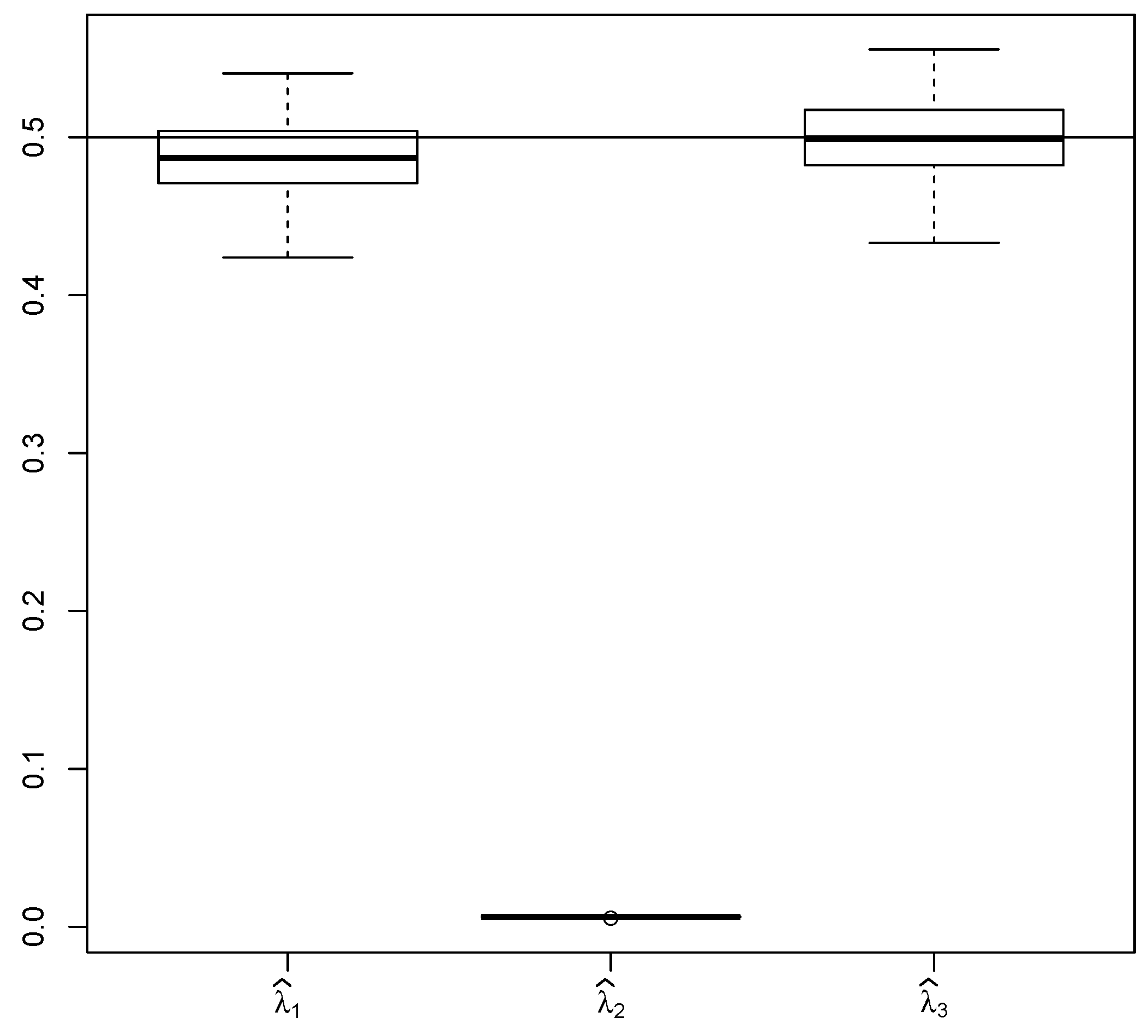
If $x_0=0$ and $T=10$, ${\widehat{\lambda }}_5$ shows greater RMSE than ${\widehat{\lambda }}_1$ and ${\widehat{\lambda }}_3$ in Table 1 due to $\lambda =1/2$ being relatively close to zero. This causes that ${\widehat{\lambda }}_1$ and ${\widehat{\lambda }}_3$ have smaller variance (although greater bias) compared to ${\widehat{\lambda }}_5$ (see Figure 6). In order to present this effect we have calculated RMSE for simulations in same scenario but with $\lambda =3/2$ (see

Table 2. Root mean square errors of the studied estimators calculated using 100 numerical simulations with $\lambda =3/2$.

${\mathit{x}}_0$	T	H	${\widehat{\mathit{\lambda }}}_1$	${\widehat{\mathit{\lambda }}}_2$	${\widehat{\mathit{\lambda }}}_3$	${\widehat{\mathit{\lambda }}}_4$	${\widehat{\mathit{\lambda }}}_5$
0	10	0.6	0.68946	0.641613	0.686183	0.761677	0.399386
0	10	0.75	1.11793	0.761793	1.10949	0.877707	0.457095
0	10	0.9	1.38463	1.21928	1.38299	1.52812	0.504919

). ${\widehat{\lambda }}_5$ provides smaller RMSE than the other estimators in this setting.

7. Conclusions

Three new estimators were defined and studied:

• The least-squares estimator from exact solution (${\widehat{\lambda }}_3$), which improves the popular discretized LSE (${\widehat{\lambda }}_1$) by eliminating the discretization error. It is easy to implement, since it can be calculated by a closed formula. However, it fails to be strongly consistent in long-span regime.
• The asymptotic least-squares estimator (${\widehat{\lambda }}_4$), which is a modification of ${\widehat{\lambda }}_3$ with respect to its asymptotic behavior. In result, ${\widehat{\lambda }}_4$ is strongly consistent in the long-span regime and behaves similarly to the well-established discrete ergodic estimator (${\widehat{\lambda }}_2$). The advantage of ${\widehat{\lambda }}_4$ is that it does not require a priori knowledge of the volatility $\sigma$. On the other hand, its implementation includes a root-finding numerical procedure.
• The conditional least-squares estimator (${\widehat{\lambda }}_5$), which eliminates the bias in the least-squares procedure by considering the conditional expectation of the response as the explanatory variable. The possibility to express the conditional expectation explicitly makes this approach feasible. This conditioning idea (which is new in the context of the models with fractional noise, to our best knowledge) provides exceptionally reliable estimator, which outperforms all the other studied estimators. We proved the strong consistency (in long-span regime) of this estimator. The implementation comprises solving an optimization problem.

These new estimating procedures can help practitioners or scientists from various fields to improve the calibration of their models based on available data with autocorrelated noise (these are typically observed/measured in discrete time instants) and, consequently, obtain more reliable conclusions from the calibrated models.

An interesting future extension would certainly be to explore the potential of the promising idea of the conditioning within least-squares procedure to more general models and settings (including d-dimensional fOU, fOU with $H<1/2$, non-linear drift, multiplicative noise, etc.).

References

1. Mishura, Y. Stochastic Calculus for Fractional Brownian Motion and Related Processes; Springer: Berlin/Heidelberg, Germany, 2008. [Google Scholar]
2. Biagini, F.; Hu, Y.; Øksendal, B.; Zhang, T. Stochastic Calculus for Fractional Brownian Motion and Applications; Springer: London, UK, 2008. [Google Scholar]
3. Abundo, M.; Pirozzi, E. On the Integral of the Fractional Brownian Motion and Some Pseudo-Fractional Gaussian Processes. Mathematics 2019, 7, 991. [Google Scholar] [CrossRef] [Green Version]
4. Ascione, G.; Mishura, Y.; Pirozzi, E. Fractional Ornstein–Uhlenbeck Process with Stochastic Forcing, and its Applications. Methodol. Comput. Appl. Probab. 2019. [Google Scholar] [CrossRef]
5. Hu, Y.; Nualart, D. Parameter estimation for fractional Ornstein–Uhlenbeck processes. Stat. Probab. Lett. 2010, 80, 1030–1038. [Google Scholar] [CrossRef] [Green Version]
6. Hu, Y.; Nualart, D.; Zhou, H. Parameter estimation for fractional Ornstein–Uhlenbeck processes of general Hurst parameter. Stat. Inference Stoch. Process. 2019, 22, 111–142. [Google Scholar] [CrossRef] [Green Version]
7. Es-Sebaiy, K. Berry-Esseen bounds for the least squares estimator for discretely observed fractional Ornstein–Uhlenbeck processes. Stat. Probab. Lett. 2013, 83, 2372–2385. [Google Scholar] [CrossRef] [Green Version]
8. Kubilius, K.; Mishura, Y.; Ralchenko, K.; Seleznjev, O. Consistency of the drift parameter estimator for the discretized fractional Ornstein–Uhlenbeck process with Hurst index H is an element of (0,1/2). Electron. J. Stat. 2015, 9, 1799–1825. [Google Scholar] [CrossRef]
9. Hu, Y.; Song, J. Parameter estimation for fractional Ornstein–Uhlenbeck processes with discrete observations. In Malliavin Calculus and Stochastic Analysis; Springer: Boston, MA, USA, 2013; Volume 34, pp. 427–442. [Google Scholar] [CrossRef] [Green Version]
10. Es-Sebaiy, K.; Viens, F. Optimal rates for parameter estimation of stationary Gaussian processes. Stoch. Process. Their. Appl. 2019, 129, 3018–3054. [Google Scholar] [CrossRef] [Green Version]
11. Azmoodeh, E.; Viitasaari, L. Parameter estimation based on discrete observations of fractional Ornstein–Uhlenbeck process of the second kind. Stat. Inference Stoch. Process. 2015, 18, 205–227. [Google Scholar] [CrossRef] [Green Version]
12. Neuenkirch, A.; Tindel, S. A least square-type procedure for parameter estimation in stochastic differential equations with additive fractional noise. Stat. Inference Stoch. Process. 2014, 17, 99–120. [Google Scholar] [CrossRef] [Green Version]
13. Xiao, W.; Zhang, W.; Xu, W. Parameter estimation for fractional Ornstein–Uhlenbeck processes at discrete observation. Appl. Math. Model. 2011, 35, 4196–4207. [Google Scholar] [CrossRef]
14. Istas, J.; Lang, G. Quadratic variations and estimation of the local Hölder index of a Gaussian process. Annales de l’I.H.P. Probabilités et Statistiques 1997, 33, 407–436. [Google Scholar] [CrossRef] [Green Version]
15. Coeurjolly, J. Hurst exponent estimation of locally self-similar Gaussian processes using sample quantiles. Ann. Stat. 2008, 36, 1404–1434. [Google Scholar] [CrossRef]
16. Rosenbaum, M. Estimation of the volatility persistence in a discretely observed diffusion model. Stoch. Process. Their. Appl. 2008, 118, 1434–1462. [Google Scholar] [CrossRef]
17. Berzin, C.; Latour, A.; León, J. Inference on the Hurst Parameter and Variance of Diffusions Driven by Fractional Brownian Motion; Springer International Publishing: Cham, Switzerland, 2014. [Google Scholar]
18. Brouste, A.; Iacus, S. Parameter estimation for the discretely observed fractional Ornstein–Uhlenbeck process and the Yuima R package. Comput. Stat. 2013, 28, 1529–1547. [Google Scholar] [CrossRef] [Green Version]
19. Brouste, A.; Fukasawa, M.; Hino, H.; Iacus, S.; Kamatani, K.; Koike, Y.; Masuda, H.; Nomura, R.; Ogihara, T.; Shimuzu, Y.; et al. The YUIMA Project: A Computational Framework for Simulation and Inference of Stochastic Differential Equations. J. Stat. Softw. 2014, 4, 1–51. [Google Scholar] [CrossRef]
20. Kubilius, K.; Mishura, Y.; Ralchenko, K. Parameter Estimation in Fractional Diffusion Models; Springer International Publishing AG: Cham, Switzerland, 2017. [Google Scholar]
21. Pipiras, V.; Taqqu, M. Integration questions related to fractional Brownian motion. Probab. Theory Relat. Fields 2000, 118, 251–291. [Google Scholar] [CrossRef]
22. Kříž, P.; Maslowski, B. Central limit theorems and minimum-contrast estimators for linear stochastic evolution equations. Stochastics 2019, 91, 1109–1140. [Google Scholar] [CrossRef] [Green Version]
Figure 1. Two single trajectories of fOU with different values of λ, where σ = 2, x0 = 20, T = 20, H = 0.6.
Mathematics 08 00716 g001
Figure 2. Comparison of λ ^ 1 , λ ^ 2 and λ ^ 3 for 100 trajectories, where H = 0.6 , x 0 = 100 , T = 10 , h = 0.1 , σ = 2 ; the horizontal line shows the true value of the estimated parameter λ = 0.5 .
Mathematics 08 00716 g002
Figure 3. Comparison of λ ^ 1 , λ ^ 2 , λ ^ 3 and λ ^ 4 for 100 trajectories, where H = 0.6 , x 0 = 0 , T = 1000 , h = 1 , σ = 2 ; the horizontal line shows the true value of the estimated parameter λ = 0.5 .
Mathematics 08 00716 g003
Figure 4. Comparison of λ ^ 1 , λ ^ 2 , λ ^ 3 and λ ^ 4 for 100 trajectories, where H = 0.6 , x 0 = 100 , T = 10 , h = 0.1 , σ = 2 ; the horizontal line shows the true value of the estimated parameter λ = 0.5 .
Mathematics 08 00716 g004
Figure 5. Comparison of λ ^ 1 , λ ^ 2 , λ ^ 3 , λ ^ 4 and λ ^ 5 for 100 trajectories, where H = 0.75 , x 0 = 100 , T = 1000 , h = 1 , σ = 2 ; the horizontal line shows the true value of the estimated parameter λ = 0.5 .
Mathematics 08 00716 g005
Figure 6. Comparison of λ ^ 1 , λ ^ 2 , λ ^ 3 , λ ^ 4 and λ ^ 5 for 100 trajectories, where H = 0.6 , x 0 = 0 , T = 10 , h = 0.1 , σ = 2 ; the horizontal line shows the true value of the estimated parameter λ = 0.5 .
Mathematics 08 00716 g006