Article

The VIF and MSE in Raise Regression

by
Román Salmerón Gómez
1,
Ainara Rodríguez Sánchez
2,
Catalina García García
1,* and
José García Pérez
3
1
Department of Quantitative Methods for Economics and Business, University of Granada, 18010 Granada, Spain
2
Department of Economic Theory and History, University of Granada, 18010 Granada, Spain
3
Department of Economy and Company, University of Almería, 04120 Almería, Spain
*
Author to whom correspondence should be addressed.
Mathematics 2020, 8(4), 605; https://doi.org/10.3390/math8040605
Submission received: 1 April 2020 / Accepted: 13 April 2020 / Published: 16 April 2020
(This article belongs to the Special Issue Quantitative Methods for Economics and Finance)

Abstract

:
The raise regression has been proposed as an alternative to ordinary least squares estimation when a model presents collinearity. In order to analyze whether the problem has been mitigated, it is necessary to develop measures to detect collinearity after the application of the raise regression. This paper extends the concept of the variance inflation factor to be applied in a raise regression. The relevance of this extension is that it can be applied to determine the raising factor which allows an optimal application of this technique. The mean square error is also calculated since the raise regression provides a biased estimator. The results are illustrated by two empirical examples where the application of the raise estimator is compared to the application of the ridge and Lasso estimators that are commonly applied to estimate models with multicollinearity as an alternative to ordinary least squares.

1. Introduction

In the last fifty years, different methods have been developed to avoid the instability of estimates derived from collinearity (see, for example, Kiers and Smilde [1]). Some of these methods can be grouped within a general denomination known as penalized regression.
In general terms, the penalized regression parts from the linear model (with p variables and n observations), Y = X β + u , and obtains the regularization of the estimated parameters, minimizing the following objective function:
( Y X β ) t ( Y X β ) + P ( β ) ,
where P ( β ) is a penalty term that can take different forms. One of the most common penalty terms is the bridge penalty term ([2,3]) is given by
P ( β ) = λ j = 1 p β j α , α > 0 ,
where λ is a tuning parameter. Note that the ridge ([4]) and the Lasso ([5]) regressions are obtained when α = 2 and α = 1 , respectively. Penalties have also been called soft thresholding ([6,7]).
These methods are applied not only for the treatment of multicollinearity but also for the selection of variables (see, for example, Dupuis and Victoria-Feser [8], Li and Yang [9] Liu et al. [10], or Uematsu and Tanaka [11]), which is a crucial issue in many areas of science when the number of variables exceeds the sample size. Zou and Hastie [12] proposed elastic net regularization by using the penalty terms λ 1 and λ 2 that combine the Lasso and ridge regressions:
P ( β ) = λ 1 j = 1 p β j + λ 2 j = 1 p β j 2 .
Thus, the Lasso regression usually selects one of the regressors from among all those that are highly correlated, while the elastic net regression selects several of them. In the words of Tutz and Ulbricht [13] “the elastic net catches all the big fish”, meaning that it selects the whole group.
From a different point of view, other authors have also presented different techniques and methods well suited for dealing with the collinearity problems: continuum regression ([14]), least angle regression ([15]), generalized maximum entropy ([16,17,18]), the principal component analysis (PCA) regression ([19,20]), the principal correlation components estimator ([21]), penalized splines ([22]), partial least squares (PLS) regression ([23,24]), or the surrogate estimator focused on the solution of the normal equations presented by Jensen and Ramirez [25].
Focusing on collinearity, the ridge regression is one of the more commonly applied methodologies and it is estimated by the following expression:
β ^ ( K ) = X t X + K · I 1 X t Y
where I is the identity matrix with adequate dimensions and K is the ridge factor (ordinary least squares (OLS) estimators are obtained when K = 0 ). Although ridge regression has been widely applied, it presents some problems with current practice in the presence of multicollinearity and the estimators derived from the penalty come into these same problems whenever n > p :
  • In relation to the calculation of the variance inflation factors (VIF), measures that quantify the degree of multicollinearity existing in a model from the coefficient of determination of the regression between the independent variables (for more details, see Section 2), García et al. [26] showed that the application of the original data when working with the ridge estimate leads to non-monotone VIF values by considering the VIF as a function of the penalty term. Logically, the Lasso and the elastic net regression inherit this property.
  • By following Marquardt [27]: “The least squares objective function is mathematically independent of the scaling of the predictor variables (while the objective function in ridge regression is mathematically dependent on the scaling of the predictor variables)”. That is to say, the penalized objective function will bring problems derived from the standardization of the variables. This fact has to be taken into account both for obtaining the estimators of the regressors and for the application of measures that detect if the collinearity has been mitigated. Other penalized regressions (such as Lasso and elastic net regressions) are not scale invariant and hence yield different results depending on the predictor scaling used.
  • Some of the properties of the OLS estimator that are deduced from the normal equations are not verified by the ridge estimator and, among others, the estimated values for the endogenous variable are not orthogonal to the residuals. As a result, the following decomposition is verified
    i = 1 n ( Y i Y ¯ ) 2 = i = 1 n ( Y ^ i ( K ) Y ¯ ) 2 + i = 1 n e i ( K ) 2 + 2 i = 1 n ( Y ^ i ( K ) Y ¯ ) · e i ( K ) .
    When the OLS estimators are obtained ( K = 0 ), the third term is null. However, this term is not null when K is not zero. Consequently, the relationship T S S ( K ) = E S S ( K ) + R S S ( K ) is not satisfied in ridge regression, and the definition of the coefficient of determination may not be suitable. This fact not only limits the analysis of the goodness of fit but also affects the global significance since the critical coefficient of determination is also questioned. Rodríguez et al. [28] showed that the estimators obtained from the penalties mentioned above inherit the problem of the ridge regression in relation to the goodness of fit.
In order to overcome these problems, this paper is focused on the raise regression (García et al. [29] and Salmerón et al. [30]) based on the treatment of collinearity from a geometrical point of view. It consists in separating the independent variables by using the residuals (weighted by the raising factor) of the auxiliary regression traditionally used to obtain the VIF. Salmerón et al. [30] showed that the raise regression presents better conditions than ridge regression and, more recently, García et al. [31] showed, among other questions, that the ridge regression is a particular case of the raise regression.
This paper presents the extension of the VIF to the raise regression showing that, although García et al. [31] showed that the application of the raise regression guarantees a diminishing of the VIF, it is not guaranteed that its value is lower the threshold traditionally established as troubling. Thus, it will be concluded that an unique application of the raise regression does not guarantee the mitigation of the multicollinearity. Consequently, this extension complements the results presented by García et al. [31] and determines, on the one hand, whether it is necessary to apply a successive raise regression (see García et al. [31] for more details) and, on the other hand, the most adequate variable for raising and the most optimal value for the raising factor in order to guarantee the mitigation of the multicollinearity.
On the other hand, the transformation of variables is common when strong collinearity exists in a linear model. The transformation to unit length (see Belsley et al. [32]) or standardization (see Marquardt [27]) is typical. Although the VIF is invariant to these transformations when it is calculated after estimation by OLS (see García et al. [26]), it is not guaranteed either in the case of the raise regression or in ridge regression as showed by García et al. [26]. The analysis of this fact is one of the goals of this paper.
Finally, since the raise estimator is biased, it is interesting to calculate its mean square error (MSE). It is studied whether the MSE of the raise regression is less than the one obtained by OLS. In this case, this study could be used to select an adequate raising factor similar to what is proposed by Hoerl et al. [33] in the case of the ridge regression. Note that estimators with MSE less than the one from OLS estimators are traditionally preferred (see, for example, Stein [34], James and Stein [35], Hoerl and Kennard [4], Ohtani [36], or Hubert et al. [37]). In addition, this measure allows us to conclude whether the raise regression is preferable, in terms of MSE, to other alternative techniques.
The structure of the paper is as follows: Section 2 briefly describes the VIF and the raise regression, and Section 3 extends the VIF to this methodology. Some desirable properties of the VIF are analyzed, and its asymptotic behavior is studied. It is also concluded that the VIF is invariant to data transformation. Section 4 calculates the MSE of the raise estimator, showing that there is a minimum value that is less than the MSE of the OLS estimator. Section 5 illustrates the contribution of this paper with two numerical examples. Finally, Section 6 summarizes the main conclusions of this paper.

2. Preliminaries

2.1. Variance Inflation Factor

The following model for p independent variables and n observations is considered:
Y = β 1 + β 2 X 2 + + β i X i + + β p X p + u = X β + u ,
where Y is a vector n × 1 that contains the observations of the dependent variable, X = [ 1 X 2 X i X p ] (with 1 being a vector of ones with dimension n × 1 ) is a matrix with order n × p that contains (by columns) the observations of the independent variables, β is a vector p × 1 that contains the coefficients of the independent variables, and u is a vector n × 1 that represents the random disturbance that is supposed to be spherical ( E [ u ] = 0 and V a r ( u ) = σ 2 I , where 0 is a vector with zeros with dimension n × 1 and I the identity matrix with adequate dimensions, in this case p × p ).
Given the model in Equation (2), the variance inflation factor (VIF) is obtained as follows:
V I F ( k ) = 1 1 R k 2 , k = 2 , , p ,
where R k 2 is the coefficient of determination of the regression of the variable X k as a function of the rest of the independent variables of the model in Equation (2):
X k = α 1 + α 2 X 2 + + α k 1 X k 1 + α k + 1 X k + 1 + + α p X p + v = X k α + v ,
where X k corresponds to the matrix X after the elimination of the column k (variable X k ).
If the variable X k has no linear relationship (i.e., is orthogonal) with the rest of the independent variables, the coefficient of determination will be zero ( R k 2 = 0 ) and the V I F ( k ) = 1 . As the linear relationship increases, the coefficient of determination ( R k 2 ) and consequently V I F ( k ) will also increase. Thus, the higher the VIF associated with the variable X k , the greater the linear relationship between this variable and the rest of the independent variables in the model in Equation (2). It is considered that the collinearity is troubling for values of VIF higher than 10. Note that the VIF ignores the role of the constant term (see, for example, Salmerón et al. [38] or Salmerón et al. [39]), and consequently, this extension will be useful when the multicollinearity is essential; that is to say, when there is a linear relationship between at least two independent variables of the model of regression without considering the constant term (see, for example, Marquandt and Snee [40] for the definitions of essential and nonessential multicollinearity).

2.2. Raise Regression

Raise regression, presented by García et al. [29] and more developed further by Salmerón et al. [30], uses the residuals of the model in Equation (4), e k , to raise the variable k as X ˜ k = X k + λ e k with λ 0 (called the raising factor) and to verify that e k t X k = 0 , where 0 is a vector of zeros with adequate dimensions. In that case, the raise regression consists in the estimation by OLS of the following model:
Y = β 1 ( λ ) + β 2 ( λ ) X 2 + + β k ( λ ) X ˜ k + + β p ( λ ) X p + u ˜ = X ˜ β ( λ ) + u ˜ ,
where X ˜ = [ 1 X 2 X ˜ k X p ] = [ X k X ˜ k ] . García et al. [29] showed (Theorem 3.3) that this technique does not alter the global characteristics of the initial model. That is to say, the models in Equations (2) and (5) have the same coefficient of determination and experimental statistics for the global significance test.
Figure 1 illustrates the raise regression for two independent variables being geometrically separated by using the residuals weighted by the raising factor λ . Thus, the selection of an adequate value for λ is essential, analogously to what occurs with the ridge factor K. A preliminary proposal about how to select the raising factor in a model with two independent standardized variables can be found in García et al. [41]. Other recently published papers introduce and highlight the various advantages of raise estimators for statistical analysis: Salmerón et al. [30] presented the raise regression for p = 3 standardized variables and showed that it presents better properties than the ridge regression and that the individual inference of the raised variable is not altered, García et al. [31] showed that it is guaranteed that all the VIFs associated with the model in Equation (5) diminish but that it is not possible to quantify the decrease, García and Ramírez [42] presented the successive raise regression, and García et al. [31] showed, among other questions, that ridge regression is a particular case of raise regression.
The following section presents the extension of the VIF to be applied after the estimation by raise regression since it will be interesting whether, after the raising of one independent variable, the VIF falls below 10. It will be also analyzed when a successive raise regression can be recommendable (see García and Ramírez [42]).

3. VIF in Raise Regression

To calculate the VIF in the raise regression, two cases have to be differentiated depending on the dependent variable, X k , of the auxiliary regression:
  • If it is the raised variable, X ˜ i with i = 2 , , p , the coefficient of determination, R i 2 ( λ ) , of the following auxiliary regression has to be calculated:
    X ˜ i = α 1 ( λ ) + α 2 ( λ ) X 2 + + α i 1 ( λ ) X i 1 + α i + 1 ( λ ) X i + 1 + + α p ( λ ) X p + v ˜ = X i α ( λ ) + v ˜ .
  • If it is not the raised variable, X j with j = 2 , , p being j i , the coefficient of determination, R j 2 ( λ ) , of the following auxiliary regression has to be calculated:
    X j = α 1 ( λ ) + α 2 ( λ ) X 2 + + α i ( λ ) X ˜ i + + α j 1 ( λ ) X j 1 + α j + 1 ( λ ) X j + 1 + + α p ( λ ) X p + v ˜ = X i , j X ˜ i α i , j ( λ ) α i ( λ ) + v ˜ ,
    where X i , j corresponding to the matrix X after the elimination of columns i and j (variables X i and X j ). The same notation is used for α i , j ( λ ) .
Once these coefficients of determination are obtained (as indicated in the following subsections), the VIF of the raise regression will be given by the following:
V I F ( k , λ ) = 1 1 R k 2 ( λ ) , k = 2 , , p .

3.1. VIF Associated with Raise Variable

In this case, for i = 2 , , p , the coefficient of determination of the regression in Equation (6) is given by
R i 2 ( λ ) = 1 ( 1 + 2 λ + λ 2 ) R S S i i T S S i i + ( λ 2 + 2 λ ) R S S i i = E S S i i T S S i i + ( λ 2 + 2 λ ) R S S i i = R i 2 1 + ( λ 2 + 2 λ ) ( 1 R i 2 ) ,
since:
T S S i i ( λ ) = X ˜ i t X ˜ i n · X ˜ ¯ i 2 = X i t X i + ( λ 2 + 2 λ ) e i t e i n · X ¯ i 2 = T S S i i + ( λ 2 + 2 λ ) R S S i i , R S S i i ( λ ) = X ˜ i t X ˜ i α ^ ( λ ) t X i t X ˜ i = X i t X i + ( λ 2 + 2 λ ) e i t e i α ^ t X i t X i = ( λ 2 + 2 λ + 1 ) R S S i i ,
where T S S i i , E S S i i and R S S i i are the total sum of squares, explained sum of squares, and residual sum of squares of the model in Equation (4). Note that it has been taken into account that
X ˜ i t X ˜ i = X i + λ e i t X i + λ e i = X i t X i + ( λ 2 + 2 λ ) e i t e i ,
since e i t X i = e i t e i = R S S i i and
α ^ ( λ ) = X i t X i 1 X i t X ˜ i = α ^ ,
due to X i t X ˜ i = X i t X i .
Indeed, from Equation (9), it is evident that
  • R i 2 ( λ ) decreases as λ increases.
  • lim λ + R i 2 ( λ ) = 0 .
  • R i 2 ( λ ) is continuous in zero; that is to say, R i 2 ( 0 ) = R i 2 .
Finally, from properties 1) and 3), it is deduced that R i 2 ( λ ) R i 2 for all λ .

3.2. VIF Associated with Non-Raised Variables

In this case, for j = 2 , , p , with j i , the coefficient of determination of regression in Equation (7) is given by
R j 2 ( λ ) = 1 R S S j j ( λ ) T S S j j ( λ ) = 1 T S S j j T S S j j R S S j i , j + R S S i i , j · R S S j i , j R S S j j R S S i i , j + ( λ 2 + 2 λ ) · R S S i i ,
Taking into account that X ˜ i t X j = ( X i + λ e i ) t X j = X i t X j since e i t X j = 0 , it is verified that
T S S j j ( λ ) = X j t X j n · X ¯ j 2 = T S S j j ,
and, from Appendix A and Appendix B,
R S S j j ( λ ) = X j t X j α ^ ( λ ) t X i , j t X j X ˜ i t X j = X j t X j α ^ i , j ( λ ) t X i , j t X j α ^ i ( λ ) t X i t X j = Appendix A X j t X j X j t X i , j X i , j t X i , j 1 X i , j t X j R S S i i , j R S S i i , j + ( λ 2 + 2 λ ) · R S S i i · · R S S i i , j X j t X i , j · B · B t · X i , j t X j + X j t X i · B t · X i , j t X j R S S i i , j R S S i i , j + ( λ 2 + 2 λ ) · R S S i i · α ^ i t X i t X j = X j t I X i , j X i , j t X i , j 1 X i , j t X j R S S i i , j R S S i i , j + ( λ 2 + 2 λ ) · R S S i i · · R S S i i , j X j t X i , j · B · B t · X i , j t X j + X j t X i · B t · X i , j t X j + α ^ i t X i t X j = Appendix B R S S j i , j R S S i i , j R S S i i , j + ( λ 2 + 2 λ ) · R S S i i · R S S j i , j R S S j j ,
where T S S j j and R S S j j are the total sum of squares and residual sum of squares of the model in Equation (4) and where R S S i i , j and R S S j i , j are the residual sums of squares of models:
X i = X i , j γ + η ,
X j = X i , j δ + ν .
Indeed, from Equation (10), it is evident that
  • R j 2 ( λ ) decreases as λ increases.
  • lim λ + R j 2 ( λ ) = T S S j j R S S j i , j T S S j j .
  • R j 2 ( λ ) is continuous in zero. That is to say, R j 2 ( 0 ) = T S S j j R S S j j T S S j j = R j 2 .
Finally, from properties 1) and 3), it is deduced that R j 2 ( λ ) R j 2 for all λ .

3.3. Properties of V I F ( k , λ )

From conditions verified by the coefficient of determination in Equations (9) and (10), it is concluded that V I F ( k , λ ) (see expression Equation (8)), verifies that
  • The VIF associated with the raise regression is continuous in zero because the coefficients of determination of the auxiliary regressions in Equations (6) and (7) are also continuous in zero. That is to say, for λ = 0 , it coincides with the VIF obtained for the model in Equation (2) when it is estimated by OLS:
    V I F ( k , 0 ) = 1 1 R k 2 ( 0 ) = 1 1 R k 2 = V I F ( k ) , k = 2 , , p .
  • The VIF associated with the raise regression decreases as λ increases since this is the behavior of the coefficient of determination of the auxiliary regressions in Equations (6) and (7). Consequently,
    V I F ( k , λ ) = 1 1 R k 2 ( λ ) 1 1 R k 2 = V I F ( k ) , k = 2 , , p , λ 0 .
  • The VIF associated with the raised variable is always higher than one since
    lim λ + V I F ( i , λ ) = lim λ + 1 1 R i 2 ( λ ) = 1 1 0 = 1 , i = 2 , , p .
  • The VIF associated with the non-raised variables has a horizontal asymptote since
    lim λ + V I F ( j , λ ) = lim λ + 1 1 R j 2 ( λ ) = 1 1 T S S j j R S S j i , j T S S j j = T S S j j R S S j i , j = T S S j i , j R S S j i , j = 1 1 R i j 2 = V I F i ( j ) ,
    where R i j 2 is the coefficient of determination of the regression in Equation (12) for j = 2 , , p and j i . Indeed, this asymptote corresponds to the VIF, V I F i ( j ) , of the regression Y = X i ξ + w and, consequently, will also always be equal to or higher than one.
Thus, from properties (1) to (4), V I F ( k , λ ) has the very desirable properties of being continuous, monotone in the raise parameter, and higher than one, as presented in García et al. [26].
In addition, the property (4) can be applied to determine the variable to be raised only considering the one with a lower horizontal asymptote. If the asymptote is lower than 10 (the threshold established traditionally as worrying), the extension could be applied to determine the raising factor by selecting, for example, the first λ that verifies V I F ( k , λ ) < 10 for k = 2 , , p . If none of the p 1 asymptotes is lower than the established threshold, it will not be enough to raise one independent variable and a successive raise regression will be recommended (see García and Ramírez [42] and García et al. [31] for more details). Note that, if it were necessary to raise more than one variable, it is guaranteed that there will be values of the raising parameter that mitigate multicollinearity since, in the extreme case where all the variables of the model are raised, all the VIFs associated with the raised variables tend to one.

3.4. Transformation of Variables

The transformation of data is very common when working with models where strong collinearity exists. For this reason, this section analyzes whether the transformation of the data affects the VIF obtained in the previous section.
Since the expression given by Equation (9) can be expressed with i = 2 , , p in the function of R i 2 :
R i 2 ( λ ) = R i 2 1 + ( λ 2 + 2 λ ) · ( 1 R i 2 ) ,
it is concluded that it is invariant to origin and scale changes and, consequently, the VIF calculated from it will also be invariant.
On the other hand, the expression given by Equation (10) can be expressed for j = 2 , , p , with j i as
R j 2 ( λ ) = 1 R S S j i , j T S S j j + 1 T S S j j · R S S i i , j · ( R S S j i , j R S S j j ) R S S i i , j + ( λ 2 + 2 λ ) · R S S i i = R i j 2 + R S S i i , j R S S i i , j + ( λ 2 + 2 λ ) · R S S i i · R S S j i , j T S S j i , j R S S j j T S S j j = R i j 2 + R j 2 R i j 2 1 + ( λ 2 + 2 λ ) · R S S i i R S S i i , j ,
where it was applied that T S S j j = T S S j i , j .
In this case, by following García et al. [26], transforming the variable X i as
x i = X i a i b i , a i R , b i R { 0 } , i = 2 , , p ,
it is obtained that R S S i i ( T ) = 1 b i 2 R S S i i and R S S i i , j ( T ) = 1 b i 2 R S S i i , j where R S S i i ( T ) and R S S i i , j ( T ) are the residual sum of squares of the transformed variables.
Taking into account that X i is the dependent variables in the regressions of R S S i i and R S S i i , j , the following is obtained:
R S S i i R S S i i , j = R S S i i ( T ) R S S i i , j ( T ) .
Then, the expression given by Equation (13) is invariant to data transformations (As long as the dependent variables are transformed from the regressions of R S S i i and R S S i i , j in the same form. For example, (a) for considering that a i is its mean and b i is its standard deviation (typification), (b) for considering that a i is its mean and b i is its standard deviation multiplied by the square root of the number of observations (standardization), or (c) for considering that a i is zero and b i is the square root of the squares sum of observations (unit length).) and, consequently, the VIF calculated from it will also be invariant.

4. MSE for Raise Regression

Since the estimator β obtained from Equation (5) is biased, it is interesting to study its Mean Square Error (MSE).
Taking into account that, for k = 2 , , p ,
X ˜ k = X k + λ e k = ( 1 + λ ) X k λ α ^ 0 + α ^ 1 X 1 + + α ^ k 1 X k 1 + α ^ k + 1 X k + 1 + + α ^ p X p ,
it is obtained that matrix X ˜ of the expression in Equation (5) can be rewritten as X ˜ = X · M λ , where
M λ = 1 0 0 λ α ^ 0 0 0 0 1 0 λ α ^ 1 0 0 0 0 1 λ α ^ k 1 0 0 0 0 0 1 + λ 0 0 0 0 0 λ α ^ k + 1 1 0 0 0 0 λ α ^ p 0 1 .
Thus, we have β ^ ( λ ) = ( X ˜ t · X ˜ ) 1 X ˜ t · Y = M λ 1 · β ^ , and then, the estimator of β obtained from Equation (5) is biased unless M λ = I , which only occurs when λ = 0 , that is to say, when the raise regression coincides with OLS. Moreover,
t r V a r β ^ ( λ ) = t r ( M λ 1 · V a r ( β ^ ) · ( M λ 1 ) t ) = σ 2 t r ( ( X ˜ t X ˜ ) 1 ) , ( E [ β ^ ( λ ) ] β ) t ( E [ β ^ ( λ ) ] β ) = β t ( M λ 1 I ) t ( M λ 1 I ) β ,
where t r denotes the trace of a matrix.
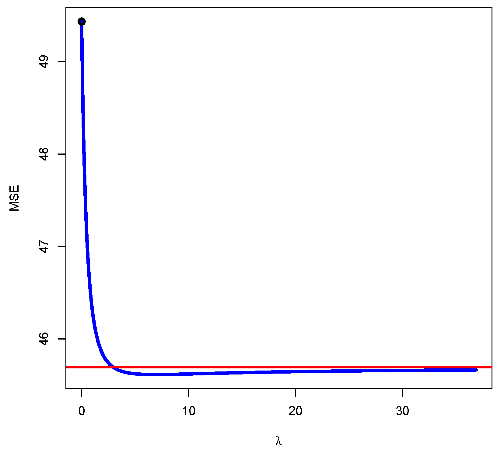
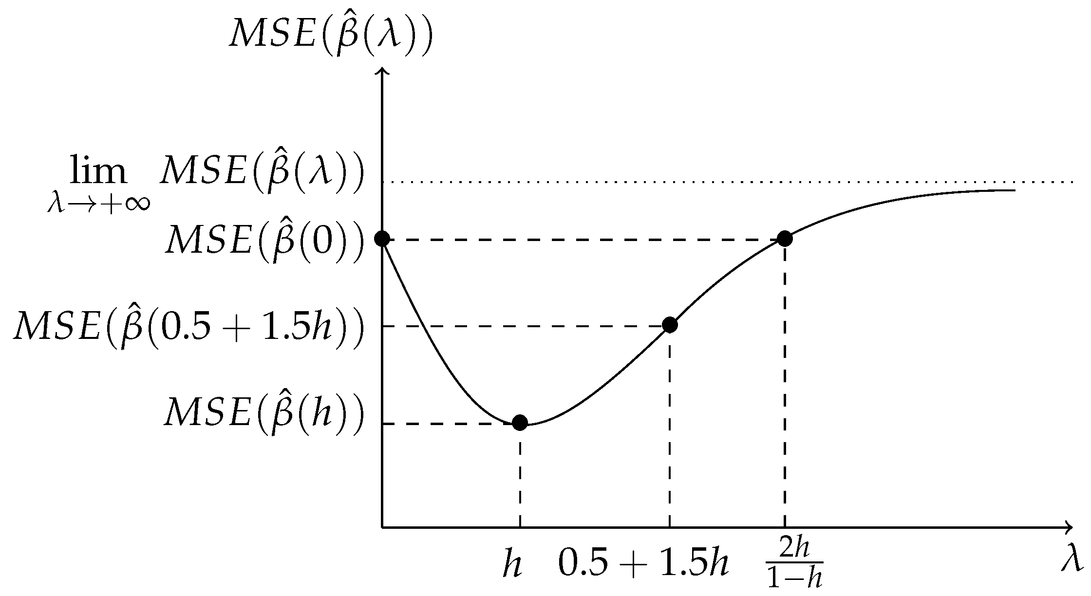
In that case, the MSE for raise regression is
MSE β ^ ( λ ) = t r V a r β ^ ( λ ) + ( E [ β ^ ( λ ) ] β ) t ( E [ β ^ ( λ ) ] β ) = σ 2 t r ( ( X ˜ t X ˜ ) 1 ) + β t ( M λ 1 I ) t ( M λ 1 I ) β = Appendix C σ 2 t r X k t X k 1 + 1 + j = 0 , j k p α ^ j 2 · β k 2 · λ 2 + h ( 1 + λ ) 2 ,
where h = σ 2 β k 2 · R S S k k .
We can obtain the MSE from the estimated values of σ 2 and β k from the model in Equation (2).
On the other hand, once the estimations are obtained and taking into account the Appendix C, λ m i n = σ ^ 2 β ^ k 2 · R S S k k minimizes MSE β ^ ( λ ) . Indeed, it is verified that MSE β ^ ( λ m i n ) < MSE β ^ ( 0 ) ; that is to say, if the goal is exclusively to minimize the MSE (as in the work presented by Hoerl et al. [33]), λ m i n should be selected as the raising factor.
Finally, note that, if λ m i n > 1 , then MSE β ^ ( λ ) < MSE β ^ ( 0 ) for all λ > 0 .

5. Numerical Examples

To illustrate the results of previous sections, two different set of data will be used that collect the two situations shown in the graphs of Figure A1 and Figure A2. The second example also compares results obtained by the raise regression to results obtained by the application of ridge and Lasso regression.

5.1. Example 1: h < 1

The data set includes different financial variables for 15 Spanish companies for the year 2016 (consolidated account and results between €800,000 and €9,000,000) obtained from the dabase Sistema de Análisis de Balances Ibéricos (SABI) database. The relationship is studied between the number of employees, E , and the fixed assets (€), FA ; operating income (€), OI ; and sales (€), S . The model is expressed as
E = β 1 + β 2 FA + β 3 OI + β 4 S + u .
Table 1 displays the results of the estimation by OLS of the model in Equation (15). The presence of essential collinearity in the model in Equation (15) is indicated by the determinant close to zero (0.0000919) of the correlation matrix of independent variables
R = 1 0.7264656 0.7225473 0.7264656 1 0.9998871 0.7225473 0.9998871 1 ,
and the VIFs (2.45664, 5200.315, and 5138.535) higher than 10. Note that the collinearity is provoked fundamentally by the relationship between OI and S.
In contrast, due to the fact that the coefficients of variation of the independent variables (1.015027, 0.7469496, and 0.7452014) are higher than 0.1002506, the threshold established as troubling by Salmerón et al. [39], it is possible to conclude that the nonessential multicollinearity is not troubling. Thus, the extension of the VIF seems appropriate to check if the application of the raise regression has mitigated the multicollinearity.
Remark 1.
λ ( 1 ) and λ ( 2 ) will be the raising factor of the first and second raising, respectively.

5.1.1. First Raising

A possible solution could be to apply the raise regression to try to mitigate the collinearity. To decide which variable is raised, the thresholds for the VIFs associated with the raise regression are calculated with the goal of raising the variable that the smaller horizontal asymptotes present. In addition to raising the variable that presents the lowest VIF, it would be interesting to obtain a lower mean squared error (MSE) after raising. For this, the λ m i n ( 1 ) is calculated for each case. Results are shown in Table 2. Note that the variable to be raised should be the second or third since their asymptotes are lower than 10, although in both cases λ m i n ( 1 ) is lower than 1 and it is not guaranteed that the MSE of the raise regression will be less than the one obtained from the estimation by the OLS of the model in Equation (15). For this reason, this table also shows the values of λ ( 1 ) that make the MSE of the raise regression coincide with the MSE of the OLS regression, λ m s e ( 1 ) , and the minimum value of λ ( 1 ) that leads to values of VIF less than 10, λ v i f ( 1 ) .
Figure 2 displays the VIF associated with the raise regression for 0 λ ( 1 ) 900 after raising the second variable. It is observed that VIFs are always higher than its corresponding horizontal asymptotes.
The model after raising the second variable will be given by
E = β 1 ( λ ) + β 2 ( λ ) FA + β 3 ( λ ) OI ˜ + β 4 ( λ ) S + u ˜ ,
where OI ˜ = OI + λ ( 1 ) · e OI with e OI the residual of regression:
OI = α 1 + α 2 FA + α 3 S + v .
Remark 2.
The coefficient of variation of OI ˜ for λ ( 1 ) = 24.5 is equal to 0.7922063; that is to say, it was lightly increased.
As can be observed from Table 3, in Equation (16), the collinearity is not mitigated by considering λ ( 1 ) equal to λ m i n ( 1 ) and λ m s e ( 1 ) . For this reason, Table 1 only shows the values of the model in Equation (16) for the value of λ ( 1 ) that leads to VIF lower than 10.

5.1.2. Transformation of Variables

After the first raising, it is interesting to verify that the VIF associated with the raise regression is invariant to data transformation. With this goal, the second variable has been raised, obtaining the V I F ( FA , λ ( 1 ) ) , V I F ( OI ˜ , λ ( 1 ) ) , and V I F ( S , λ ( 1 ) ) for λ ( 1 ) { 0 , 0.5 , 1 , 1.5 , 2 , , 95 , 10 } , supposing original, unit length, and standardized data. Next, the three possible differences and the average of the VIF associated with each variable are obtained. Table 4 displays the results from which it is possible to conclude that differences are almost null and that, consequently, the VIF associated with the raise regression is invariant to the most common data transformation.

5.1.3. Second Raising

After the first raising, we can use the results obtained from the value of λ that obtains all VIFs less than 10 or consider the results obtained for λ m i n or λ m s e and continue the procedure with a second raising. By following the second option, we part from the value of λ ( 1 ) = λ m i n ( 1 ) = 0.42 obtained after the first raising. From Table 5, the third variable is selected to be raised. Table 6 shows the VIF associated with the following model for λ m i n ( 2 ) , λ m s e ( 2 ) , and λ v i f ( 2 ) :
E = β 1 ( λ ) + β 2 ( λ ) FA + β 3 ( λ ) OI ˜ + β 4 ( λ ) S ˜ + u ˜ ,
where S ˜ = S + λ ( 2 ) · e S with e S the residuals or regression:
S = α 1 ( λ ) + α 2 ( λ ) FA + α 3 ( λ ) OI ˜ + v ˜ .
Remark 3.
The coefficient of variation of OI ˜ for λ ( 1 ) = 0.42 is equal to 0.7470222, and the coefficient of variation of S ˜ for λ ( 2 ) = 17.5 is equal to 0.7473472. In both cases, they were slightly increased.
Note than it is only possible to state that collinearity has been mitigated when λ ( 2 ) = λ v i f ( 2 ) = 17.5 . Results of this estimation are displayed in Table 1.
Considering that, after the first raising, it is obtained that λ ( 1 ) = λ m s e ( 1 ) = 1.43 , from Table 7, the third variable is selected to be raised. Table 8 shows the VIF associated with the following model for λ m i n ( 2 ) , λ m s e ( 2 ) , and λ v i f ( 2 ) :
E = β 1 ( λ ) + β 2 ( λ ) FA + β 3 ( λ ) OI ˜ + β 4 ( λ ) S ˜ + u ˜ ,
where S ˜ = S + λ · e S .
Remark 4.
The coefficient of variation of OI ˜ for λ ( 1 ) = 1.43 is equal to 0.7473033, and the coefficient of variation of S ˜ for λ ( 2 ) = 10 is equal to 0.7651473. In both cases, they were lightly increased.
Remark 5.
Observing the coefficients of variation of OI ˜ for different raising factor. it is concluded that the coefficient of variation increases as the raising factor increases: 0.7470222 ( λ = 0.42 ), 0.7473033 ( λ = 1.43 ), and 0.7922063 ( λ = 24.5 ).
Note that it is only possible to state that collinearity has been mitigated when λ ( 2 ) = λ v i f ( 2 ) = 10 . Results of the estimations of this model are shown in Table 1.

5.1.4. Interpretation of Results

Analyzing the results of Table 1, it is possible to conclude that
  • In the model in Equation (16) (in which the second variable is raised considering the smallest λ that makes all the VIFs less than 10, λ ( 1 ) = 24.5 ), the variable sales have a coefficient significantly different from zero, where in the original model this was not the case. In this case, the MSE is superior to the one obtained by OLS.
  • In the model in Equation (17) (in which the second variable is raised considering the value of λ that minimizes the MSE, λ ( 1 ) = 0.42 , and after that, the third variable is raised considering the smallest λ that makes all the VIFs less than 10, λ ( 2 ) = 17.5 ), there is no difference in the individual significance of the coefficient.
  • In the model in Equation (18) (in which the second variable is raised considering the value of λ that makes the MSE of the raise regression coincide with that of OLS, λ ( 1 ) = 1.43 , and next, the third variable is raised considering the smallest λ that makes all the VIFs less than 10, λ ( 2 ) = 10 ), there is no difference in the individual significance of the coefficient.
  • Although the coefficient of variable OI is not significantly different from zero in any case, the not expected negative sign obtained in model in Equation (15) is corrected in models Equations (17) and (18).
  • In the models with one or two raisings, all the global characteristics coincide with that of the model in Equation (15). Furthermore, there is a relevant decrease in the estimation of the standard deviation for the second and third variable.
  • In models with one or two raisings, the MSE increases, with the model in Equation (16) being the one that presents the smallest MSE among the biased models.
Thus, in conclusion, the model in Equation (16) is selected as it presents the smallest MSE and there is an improvement in the individual significance of the variables.

5.2. Example 2: h > 1

This example uses the following model previously applied by Klein and Goldberger [43] about consumption and salaries in the United States from 1936 to 1952 (1942 to 1944 were war years, and data are not available):
C = β 1 + β 2 WI + β 3 NWI + β 4 FI + u ,
where C is consumption, WI is wage income, NWI is non-wage, non-farm income, and FI is the farm income. Its estimation by OLS is shown in Table 9.
However, this estimation is questionable since no estimated coefficient is significantly different to zero while the model is globally significant (with 5% significance level), and the VIFs associated with each variable (12.296, 9.23, and 2.97) indicate the presence of severe essential collinearity. In addition, the determinant of the matrix of correlation
R = 1 0.9431118 0.8106989 0.9431118 1 0.7371272 0.8106989 0.7371272 1 ,
is equal to 0.03713592 and, consequently, lower than the threshold recommended by García et al. [44] ( 1.013 · 0.1 + 0.00008626 · n 0.01384 · p = 0.04714764 being n = 14 and p = 4 ); it is maintained the conclusion that the near multicollinearity existing in this model is troubling.
Once again, the values of the coefficients of variation (0.2761369, 0.2597991, and 0.2976122) indicate that the nonessential multicollinearity is not troubling (see Salmerón et al. [39]). Thus, the extension of the VIF seems appropriate to check if the application of the raise regression has mitigated the near multicollinearity.
Next, it is presented the estimation of the model by raise regression and the results are compared to the estimation by ridge and Lasso regression.

5.2.1. Raise Regression

When calculating the thresholds that would be obtained for VIFs by raising each variable (see Table 10), it is observed that, in all cases, they are less than 10. However, when calculating λ m i n in each case, a value higher than one is only obtained when raising the third variable. Figure 3 displays the MSE for λ [ 0 , 37 ) . Note that M S E ( β ^ ( λ ) ) is always less than the one obtained by OLS, 49.434, and presents an asymptote in lim λ + M S E ( β ^ ( λ ) ) = 45.69422 .
The following model is obtained by raising the third variable:
C = β 1 ( λ ) + β 2 ( λ ) WI + β 3 ( λ ) NWI + β 4 ( λ ) FI ˜ + u ˜ ,
where FI ˜ = FI + λ · e FI being e FI the residuals of regression:
FI = α 1 + α 2 WI + α 3 NWI + v .
Remark 6.
The coefficient of variation FI ˜ for λ ( 1 ) = 6.895 is 1.383309. Thus, the application of the raise regression has mitigated the nonessential multicollinearity in this variable.
Table 9 shows the results for the model in Equation (20), being λ = 6.895 . In this case, the MSE is the lowest possible for every possible value of λ and lower than the one obtained by OLS for the model in Equation (19). Furthermore, in this case, the collinearity is not strong once all the VIF are lower than 10 (9.098, 9.049, and 1.031, respectively). However, the individual significance in the variable was not improved.
With the purpose of improving this situation, another variable is raised. If the first variable is selected to be raised, the following model is obtained:
C = β 1 ( λ ) + β 2 ( λ ) WI ˜ + β 3 ( λ ) NWI + β 4 ( λ ) FI + u ˜ ,
where WI ˜ = WI + λ · e WI being e WI the residuals of regression:
WI = α 1 + α 2 NWI + α 3 FI + v .
Remark 7.
The coefficient of variation of WI ˜ for λ ( 1 ) = 0.673 is 0.2956465. Thus, it is noted that the raise regression has lightly mitigated the nonessential mutlicollinearity of this variable.
Table 9 shows the results for the model in Equation (21), being λ = 0.673 . In this case, the MSE is lower than the one obtained by OLS for the model in Equation (19). Furthermore, in this case, the collinearity is not strong once all the VIF are lower than 10 (5.036024, 4.705204, and 2.470980, respectively). Note that raising this variable, the values of VIFs are lower than raising the first variable but the MSE is higher. However, this model is selected as preferable due to the individual significance being better in this model and the MSE being lower than the one obtained by OLS.

5.2.2. Ridge Regression

This subsection presents the estimation of the model in Equation (19) by ridge regression (see Hoerl and Kennard [4] or Marquardt [45]). The first step is the selection of the appropriate value of K.
The following suggestions are addressed:
  • Hoerl et al. [33] proposed the value of K H K B = p · σ ^ 2 β ^ t β ^ since probability higher than 50% leads to a MSE lower than the one from OLS.
  • García et al. [26] proposed the value of K, denoted as K V I F , that leads to values of VIF lower than 10 (threshold traditionally established as troubling).
  • García et al. [44] proposed the following values:
    K e x p = 0.006639 · e 1 d e t ( R ) 0.00001241 · n + 0.005745 · p , K l i n e a r = 0.01837 · ( 1 d e t ( R ) ) 0.00001262 · n + 0.005678 · p , K s q = 0.7922 · ( 1 d e t ( R ) ) 2 0.6901 · ( 1 d e t ( R ) ) 0.000007567 · n 0.01081 · p ,
    where d e t ( R ) denotes the determinant of the matrix of correlation, R .
The following values are obtained K H K B = 0.417083 , K V I F = 0.013 , K e x p = 0.04020704 , K l i n e a r = 0.04022313 , and K s q = 0.02663591 .
Table 11 and Table 12 show (The results for K l i n e a r are not considered as they are very similar to results obtained by K e x p .) the estimations obtained from ridge estimators (expression (1)) and the individual significance intervals obtained by bootstrap considering percentiles 5 and 95 for 5000 repeats. It is also calculated the goodness of the fit by following the results shown by Rodríguez et al. [28] and the MSE.
Note that only the constant term can be considered significatively different to zero and that, curiously, the value of K proposed by Hoerl et al. [33] leads to a value of MSE higher than the one from OLS while the values proposed by García et al. [26] and García et al. [44] lead to a value of MSE lower than the one obtained by OLS. All cases lead to values of VIF lower than 10; see García et al. [26] for its calculation:
2.0529 , 1.8933 and 1.5678 for K H K B , 9.8856 , 7.5541 and 2.7991 for K V I F , 7.1255 , 5.6191 and 2.5473 for K e x p , 8.2528 , 6.4123 and 2.65903 for K s q .
In any case, the lack of individual significance justifies the selection of the raise regression as preferable in comparison to the models obtained by ridge regression.

5.2.3. Lasso Regression

The Lasso regression (see Tibshirani [5]) is a method initially designed to select variables constraining the coefficient to zero, being specially useful in models with a high number of independent variables. However, this estimation methodology has been widely applied in situation where the model presents worrying near multicollinearity.
Table 13 shows results obtained by the application of the Lasso regression to the model in Equation (19) by using the package glmnet of the programming environment R Core Team [46]. Note that these estimations are obtained for the optimal value of λ = 0.1258925 obtained after a k-fold cross-validation.
The inference obtained by bootstrap methodology (with 5000 repeats) allows us to conclude that in, at least, the 5% of the cases, the coefficient of NWI is constrained to zero. Thus, this variable should be eliminated from the model.
However, we consider that this situation should be avoided, and as an alternative to the elimination of variable, that is, as an alternative from the following model, the estimation by raise or ridge regression is proposed.
C = π 1 + π 2 WI + π 3 FI + ϵ ,
It could be also appropriate to apply the residualization method (see, for example, York [47], Salmerón et al. [48], and García et al. [44]), which consists in the estimation of the following model:
C = τ 1 + τ 2 WI + τ 3 FI + τ 4 res NWI + ε ,
where, for example, res NWI represents the residuals of the regression of NWI as a function of WI that will be interpreted as the part of NWI not related to WI . In this case (see García et al. [44]), it is verified that π ^ i = τ ^ i for i = 1 , 2 , 3 . That is to say, the model in Equation (23) estimates the same relationship between WI and FI with C as in the model in Equation (22) with the benefit that the variable NWI is not eliminated due to a part of it being considered.

6. Conclusions

The Variance Inflation Factor (VIF) is one of the most applied measures to diagnose collinearity together with the Condition Number (CN). Once the collinearity is detected, different methodologies can be applied as, for example, the raise regression, but it will be required to check if the methodology has mitigated the collinearity effectively. This paper extends the concept of VIF to be applied after the raise regression and presents an expression of the VIF that verifies the following desirable properties (see García et al. [26]):
  • continuous in zero. That is to say, when the raising factor ( λ ) is zero, the VIF obtained in the raise regression coincides with the one obtained by OLS;
  • decreasing as a function of the raising factor ( λ ). That is to say, the degree of collinearity diminishes as λ increases, and
  • always equal or higher than 1.
The paper also shows that the VIF in the raise regression is scale invariant, which is a very common transformation when working with models with collinearity. Thus, it yields identical results regardless of whether predictions are based on unstandardized or standardized predictors. Contrarily, the VIFs obtained from other penalized regressions (ridge regression, Lasso, and Elastic Net) are not scale invariant and hence yield different results depending on the predictor scaling used.
Another contribution of this paper is the analysis of the asymptotic behavior of the VIF associated with the raised variable (verifying that its limit is equal to 1) and associated with the rest of the variables (presenting an horizontal asymptote). This analysis allows to conclude that
  • It is possible to know a priori how far each of the VIFs can decrease simply by calculating their horizontal asymptote. This could be used as a criterion to select the variable to be raised, the one with the lowest horizontal asymptote being chosen.
  • If there is asymptote under the threshold established as worrying, the extension of the VIF can be applied to select the raising factor considering the value of λ that verifies V I F ( k , λ ) < 10 for k = 2 , , p .
  • It is possible that the collinearity is not mitigated with any value of λ . This can happen when at least one horizontal asymptote is greater than the threshold. In that case, a second variable has to be raised. García and Ramírez [42] and García et al. [31] show the successive raising procedure.
On the other hand, since the raise estimator is biased, the paper analyzes its Mean Square Error (MSE), showing that there is a value of λ that minimizes the possibility of the MSE being lower than the one obtained by OLS. However, it is not guaranteed that the VIF for this value of λ presents a value less than the established thresholds. The results are illustrated with two numerical examples, and in the second one, the results obtained by OLS are compared to the results obtained with the raise, ridge, and Lasso regressions that are widely applied to estimated models with worrying multicollinearity. It is showed that the raise regression can compete and even overcome these methodologies.
Finally, we propose as future lines of research the following questions:
  • The examples showed that the coefficients of variation increase after raising the variables. This fact is associated with an increase in the variability of the variable and, consequently, with a decrease of the near nonessential multicollinearity. Although a deeper analysis is required, it seems that raise regression mitigates this kind of near multicollinearity.
  • The value of the ridge factor traditionally applied, K H K B , leads to estimators with smaller MSEs than the OLS estimators with probability greater than 0.5. In contrast, the value of the raising factor λ m i n always leads to estimators with smaller MSEs than OLS estimators. Thus, it is deduced that the ridge regression provides estimators with MSEs higher than the MSEs of OLS estimators with probability lower than 0.5. These questions seem to indicate that, in terms of MSE, the raise regression can present better behaviour than the ridge regression. However, the confirmation of this judgment will require a more complete analysis, including other aspects such as interpretability and inference.

Author Contributions

Conceptualization, J.G.P., C.G.G. and R.S.G. and A.R.S.; methodology, R.S.G. and A.R.S.; software, A.R.S.; validation, J.G.P., R.S.G. and C.G.G.; formal analysis, R.S.G. and C.G.G.; investigation, R.S.G. and A.R.S.; writing—original draft preparation, A.R.S. and C.G.G.; writing—review and editing, C.G.G.; supervision, J.G.P. All authors have read and agreed to the published version of the manuscript.

Funding

This research received no external funding.

Acknowledgments

We thank the anonymous referees for their useful suggestions.

Conflicts of Interest

The authors declare no conflict of interest.

Appendix A

Given the linear model in Equation (7), it is obtained that
α ^ ( λ ) = X i , j t X i , j X i , j t X ˜ i X ˜ i t X i , j X ˜ i t X ˜ i 1 · X i , j t X j X ˜ i t X j = X i , j t X i , j X i , j t X i X i t X i , j X i t X i + ( λ 2 + 2 λ ) R S S i i 1 · X i , j t X j X i t X j = A ( λ ) B ( λ ) B ( λ ) t C ( λ ) · X i , j t X j X i t X j = A ( λ ) · X i , j t X j + B ( λ ) · X i t X j B ( λ ) t · X i , j t X j + C ( λ ) · X i t X j = α ^ i , j ( λ ) α ^ i ( λ ) ,
Since it is verified that e i t X i , j = 0 , then X ˜ i t X i , j = ( X i + λ e i ) t X i , j = X i t X i , j , where
C ( λ ) = X i t X i + ( λ 2 + 2 λ ) R S S i i X i t X i , j X i , j t X i , j 1 X i , j t X i 1 = X i t I X i , j X i , j t X i , j 1 X i , j t X i + ( λ 2 + 2 λ ) R S S i i 1 = R S S i i , j + ( λ 2 + 2 λ ) R S S i i 1 , B ( λ ) = X i , j t X i , j 1 X i , j t X i · C ( λ ) = R S S i i , j R S S i i , j + ( λ 2 + 2 λ ) R S S i i · B , A ( λ ) = X i , j t X i , j 1 + X i , j t X i , j 1 X i , j t X i · C ( λ ) · X i t X i , j X i , j t X i , j 1 = X i , j t X i , j 1 + ( R S S i i , j ) 2 R S S i i , j + ( λ 2 + 2 λ ) R S S i i · B · B t .
Then,
α ^ i , j ( λ ) = X i , j t X i , j 1 X i , j t X j + ( R S S i i , j ) 2 R S S i i , j + ( λ 2 + 2 λ ) R S S i i · B · B t · X i , j t X j + R S S i i , j R S S i i , j + ( λ 2 + 2 λ ) R S S i i · B · X i t X j = X i , j t X i , j 1 X i , j t X j + R S S i i , j R S S i i , j · B · B t · X i , j t X j + B · X i t X j R S S i i , j + ( λ 2 + 2 λ ) R S S i i , α ^ i ( λ ) = R S S i i , j R S S i i , j + ( λ 2 + 2 λ ) R S S i i · B t · X i , j t X j + 1 R S S i i , j + ( λ 2 + 2 λ ) R S S i i · X i t X j = R S S i i , j R S S i i , j + ( λ 2 + 2 λ ) R S S i i · B t · X i , j t X j + ( R S S i i , j ) 1 X i t X j = R S S i i , j R S S i i , j + ( λ 2 + 2 λ ) R S S i i · α ^ i .

Appendix B

Given the linear model
X j = X j α + v = X i , j X i α i , j α i + v ,
it is obtained that
α ^ = X i , j t X i , j X i , j t X i X i t X i , j X i t X i 1 · X i , j t X j X i t X j = A B B t C · X i , j t X j X i t X j = A · X i , j t X j + B · X i t X j B t · X i , j t X j + C · X i t X j = α ^ i , j α ^ i ,
where
C = X i t X i X i t X i , j X i , j t X i , j 1 X i , j t X i 1 = X i t I X i , j X i , j t X i , j 1 X i , j t X i 1 = R S S i i , j 1 , B = X i , j t X i , j 1 X i , j t X i · C , A = X i , j t X i , j 1 · I + X i , j t X i · C · X i t X i , j X i , j t X i , j 1 = X i , j t X i , j 1 + 1 C · B · B t .
In that case, the residual sum of squares is given by
R S S j j = X j t X j A · X i , j t X j + B · X i t X j B t · X i , j t X j + C · X i t X j t X i , j t X j X i t X j = X j t X j X j t X i , j · A t · X i , j t X j X j t X i · B t · X i , j t X j α ^ i t X i t X j = X j t X j X j t X i , j X i , j t X i , j 1 X i , j t X j R S S i i , j X j t X i , j · B · B t · X i , j t X j X j t X i · B t · X i , j t X j α ^ i t X i t X j = R S S j i , j R S S i i , j X j t X i , j · B · B t · X i , j t X j + X j t X i · B t · X i , j t X j + α ^ i t X i t X j ,
and consequently
R S S j i , j R S S j j = R S S i i , j X j t X i , j · B · B t · X i , j t X j + X j t X i · B t · X i , j t X j + α ^ i t X i t X j .

Appendix C

First, parting from the expression Equation (14), it is obtained that
M λ 1 = 1 0 0 λ 1 + λ α ^ 0 0 0 0 1 0 λ 1 + λ α ^ 1 0 0 0 0 1 ( 1 ) k 1 λ 1 + λ α ^ k 1 0 0 0 0 0 1 1 + λ 0 0 0 0 0 ( 1 ) k + 1 λ 1 + λ α ^ k + 1 1 0 0 0 0 ( 1 ) p λ 1 + λ α ^ p 0 1 ,
and then,
( M λ 1 I ) t ( M λ 1 I ) = 0 0 0 0 0 0 0 0 0 0 0 0 0 0 0 0 0 0 0 0 0 a ( λ ) 0 0 0 0 0 0 0 0 0 0 0 0 0 0 ,
where a ( λ ) = λ 2 ( 1 + λ ) 2 · α ^ 0 + α ^ 1 + + α ^ k 1 2 + 1 + α ^ k + 1 2 + + α ^ p 2 . In that case,
β t ( M λ 1 I ) t ( M λ 1 I ) β = a ( λ ) · β k 2 .
Second, partitioning X ˜ in the form X ˜ = X k X ˜ k , it is obtained that
X ˜ t X ˜ 1 = X k t X k 1 + α ^ α ^ t ( 1 + λ ) 2 · e k t e k α ^ ( 1 + λ ) 2 · e k t e k α ^ t ( 1 + λ ) 2 · e k t e k 1 ( 1 + λ ) 2 · e k t e k ,
and then,
t r ( ( X ˜ t X ˜ ) 1 ) = t r X k t X k 1 + 1 ( 1 + λ ) 2 · e k t e k · t r α ^ α ^ t + 1 .
Consequently, it is obtained that
MSE β ^ ( λ ) = σ 2 t r X k t X k 1 + 1 + j = 0 , j k p α ^ j 2 · β k 2 · λ 2 + h ( 1 + λ ) 2 ,
where h = σ 2 β k 2 · R S S k k .
Third, taking into account that the first and second derivatives of expression Equation (A1) are, respectively,
λ MSE β ^ ( λ ) = 1 + j = 0 , j k p α ^ j 2 · β k 2 · 2 ( λ h ) ( 1 + λ ) 3 , 2 λ 2 MSE β ^ ( λ ) = 2 1 + j = 0 , j k p α ^ j 2 · β k 2 · 2 λ ( 1 + 3 h ) ( 1 + λ ) 4 .
Since λ 0 , it is obtained that MSE β ^ ( λ ) is decreasing if λ < h and increasing if λ > h , and it is concave if λ > 1 + 3 h 2 and convex if λ < 1 + 3 h 2 .
Indeed, given that
lim λ + MSE β ^ ( λ ) = σ 2 t r X k t X k 1 + 1 + j = 0 , j k p α ^ j 2 · β k 2 , MSE β ^ ( 0 ) = σ 2 t r X k t X k 1 + 1 + j = 0 , j k p α ^ j 2 · β k 2 · h ,
if h > 1 , then MSE β ^ ( 0 ) > lim λ + MSE β ^ ( λ ) , and if h < 1 , then MSE β ^ ( 0 ) < lim λ + MSE β ^ ( λ ) . That is to say, if h > 1 , then the raise estimator presents always a lower MSE than the one obtained by OLS for all λ , and comparing expressions Equations (A1) and (A2) when h < 1 , MSE β ^ ( λ ) MSE β ^ ( 0 ) if λ 2 · h 1 h .
From this information, the behavior of the MSE is represented in Figure A1 and Figure A2. Note that the MSE presents a minimum value for λ = h .
Figure A1. M S E ( β ^ ( λ ) ) representation for h = σ 2 ( e k t e k ) · β k 2 < 1 .
Mathematics 08 00605 g0a1
Figure A2. M S E ( β ^ ( λ ) ) representation for h = σ 2 ( e k t e k ) · β k 2 > 1 .
Mathematics 08 00605 g0a2

References

  1. Kiers, H.; Smilde, A. A comparison of various methods for multivariate regression with highly collinear variables. Stat. Methods Appl. 2007, 16, 193–228. [Google Scholar] [CrossRef]
  2. Frank, L.E.; Friedman, J.H. A statistical view of some chemometrics regression tools. Technometrics 1993, 35, 109–135. [Google Scholar] [CrossRef]
  3. Fu, W.J. Penalized regressions: the bridge versus the lasso. J. Comput. Graph. Stat. 1998, 7, 397–416. [Google Scholar]
  4. Hoerl, A.E.; Kennard, R.W. Ridge regression: Biased estimation for nonorthogonal problems. Technometrics 1970, 12, 55–67. [Google Scholar] [CrossRef]
  5. Tibshirani, R. Regression shrinkage and selection via the lasso. J. R. Stat. Soc. Ser. B (Methodol.) 1996, 58, 267–288. [Google Scholar] [CrossRef]
  6. Donoho, D.L.; Johnstone, I.M. Adapting to unknown smoothness via wavelet shrinkage. J. Am. Stat. Assoc. 1995, 90, 1200–1224. [Google Scholar] [CrossRef]
  7. Klinger, A. Inference in high dimensional generalized linear models based on soft thresholding. J. R. Stat. Soc. Ser. B (Stat. Methodol.) 2001, 63, 377–392. [Google Scholar] [CrossRef] [Green Version]
  8. Dupuis, D.; Victoria-Feser, M. Robust VIF regression with application to variable selection in large data sets. Ann. Appl. Stat. 2013, 7, 319–341. [Google Scholar] [CrossRef]
  9. Li, Y.; Yang, H. A new Liu-type estimator in linear regression model. Stat. Pap. 2012, 53, 427–437. [Google Scholar] [CrossRef]
  10. Liu, Y.; Wang, Y.; Feng, Y.; Wall, M. Variable selection and prediction with incomplete high-dimensional data. Ann. Appl. Stat. 2016, 10, 418–450. [Google Scholar] [CrossRef]
  11. Uematsu, Y.; Tanaka, S. High-dimensional macroeconomic forecasting and variable selection via penalized regression. Econom. J. 2019, 22, 34–56. [Google Scholar] [CrossRef]
  12. Zou, H.; Hastie, T. Regularization and variable selection via the elastic net. J. R. Stat. Soc. Ser. B (Stat. Methodol.) 2005, 67, 301–320. [Google Scholar] [CrossRef] [Green Version]
  13. Tutz, G.; Ulbricht, J. Penalized regression with correlation-based penalty. Stat. Comput. 2009, 19, 239–253. [Google Scholar] [CrossRef] [Green Version]
  14. Stone, M.; Brooks, R.J. Continuum regression: Cross-validated sequentially constructed prediction embracing ordinary least squares, partial least squares and principal components regression. J. R. Stat. Soc. Ser. B (Methodol.) 1990, 52, 237–269. [Google Scholar] [CrossRef]
  15. Efron, B.; Hastie, T.; Johnstone, I.; Tibshirani, R. Least angle regression. Ann. Stat. 2004, 32, 407–499. [Google Scholar]
  16. Golan, A.; Judge, G.; Miller, D. Maximum Entropy Econometrics: Robust Estimation With Limited Data; John Wiley and Sons: Chichester, UK, 1997. [Google Scholar]
  17. Golan, A. Information and entropy econometrics review and synthesis. Found. Trends Econom. 2008, 2, 1–145. [Google Scholar] [CrossRef]
  18. Macedo, P. Ridge Regression and Generalized Maximum Entropy: An improved version of the Ridge–GME parameter estimator. Commun. Stat.-Simul. Comput. 2017, 46, 3527–3539. [Google Scholar] [CrossRef]
  19. Batah, F.S.M.; Özkale, M.R.; Gore, S. Combining unbiased ridge and principal component regression estimators. Commun. Stat. Theory Methods 2009, 38, 2201–2209. [Google Scholar] [CrossRef]
  20. Massy, W.F. Principal components regression in exploratory statistical research. J. Am. Stat. Assoc. 1965, 60, 234–256. [Google Scholar] [CrossRef]
  21. Guo, W.; Liu, X.; Zhang, S. The principal correlation components estimator and its optimality. Stat. Pap. 2016, 57, 755–779. [Google Scholar] [CrossRef]
  22. Aguilera-Morillo, M.; Aguilera, A.; Escabias, M.; Valderrama, M. Penalized spline approaches for functional logit regression. Test 2013, 22, 251–277. [Google Scholar] [CrossRef]
  23. Wold, S.; Sjöström, M.; Eriksson, L. PLS-regression: A basic tool of chemometrics. Chemom. Intell. Lab. Syst. 2001, 58, 109–130. [Google Scholar] [CrossRef]
  24. De Jong, S. SIMPLS: An alternative approach to partial least squares regression. Chemom. Intell. Lab. Syst. 1993, 18, 251–263. [Google Scholar] [CrossRef]
  25. Jensen, D.; Ramirez, D. Surrogate models in ill-conditioned systems. J. Stat. Plan. Inference 2010, 140, 2069–2077. [Google Scholar] [CrossRef]
  26. García, J.; Salmerón, R.; García, C.; López Martín, M.D.M. Standardization of variables and collinearity diagnostic in ridge regression. Int. Stat. Rev. 2016, 84, 245–266. [Google Scholar] [CrossRef]
  27. Marquardt, D. You should standardize the predictor variables in your regression models. Discussion of: A critique of some ridge regression methods. J. Am. Stat. Assoc. 1980, 75, 87–91. [Google Scholar]
  28. Rodríguez, A.; Salmerón, R.; García, C. The coefficient of determination in the ridge regression. Commun. Stat. Simul. Comput. 2019. [Google Scholar] [CrossRef] [Green Version]
  29. García, C.G.; Pérez, J.G.; Liria, J.S. The raise method. An alternative procedure to estimate the parameters in presence of collinearity. Qual. Quant. 2011, 45, 403–423. [Google Scholar] [CrossRef]
  30. Salmerón, R.; García, C.; García, J.; López, M.D.M. The raise estimator estimation, inference, and properties. Commun. Stat. Theory Methods 2017, 46, 6446–6462. [Google Scholar] [CrossRef]
  31. García, J.; López-Martín, M.; García, C.; Salmerón, R. A geometrical interpretation of collinearity: A natural way to justify ridge regression and its anomalies. Int. Stat. Rev. 2020. [Google Scholar] [CrossRef]
  32. Belsley, D.A.; Kuh, E.; Welsch, R.E. Regression Diagnostics: Identifying Influential Data and Sources of Collinearity; John Wiley & Sons: Hoboken, NJ, USA, 2005; Volume 571. [Google Scholar]
  33. Hoerl, A.; Kannard, R.; Baldwin, K. Ridge regression: some simulations. Commun. Stat. Theory Methods 1975, 4, 105–123. [Google Scholar] [CrossRef]
  34. Stein, C. Inadmissibility of the Usual Estimator for the Mean of a Multivariate Normal Distribution. In Proceedings of the Third Berkeley Symposium on Mathematical Statistics and Probability, Volume 1: Contributions to the Theory of Statistics; University of California Press: Berkeley, CA, USA, 1956; pp. 197–206. [Google Scholar]
  35. James, W.; Stein, C. Estimation with Quadratic Loss. In Proceedings of the Fourth Berkeley Symposium on Mathematical Statistics and Probability, Volume 1: Contributions to the Theory of Statistics; University of California Press: Berkeley, CA, USA, 1961; pp. 361–379. [Google Scholar]
  36. Ohtani, K. An MSE comparison of the restricted Stein-rule and minimum mean squared error estimators in regression. Test 1998, 7, 361–376. [Google Scholar] [CrossRef]
  37. Hubert, M.; Gijbels, I.; Vanpaemel, D. Reducing the mean squared error of quantile-based estimators by smoothing. Test 2013, 22, 448–465. [Google Scholar] [CrossRef]
  38. Salmerón, R.; García, C.; García, J. Variance Inflation Factor and Condition Number in multiple linear regression. J. Stat. Comput. Simul. 2018, 88, 2365–2384. [Google Scholar] [CrossRef]
  39. Salmerón, R.; Rodríguez, A.; García, C. Diagnosis and quantification of the non-essential collinearity. Comput. Stat. 2019. [Google Scholar] [CrossRef]
  40. Marquandt, D.; Snee, R. Ridge regression in practice. Am. Stat. 1975, 29, 3–20. [Google Scholar]
  41. García, C.B.; Garcí, J.; Salmerón, R.; López, M.M. Raise regression: Selection of the raise parameter. In Proceedings of the International Conference on Data Mining, Vancouver, BC, Canada, 30 April–2 May 2015. [Google Scholar]
  42. García, J.; Ramírez, D. The successive raising estimator and its relation with the ridge estimator. Commun. Stat. Simul. Comput. 2016, 46, 11123–11142. [Google Scholar] [CrossRef]
  43. Klein, L.; Goldberger, A. An Economic Model of the United States, 1929–1952; North Holland Publishing Company: Amsterdan, The Netherlands, 1964. [Google Scholar]
  44. García, C.; Salmerón, R.; García, C.; García, J. Residualization: Justification, properties and application. J. Appl. Stat. 2019. [Google Scholar] [CrossRef]
  45. Marquardt, D. Generalized inverses, ridge regression, biased linear estimation, and nonlinear estimation. Technometrics 1970, 12, 591–612. [Google Scholar] [CrossRef]
  46. R Core Team. R: A Language and Environment for Statistical Computing; R Foundation for Statistical Computing: Vienna, Austria, 2017. [Google Scholar]
  47. York, R. Residualization is not the answer: Rethinking how to address multicollinearity. Soc. Sci. Res. 2012, 41, 1379–1386. [Google Scholar] [CrossRef]
  48. Salmerón, R.; García, J.; García, C.; García, C. Treatment of collinearity through orthogonal regression: An economic application. Boletín Estadística Investig. Oper. 2016, 32, 184–202. [Google Scholar]
Figure 1. Representation of the raise method.
Mathematics 08 00605 g001
Figure 2. VIF of the variables after raising OI .
Mathematics 08 00605 g002
Figure 3. Mean square error (MSE) for the model in Equation (19) after raising third variable.
Mathematics 08 00605 g003
Table 1. Estimations of the models in Equations (15)–(18): Standard deviation is inside the parenthesis, R 2 is the coefficient of determination, F 3 , 11 is the experimental value of the joint significance contrast, and σ ^ 2 is the variance estimate of the random perturbation.
Model (15)p-ValueModel (16) for λ vif ( 1 ) = 24.5 p-ValueModel (17) for λ min ( 1 ) = 0.42 and λ vif ( 2 ) = 17.5 p-ValueModel (18) for λ mse ( 1 ) = 1.43 and λ vif ( 2 ) = 10 p-Value
Intercept994.21 (17,940)0.9574588.68 (17,773.22)0.8015257.84 (1744.26)0.7725582.29 (17,740.18)0.759
FA −1.28 (0.55)0.039−1.59 (0.50)0.009−1.59 (0.51)0.009−1.58 (0.51)0.009
OI −81.79 (52.86)0.150
OI ˜ λ v i f ( 1 ) −3.21 (2.07)0.150
OI ˜ λ m i n ( 1 ) 1.67 (2.28)0.478
OI ˜ λ m s e ( 1 ) 1.51 (2.24)0.517
S 87.58 (53.29)0.1298.38 (2.35)0.004
S ˜ λ v i f ( 2 ) 3.42 (2.03)0.1203.55 (1.99)0.103
R 2 0.70 0.70 0.70 0.70
F 3 , 11 8.50 8.50 8.50 8.50
σ ^ 2 1,617,171,931 1,617,171,931 1,617,171,931 1,617,171,931
MSE321,730,738 321,790,581 336,915,567 325,478,516
Table 2. Horizontal asymptotes for variance inflation factors (VIF) after raising each variable and λ m i n ( 1 ) , λ m s e ( 1 ) , and λ v i f ( 1 ) .
Raised lim λ ( 1 ) + VIF ( FA , λ ( 1 ) ) lim λ ( 1 ) + VIF ( OI , λ ( 1 ) ) lim λ ( 1 ) + VIF ( S , λ ( 1 ) )
Variable 114429.224429.22
Variable 22.0912.09
Variable 32.122.121
Raised λ m i n ( 1 ) λ m s e ( 1 ) λ v i f ( 1 )
Variable 10.180.45
Variable 20.421.4324.5
Variable 30.371.1824.7
Table 3. VIF of regression Equation (16) for λ ( 1 ) equal to λ m i n ( 1 ) , λ m s e ( 1 ) , and λ v i f ( 1 ) .
VIF ( FA , λ ( 1 ) ) VIF ( OI ˜ , λ ( 1 ) ) VIF ( S , λ ( 1 ) )
λ m i n ( 1 ) 2.272587.842557.66
λ m s e ( 1 ) 2.15878.10868.58
λ v i f ( 1 ) 2.099.009.99
Table 4. Effect of data transformations on VIF associated with raise regression.
VIF ( FA , λ ( 1 ) ) VIF ( OE ˜ , λ ( 1 ) ) VIF ( S , λ ( 1 ) )
Original–Unit length 9.83 · 10 16 1.55 · 10 11 1.83 · 10 10
Original–Standardized 1.80 · 10 16 3.10 · 10 10 2.98 · 10 10
Unit length–Standardized 1.16 · 10 15 3.26 · 10 10 1.15 · 10 10
Table 5. Horizontal asymptote for VIFs after raising each variable in the second raising for λ m i n ( 2 ) , λ m s e ( 2 ) and λ v i f ( 2 ) .
Raised lim λ ( 2 ) + VIF ( FA , λ ( 2 ) ) lim λ ( 2 ) + VIF ( OI ˜ , λ ( 2 ) ) lim λ ( 2 ) + VIF ( S , λ ( 2 ) )
Variable 112381.562381.56
Variable 32.122.121
Raised λ m i n ( 2 ) λ m s e ( 2 ) λ v i f ( 2 )
Variable 10.150.34
Variable 30.351.0917.5
Table 6. VIFs of regression Equation (16) for λ ( 2 ) equal to λ m i n ( 2 ) , λ m s e ( 2 ) , and λ v i f ( 2 ) .
VIF ( FA , λ ( 2 ) ) VIF ( OI ˜ , λ ( 2 ) ) VIF ( S ˜ , λ ( 2 ) )
λ m i n ( 2 ) 2.201415.061398.05
λ m s e ( 2 ) 2.15593.98586.20
λ v i f ( 2 ) 2.129.678.47
Table 7. Horizontal asymptote for VIFs after raising each variables in the second raising for λ m i n ( 2 ) , λ m s e ( 2 ) , and λ v i f ( 2 ) .
Raised lim λ ( 2 ) + VIF ( FA , λ ( 2 ) ) lim λ ( 2 ) + VIF ( OI ˜ , λ ( 2 ) ) lim λ ( 2 ) + VIF ( S , λ ( 2 ) )
Variable 11853.40853.40
Variable 32.122.121
Raised λ m i n ( 2 ) λ m s e ( 2 ) λ v i f ( 2 )
Variable 10.120.27
Variable 30.320.9210
Table 8. VIFs of regression Equation (16) for λ ( 2 ) equal to λ m i n ( 2 ) , λ m s e ( 2 ) , and λ v i f ( 2 ) .
VIF ( FA , λ ( 2 ) ) VIF ( OI ˜ , λ ( 2 ) ) VIF ( S ˜ , λ ( 2 ) )
λ m i n ( 2 ) 2.14508.54502.58
λ m s e ( 2 ) 2.13239.42236.03
λ v i f ( 2 ) 2.129.368.17
Table 9. Estimation of the original and raised models: Standard deviation is inside the parentheses, R 2 is the coefficient of determination, F 3 , 10 is the experimental value of the joint significance contrast, and σ ^ 2 is the variance estimate of the random perturbation.
Model (19)p-ValueModel (20) for λ min = 6.895 p-ValueModel (21) for λ min = 0.673 p-Value
Intercept18.7021 (6.8454)0.02119.21507 (6.67216)0.01618.2948 (6.8129)0.023
WI0.3803 (0.3121)0.2510.43365 (0.26849)0.137
WI ˜ 0.2273 (0.1866)0.251
NWI1.4186 (0.7204)0.0771.38479 (0.71329)0.0811.7269 (0.5143)0.007
FI0.5331 (1.3998)0.711 0.8858 (1.2754)0.503
FI ˜ 0.06752 (0.17730)0.711
R 2 0.9187 0.9187 0.9187
σ ^ 6.06 6.06 6.06
F 3 , 10 37.68 37.68 37.68
MSE49.43469 45.61387 48.7497
Table 10. Horizontal asymptote for VIFs after raising each variable and λ m i n .
Raised lim λ + VIF ( WI , λ ) lim λ + VIF ( NWI , λ ) lim λ + VIF ( FI , λ ) λ min
Variable 112.192.190.673
Variable 22.9212.920.257
Variable 39.059.0516.895
Table 11. Estimation of the ridge models for K H K B = 0.417083 and K V I F = 0.013 . Confidence interval, at 10% confidence, is obtained from bootstrap inside the parentheses, and R 2 is the coefficient of determination obtained from Rodríguez et al. [28].
Model (19) for K HKB = 0.417083 Model (19) for K VIF = 0.013
Intercept12.2395 (6.5394, 15.9444)18.3981 (12.1725, 24.1816)
WI0.3495 (−0.4376, 1.2481)0.3787 (−0.4593, 1.216)
NWI1.6474 (−0.1453, 3.4272)1.4295 (−0.2405, 3.2544)
FI0.8133 (−1.5584, 3.028)0.5467 (−1.827, 2.9238)
R 2 0.89570.9353
MSE64.2002847.99713
Table 12. Estimation of the ridge models for K e x p = 0.04020704 and K s q = 0.02663591 . Confidence interval, at 10% confidence, is obtained from bootstrap inside the parentheses, and R 2 is the coefficient of determination obtained from Rodríguez et al. [28].
Model (19) for K exp = 0.04020704 Model (19) for K sq = 0.02663591
Intercept17.7932 (11.4986, 22.9815)18.0898 (11.8745, 23.8594)
WI0.3756 (−0.4752, 1.2254)0.3771 (−0.4653, 1.2401)
NWI1.4512 (−0.2249, 3.288)1.4406 (−0.2551, 3.2519)
FI0.5737 (−1.798, 2.9337)0.5605 (−1.6999, 2.9505)
R 2 0.9180340.9183955
MSE45.7622646.75402
Table 13. Estimation of the Lasso model for λ = 0.1258925 : Confidence interval at 10% confidence (obtained from bootstrap inside the parentheses).
Model (19) for λ = 0.1258925
Intercept19.1444 (13.5814489, 24.586207)
WI0.4198 (−0.2013491, 1.052905)
NWI1.3253 (0.0000000, 2.752345)
FI0.4675 (−1.1574169, 2.151648)

