On Non-Tensor Product Bivariate Fractal Interpolation Surfaces on Rectangular Grids

Abstract

Some years ago, several authors tried to construct fractal surfaces which pass through a given set of data points. They used bivariable functions on rectangular grids, but the resulting surfaces failed to be continuous. A method based on their work for generating fractal interpolation surfaces is presented. Necessary conditions for the attractor of an iterated function system to be the graph of a continuous bivariable function which interpolates a given set of data are also presented here. Moreover, a comparative study for four of the most important constructions and attempts on rectangular grids is considered which points out some of their limitations and restrictions.

1. Historical Background

An iterated function system is a general method for constructing fractals; it makes the basis of most fractal-based image compression and pattern recognition methods. It is defined as a collection of a complete metric space together with a finite set of continuous transformations. A fractal interpolation function can be considered as a continuous function whose graph is the attractor, a fractal set, of an appropriately chosen iterated function system; see [1] or [2]. If this graph has a Hausdorff–Besicovitch dimension between 2 and 3, the resulting attractor is called fractal interpolation surface. Whenever the graph has dimension greater than three, it is called fractal interpolation volume. Two key issues should be addressed in constructing fractal interpolation surfaces (or volumes). They regard to ensuring continuity and the existence of the contractivity, or vertical scaling, factors.

Fractal surfaces constructed as attractors of iterated function systems were first introduced in [3], where the case of a triangular domain with coplanar boundary data was considered. A slightly more general construction of such fractal surfaces was later presented in [4], where the case in which the domain is a polygonal region with arbitrary interpolation points, but with the same contractivity factors, was examined. In [5], ${\mathbb{R}}^m$-valued multivariable fractal functions were constructed and the projections of their graphs are considered. The latter two constructions use the recurrent iterated-function-system formalism. The construction in [6] either produces discontinuous surfaces (and volumes) or reduces to the case where the contractivity factors must be constant. In [7], the contractivity factors are allowed to become a continuous ‘contraction function’ and consistent triangulation, in order to guarantee continuity, was used.

All of the previous constructions employ triangular subdomains. As it is always possible to construct fractal surfaces as tensor products of univariable continuous fractal functions, in [8], Section 8.4, a construction by taking the tensor product of two univariable fractal interpolation functions was suggested. The derived function is uniquely determined by its evaluation along a pair of adjacent sides of the rectangular domain. In [9], a different construction of an attractor that contains the interpolation points of a rectangular data set was introduced, but generally is not a graph of a continuous function. This methodology is repeated by the same authors in [10]. The breakthrough realised in [7] permitted the construction of [11] in which a method based on rotations and reflections for constructing fractal interpolation surfaces and volumes through points sampled on rectangular lattices is presented. Star-product fractal surfaces are defined in [12].

The authors of [9] together with other co-workers came up with an improved version of their earlier paper, but without proving the main results (ref. [13], Section 2). In [14], a similar problem for the special case where the interpolation points on each edge of the rectangular grid are collinear was solved. A general construction with additional contractivity factors similar to [11] was also suggested there. Nonlinear generalisations of fractal “interpolating” functions of one and two variables for image processing purposes are presented in [15]. Non-tensor product bivariable fractal interpolation functions defined on gridded rectangular domains were completely constructed in [16]. The methodology presented in [13] was repeated in [17]. In [18], a wide class of three-dimensional iterated function systems based on [14,16] was considered and it was shown that their attractors are a class of fractal interpolation surfaces. Another construction of bivariate fractal interpolation surfaces was presented in [19]. The contractivity factor is constant and the iterated function system consists of linear horizontal (domain) contractions and vertical contraction mappings which are quadratic polynomials. In [20] the work of [16,18] for fractal interpolation surfaces on rectangular domains was discussed, whereas the construction in [21] was based on [7,11].

The fitting of a given fractal interpolation surface defined on a rectangular region to a series of data points is studied in [22]. The fractal interpolation functions used are generated by a special class of iterated function systems. Based on the construction of bivariable fractal interpolation functions, a class of fractal interpolation functions with contractivity factors as ‘contraction functions’ are presented in [23]. The Analytic properties of smoothness and stability have also been proved. Another general framework to construct fractal interpolation surfaces on rectangular grids can be found in [24]. An even more general iterated function system which can generate self-affine and non self-affine fractal interpolation surfaces can be found in [25], which is almost identical to [26]. A lemma and two theorems for a bivariate fractal interpolation surface generated by an iterated function system with an individual vertical scaling factor, are provided in [27]. A new bivariable fractal interpolation function by using the Matkowski fixed point theorem and the Rakotch contraction is presented in [28]. The attractors of nonlinear iterated function systems constructed by Geraghty contractions as graphs of some continuous functions which interpolate the given data are ensured in [29].

The first aim of our paper is to construct bivariate fractal interpolation surfaces by improving the construction quoted in [9]. Furthermore, we compare this construction with those presented in [14,16,18,20] and point out some of their ambiguities, limitations and restrictions. Particularly, in Section 2 we briefly review the theory of iterated function systems. In Section 3 we revisit the fractal interpolation theory and state the prerequisites of the main construction. In Section 4 we describe in detail the construction of Heping Xie and Hongquan Sun by adding the missing link in order for the function to be continuous. Section 5 contains the main result of the afore-mentioned method and its complete proof. Necessary conditions for the attractor of an iterated function system to be the graph of a continuous bivariate function which interpolates a given set of data are given in Section 6. A comparison to existing methods and some examples of fractal interpolation surfaces constructed by them are also presented. The corresponding algorithms for constructing these surfaces are developed and illustrated through several examples. Finally, Section 7 summarises our conclusions and points out areas of future work.

2. Iterated Function Systems

Let $X,Y\subset {\mathbb{R}}^n$. A function $f:X\to Y$ is called a Hölder function of exponent a if

$$|f\left(x\right)-f\left(y\right)|\le {c|x-y|}^a$$

for $x,y\in X$, $a\ge 0$ and for some constant c. Note that, if $a>1$, the functions are constants. Obviously, $c\ge 0$. The function f is called a Lipschitz function if a may be taken to be equal to 1. A Lipschitz function is a contraction with contractivity factor c, if $c<1$. An iterated function system, or IFS for short, is a collection of a complete metric space $(X,\rho )$ together with a finite set of continuous mappings $w_n:X\to X$, $n=1,2,\dots ,N$, where $\rho$ is a distance between elements of X. It is often convenient to write an IFS formally as $\{X;w_1,w_2,\dots ,w_N\}$ or, somewhat more briefly, as $\{X;w_{1-N}\}$.

The associated map of subsets $W:\mathcal{H}\left(X\right)\to \mathcal{H}\left(X\right)$ is given by

$$W\left(E\right)=\bigcup _{n=1}^N{w}_n\left(E\right)\mathrm{for} \mathrm{all}E\in \mathcal{H}\left(X\right),$$

where $\mathcal{H}\left(X\right)$ is the metric space of all nonempty, compact subsets of X with respect to some metric, e.g., the Hausdorff metric. The map W is called the Hutchinson operator or the collage map to alert us to the fact that $W\left(E\right)$ is formed as a union or ‘collage’ of sets. Sometimes $\mathcal{H}\left(X\right)$ is referred to as the “space of fractals in X” (but note that not all members of $\mathcal{H}\left(X\right)$ are fractals).

If $w_n$ are contractions with corresponding contractivity factors $s_n$ for $n=1,2,\dots ,N$, the IFS is termed hyperbolic and the map W itself is then a contraction with contractivity factor $s=max\{s_1,s_2,\dots ,s_N\}$ (ref. [2], Theorem 7.1, p. 81). In what follows we abbreviate by $f^k$ the k-fold composition $f\circ f\circ \cdots \circ f$.

The attractor of a hyperbolic IFS is the unique set ${\mathcal{A}}_{\infty }$ for which ${lim}_{k\to \infty }$$W^k\left(E_0\right)={\mathcal{A}}_{\infty }$ for every starting set $E_0$. The term attractor is chosen to suggest the movement of $E_0$ towards ${\mathcal{A}}_{\infty }$ under successive applications of W. ${\mathcal{A}}_{\infty }$ is also the unique set in $\mathcal{H}\left(X\right)$ which is not changed by W, so $W\left({\mathcal{A}}_{\infty }\right)={\mathcal{A}}_{\infty }$, and from this important perspective it is often called the invariant set of the IFS.

3. Fractal Interpolation Functions Revisited

Let ${\Delta }^x$ be a partition of the real compact interval $I_x=[a,b]$ and ${\Delta }^y$ be a partition of the real compact interval $I_y=[c,d]$, i.e., ${\Delta }^x=\{x_0,x_1,\dots ,x_M\}$ satisfying $a=x_0<x_1<\cdots <x_M=b$ and ${\Delta }^y=\{y_0,y_1,\dots ,y_N\}$ satisfying $c=y_0<y_1<\cdots <y_N=d$, where $M,N$ are two predetermined positive integers. Throughout this section we will work in the complete metric space $K=D\times \mathbb{R}$, where $D=I_x\times I_y$, with respect to the Euclidean, or to some other equivalent, metric. Let us represent the given set of interpolation points as $P=\{(x_i,y_j,z_{i,j}=z(x_i,y_j))\in K:i=0,1,\dots ,M;j=0,1,\dots ,N\}$.

Set $I_{x_m}=[x_{m-1},x_m]$, $I_{y_n}=[y_{n-1},y_n]$, $D_{m,n}=I_{x_m}\times I_{y_n}$ and let $L_{x_m}:I_x\to I_{x_m}$, $L_{y_n}:I_y\to I_{y_n}$, $L_{m,n}=(L_{x_m},L_{y_n})$ for all $m=1,2,\dots ,M$ and $n=1,2,\dots ,N$ be contractive homeomorphisms such that

$$L_{x_m}\left(x_0\right)=x_{m-1},L_{x_m}\left(x_M\right)=x_m,L_{y_n}\left(y_0\right)=y_{n-1},L_{y_n}\left(y_N\right)=y_n,$$

(1)

$$\begin{array}{ccc}\hfill |L_{x_m}\left(x\right)-L_{x_m}\left(x^{\prime }\right)|& \le & k_1|x-x^{\prime }|\hfill \\ \hfill |L_{y_n}\left(y\right)-L_{y_n}\left(y^{\prime }\right)|& \le & k_2|y-y^{\prime }|\hfill \end{array}$$

(2)

whenever $x,x^{\prime }\in I_x$, $y,y^{\prime }\in I_y$ for some $k_1,k_2\in [0,1)$. Note that $\{D;L_{1-M,1-N}\}$ is a hyperbolic IFS whose unique attractor is

$$D=\bigcup _{m=1}^M\bigcup _{n=1}^N{L}_{m,n}\left(D\right)=\bigcup _{m=1}^M\bigcup _{n=1}^N{D}_{m,n},$$

where

$${\stackrel{\circ }{D}}_{m_1,n_1}\cap {\stackrel{\circ }{D}}_{m_2,n_2}=\varnothing \mathrm{when}(m_1,n_1)\ne (m_2,n_2),\mathrm{for}{m}_1,m_2=1,2,\dots ,M\mathrm{and}{n}_1,n_2=1,2,\dots ,N.$$

Furthermore, let mappings $F_{m,n}:K\to \mathbb{R}$ for $m=1,2,\dots ,M$, $n=1,2,\dots ,N$ be continuous such that

$$\begin{array}{cc}{F}_{m,n}(x_0,y_0,z_{0,0})=z_{m-1,n-1}& F_{m,n}(x_M,y_0,z_{M,0})=z_{m,n-1},\hfill \\ F_{m,n}(x_0,y_N,z_{0,N})=z_{m-1,n}& F_{m,n}(x_M,y_N,z_{M,N})=z_{m,n},\hfill \end{array}$$

(3)

$$|F_{m,n}(x,y,z)-F_{m,n}(x,y,z^{\prime })|\le k_3|z-z^{\prime }|,$$

(4)

for all $(x,y)\in D$, $z,z^{\prime }\in \mathbb{R}$ and for some $k_3\in [0,1)$. Condition (4) means that $F_{m,n}$ are contractive in the third variable, for $m=1,2,\dots ,M$ and $n=1,2,\dots ,N$.

Now define functions $w_{m,n}:K\to K$ by

$$\begin{array}{cc}\hfill w_{m,n}(x,y,z)& =(L_{x_m}\left(x\right),L_{y_n}\left(y\right),F_{m,n}(x,y,z))\hfill \\ & =(L_{m,n}(x,y),F_{m,n}(x,y,z))\hfill \end{array}$$

(5)

for all $(x,y,z)\in K$, $m=1,2,\dots ,M$ and $n=1,2,\dots ,N$.

Notice that the IFS $\{K;w_{1-M,1-N}\}$ may not be hyperbolic. To construct a hyperbolic IFS whose attractor is the graph of a function, it is assumed that the mappings $F_{m,n}$, $m=1,2,\dots ,M$ and $n=1,2,\dots ,N$ not only satisfy Condition (4) but also

$$\left|F_{m,n}(x,y,z)-F_{m,n}(x^{\prime },y^{\prime },z)\right|\le l_1|x-x^{\prime }|+l_2|y-y^{\prime }|$$

(6)

for all $x,x^{\prime }\in I_x$, $y,y^{\prime }\in I_y$, $z\in \mathbb{R}$, $m=1,2,\dots ,M$, $n=1,2,\dots ,N$ and for some $l_1,l_2>0$. This condition means that $F_{m,n}$ are uniformly Lipschitz in the first two variables, for $m=1,2,\dots ,M$ and $n=1,2,\dots ,N$.

Recall that two metrics ${\rho }_1$ and ${\rho }_2$ defined on a set X are said to be Lipschitz equivalent or boundedly equivalent, if there exist positive real numbers $\alpha$ and $\beta$ such that

$$\alpha {\rho }_1(x,y)\le {\rho }_2(x,y)\le \beta {\rho }_1(x,y)$$

for all pairs of points x and y of X.

Theorem 1.

There is a metric ${\rho }_{\theta }$ on K, Lipschitz equivalent to the Euclidean metric, such that the IFS $\{K;w_{1-M,1-N}\}$ is hyperbolic with respect to ${\rho }_{\theta }$. Moreover, the IFS $\{K;w_{1-M,1-N}\}$ has a unique attractor $G\in \mathcal{H}\left(K\right)$.

Proof. 

Define a metric ${\rho }_{\theta }$ on K by

$${\rho }_{\theta }\left((x,y,z),(x^{\prime },y^{\prime },z^{\prime })\right)=|x-x^{\prime }|+|y-y^{\prime }|+\theta |z-z^{\prime }|$$

for all $(x,y,z),(x^{\prime },y^{\prime },z^{\prime })\in K$, where $\theta$ is a positive real number which is to be specified later. It can easily be established that ${\rho }_{\theta }$ is a metric and also Lipschitz equivalent to the Euclidean metric. To show hyperbolicity note that for $(x,y,z),(x^{\prime },y^{\prime },z^{\prime })\in K$, $m=1,2,\dots ,M$ and $n=1,2,\dots ,N$ one has

$$\begin{array}{cc}\hfill {\rho }_{\theta }\left(w_{m,n}(x,y,z),w_{m,n}(x^{\prime },y^{\prime },z^{\prime })\right)& ={\rho }_{\theta }\left((L_{m,n}(x,y),F_{m,n}(x,y,z)),(L_{m,n}(x^{\prime },y^{\prime }),F_{m,n}(x^{\prime },y^{\prime },z^{\prime }))\right)\hfill \\ & =|L_{x_m}\left(x\right)-L_{x_m}\left(x^{\prime }\right)|+|L_{y_n}\left(y\right)-L_{y_n}\left(y^{\prime }\right)|\hfill \\ & +\theta |F_{m,n}(x,y,z)-F_{m,n}(x^{\prime },y^{\prime },z^{\prime })|\hfill \\ & =|L_{x_m}\left(x\right)-L_{x_m}\left(x^{\prime }\right)|+|L_{y_n}\left(y\right)-L_{y_n}\left(y^{\prime }\right)|\hfill \\ & +\theta |F_{m,n}(x,y,z)-F_{m,n}(x^{\prime },y^{\prime },z)+F_{m,n}(x^{\prime },y^{\prime },z)-F_{m,n}(x^{\prime },y^{\prime },z^{\prime })|\hfill \\ & \le |L_{x_m}\left(x\right)-L_{x_m}\left(x^{\prime }\right)|+|L_{y_n}\left(y\right)-L_{y_n}\left(y^{\prime }\right)|\hfill \\ & +\theta \left(|F_{m,n}(x,y,z)-F_{m,n}(x^{\prime },y^{\prime },z)|+|F_{m,n}(x^{\prime },y^{\prime },z)-F_{m,n}(x^{\prime },y^{\prime },z^{\prime })|\right)\hfill \\ & \le k_1|x-x^{\prime }|+k_2|y-y^{\prime }|+\theta \left(l_1|x-x^{\prime }|+l_2|y-y^{\prime }|+k_3|z-z^{\prime }|\right)\hfill \\ & =(k_1+\theta l_1)|x-x^{\prime }|+(k_2+\theta l_2)|y-y^{\prime }|+\theta k_3|z-z^{\prime }|\hfill \\ & \le q{\rho }_{\theta }\left((x,y,z),(x^{\prime },y^{\prime },z^{\prime })\right),\hfill \end{array}$$

where $q=max\left\{k_1+\theta l_1,k_2+\theta l_2,k_3\right\}$. If we choose $\theta =min\left\{(1-k_1)/\left(2l_1\right),(1-k_2)/\left(2l_2\right)\right\}$, then $q<1$. Therefore, $w_{m,n},m=1,2\dots ,M,n=1,2,\dots ,N$ are contractions. Thus, there is a unique, nonempty, compact set $G\subset {\mathbb{R}}^3$, such that

$$G={\displaystyle \bigcup _{m=1}^M\bigcup _{n=1}^N}{w}_{m,n}\left(G\right).$$

 □

4. Bivariable Fractal Interpolation Functions

Let M, N be two positive integers greater than 1. Define $L_{x_m}:I_x\to I_{x_m}$ and $L_{y_n}:I_y\to I_{y_n}$ by

$$L_{x_m}\left(x\right)=a_{m}x+b_m,L_{y_n}\left(y\right)=c_{n}y+d_n,$$

where the real numbers $a_m,b_m,c_n,d_n$, for $m=1,2,\dots ,M$ and $n=1,2,\dots ,N$, are chosen to ensure that Condition (1) holds, i.e., $L_{x_m}\left(I_x\right)=I_{x_m}$ and $L_{y_n}\left(I_y\right)=I_{y_n}$. Thus, for $m=1,2,\dots ,M$ and $n=1,2,\dots ,N$,

$$\begin{array}{ccc}\hfill a_m=\frac{x_m-x_{m-1}}{x_M-x_0},& & b_m=\frac{x_M{x}_{m-1}-x_0{x}_m}{x_M-x_0}\hfill \\ \hfill c_n=\frac{y_n-y_{n-1}}{y_N-y_0},& & d_n=\frac{y_N{y}_{n-1}-y_0{y}_n}{y_N-y_0}.\hfill \end{array}$$

Since $M,N\ge 2$, $|a_m|<1$ and $|c_n|<1$, $L_{x_m}$ and $L_{y_n}$ are contractive homeomorphisms, for $m=1,2,\dots ,M$ and $n=1,2,\dots ,N$, as they obey Condition (2) with $k_1=max\left\{\right|a_m|:m=1,2,\dots ,M\}$ and $k_2=max\left\{\right|c_n|:n=1,2,\dots ,N\}$. Notice that the above transformations can be written as

$$x^{\prime }\equiv L_{x_m}\left(x\right)=\frac{x-x_0}{x_M-x_0}{x}_m+\frac{x_M-x}{x_M-x_0}{x}_{m-1},y^{\prime }\equiv L_{y_n}\left(y\right)=\frac{y-y_0}{y_N-y_0}{y}_n+\frac{y_N-y}{y_N-y_0}{y}_{n-1},$$

or as

$$\begin{array}{c}\hfill x^{\prime }\equiv L_{x_m}\left(x\right)=\frac{1}{{\Delta }_x}\left[(x-x_0)x_m+(x_M-x)x_{m-1}\right],y^{\prime }\equiv L_{y_n}\left(y\right)=\frac{1}{{\Delta }_y}\left[(y-y_0)y_n+(y_N-y)y_{n-1}\right]\end{array}$$

(7)

for $m=1,2,\dots ,M$ and $n=1,2,\dots ,N$, if we denote by ${\Delta }_x$ the difference between $x_M$ and $x_0$, and by ${\Delta }_y$ the difference between $y_N$ and $y_0$.

Now define $F_{m,n}:K\to \mathbb{R}$ by

$$F_{m,n}(x,y,z)=s_{m,n}z+{\varphi }_{m,n}(x,y),$$

where

$${\varphi }_{m,n}(x,y)=e_{m,n}x+f_{m,n}y+g_{m,n}xy+k_{m,n}$$

for $m=1,2,\dots ,M$ and $n=1,2,\dots ,N$. The real constants $e_{m,n},f_{m,n},g_{m,n}$ and $k_{m,n}$, depending on the adjustable real parameter $s_{m,n}$, are chosen to ensure that Condition (3) holds. That is, $s_{m,n}\in (-1,1)$ are chosen and then

$$\begin{array}{ccc}\hfill g_{m,n}& =& \frac{z_{m,n}+z_{m-1,n-1}-z_{m-1,n}-z_{m,n-1}-s_{m,n}\left(z_{0,0}+z_{M,N}-z_{0,N}-z_{M,0}\right)}{{\Delta }_x{\Delta }_y},\hfill \\ \hfill e_{m,n}& =& \frac{z_{m,n-1}-z_{m-1,n-1}+s_{m,n}\left(z_{0,0}-z_{M,0}\right)-g_{m,n}{\Delta }_x{y}_0}{{\Delta }_x},\hfill \\ \hfill f_{m,n}& =& \frac{z_{m-1,n}-z_{m-1,n-1}+s_{m,n}\left(z_{0,0}-z_{0,N}\right)-g_{m,n}{x}_0{\Delta }_y}{{\Delta }_y},\hfill \\ \hfill k_{m,n}& =& z_{m,n}-e_{m,n}{x}_M-f_{m,n}{y}_N-s_{m,n}{z}_{M,N}-g_{m,n}{x}_M{y}_N\hfill \end{array}$$

for $m=1,2,\dots ,M$ and $n=1,2,\dots ,N$. The mappings $F_{m,n}$, $m=1,2,\dots ,M$ and $n=1,2,\dots ,N$ obey Condition (4) with $k_3=max\left\{\right|s_{m,n}|:m=1,2,\dots ,M,n=1,2,\dots ,N\}$ as well as Condition (6) with $l_1=max\left\{\right|e_{m,n}|+|g_{m,n}{y}_N|:m=1,2,\dots ,M,n=1,2,\dots ,N\}$ and $l_2=max\left\{\right|f_{m,n}|+|g_{m,n}{x}_M|:m=1,2,\dots ,M,n=1,2,\dots ,N\}$.

Then the IFS is of the form $\{K;w_{1-M,1-N}\}$, where the mappings are of the special structure

$$w_{m,n}\left(\begin{array}{c}x\\ y\\ z\end{array}\right)=\left(\begin{array}{ccc}{a}_m& 0& 0\\ c_n& 0& 0\\ e_{m,n}& f_{m,n}& s_{m,n}\end{array}\right)\left(\begin{array}{c}x\\ y\\ z\end{array}\right)+\left(\begin{array}{c}{b}_m\\ d_n\\ g_{m,n}xy+k_{m,n}\end{array}\right),$$

(8)

where $a_m,b_m,c_n,d_n,e_{m,n},f_{m,n},g_{m,n},k_{m,n}$ are real numbers for $m=1,2,\dots ,M$ and $n=1,2,\dots ,N$. The transformations $w_{m,n}$ are bivariable transformations, where $s_{m,n}$ are their vertical scaling factors. These transformations, constrained by Conditions (1) and (3), are giving

$$w_{m,n}\left(\begin{array}{c}{x}_0\\ y_0\\ z_{0,0}\end{array}\right)=\left(\begin{array}{c}{x}_{m-1}\\ y_{n-1}\\ z_{m-1,n-1}\end{array}\right),w_{m,n}\left(\begin{array}{c}{x}_M\\ y_0\\ z_{M,0}\end{array}\right)=\left(\begin{array}{c}{x}_m\\ y_{n-1}\\ z_{m,n-1}\end{array}\right)$$

$$w_{m,n}\left(\begin{array}{c}{x}_0\\ y_N\\ z_{0,N}\end{array}\right)=\left(\begin{array}{c}{x}_{m-1}\\ y_n\\ z_{m-1,n}\end{array}\right),w_{m,n}\left(\begin{array}{c}{x}_M\\ y_N\\ z_{M,N}\end{array}\right)=\left(\begin{array}{c}{x}_m\\ y_n\\ z_{m,n}\end{array}\right)$$

for $m=1,2,\dots ,M$ and $n=1,2,\dots ,N$. With these, the above transformation can be written as

$$w_{m,n}\left(\begin{array}{c}x\\ y\\ z\end{array}\right)\equiv \left(\begin{array}{c}{x}^{\prime }\\ y^{\prime }\\ z^{\prime }\end{array}\right),$$

where $x^{\prime },y^{\prime }$ are given by Equation (7) and

$$\begin{array}{cc}\hfill z^{\prime }=& h(x^{\prime },y^{\prime })+s_{m,n}\left[z-\frac{(x^{\prime }-x_{m-1})(y^{\prime }-y_{n-1})}{(x_m-x_{m-1})(y_n-y_{n-1})}{z}_{M,N}-\frac{(x^{\prime }-x_m)(y^{\prime }-y_{n-1})}{(x_{m-1}-x_m)(y_n-y_{n-1})}{z}_{0,N}\right.\hfill \\ & \left.-\frac{(x^{\prime }-x_{m-1})(y^{\prime }-y_n)}{(x_m-x_{m-1})(y_{n-1}-y_n)}{z}_{M,0}-\frac{(x^{\prime }-x_m)(y^{\prime }-y_n)}{(x_{m-1}-x_m)(y_{n-1}-y_n)}{z}_{0,0}\right],\hfill \end{array}$$

(9)

where

$$\begin{array}{cc}\hfill h(x^{\prime },y^{\prime })=& \frac{(x^{\prime }-x_{m-1})(y^{\prime }-y_{n-1})}{(x_m-x_{m-1})(y_n-y_{n-1})}{z}_{m,n}+\frac{(x^{\prime }-x_m)(y^{\prime }-y_{n-1})}{(x_{m-1}-x_m)(y_n-y_{n-1})}{z}_{m-1,n}\hfill \\ & +\frac{(x^{\prime }-x_{m-1})(y^{\prime }-y_n)}{(x_m-x_{m-1})(y_{n-1}-y_n)}{z}_{m,n-1}+\frac{(x^{\prime }-x_m)(y^{\prime }-y_n)}{(x_{m-1}-x_m)(y_{n-1}-y_n)}{z}_{m-1,n-1}\hfill \end{array}$$

is the piecewise smooth bilinear interpolation function defined on D. Its graph on each $\partial D_{m,n}$ is the rectangle which consists of the closed polygonal line connecting the four interpolation points of P. In the case of $s_{m,n}=0$, we deduce Equation (8) of [15].

Now, construct a new function $G_{m,n}(x,y,z)$ such that

$$\begin{array}{c}\hfill G_{m,n}(x,y,z)=\left\{\begin{array}{cc}\left[F_{m,n}(x,y,z)+F_{m+1,n}(x_0,y,z)\right]/2,\hfill & x=x_M,m=1,2,\dots ,M-1\mathrm{and}n=1,2,\dots ,N;\hfill \\ \left[F_{m,n}(x,y,z)+F_{m,n+1}(x,y_0,z)\right]/2,\hfill & y=y_N,m=1,2,\dots ,M\mathrm{and}n=1,2,\dots ,N-1;\hfill \\ \left[F_{m,n}(x,y,z)+F_{m-1,n}(x_M,y,z)\right]/2,\hfill & x=x_0,m=2,3,\dots ,M\mathrm{and}n=1,2,\dots ,N;\hfill \\ \left[F_{m,n}(x,y,z)+F_{m,n-1}(x,y_N,z)\right]/2,\hfill & y=y_0,m=1,2,\dots ,M\mathrm{and}n=2,3,\dots ,N;\hfill \\ F_{m,n}(x,y,z),\hfill & \mathrm{otherwise},\hfill \end{array}\right.\end{array}$$

(10)

for all $m=1,2,\dots ,M$ and $n=1,2,\dots ,N$. Then, the corresponding IFS is of the form $\{K;w_{1-M,1-N}\}$ after defining functions $w_{m,n}$ as in Equation (5)

$$w_{m,n}(x,y,z)=(L_{m,n}(x,y),G_{m,n}(x,y,z)).$$

5. The Non-Tensor Construction

Let us denote by $C\left(D\right)$ the linear space of all real-valued continuous functions defined on D, i.e., $C\left(D\right)=\{f:D\to \mathbb{R}\mid f\mathrm{continuous}\}$. We now establish the following

Theorem 2.

The attractor G of the above-mentioned IFS is the graph of a continuous function $f:D\to \mathbb{R}$ which obeys

$$f(x_i,y_j)=z_{i,j},i=0,1,\dots ,Mandj=0,1,\dots ,N.$$

Proof. 

Let $C_0\left(D\right)$ denote the space of continuous functions $f:D\to \mathbb{R}$ such that $f(x,y_0)=(1-x)z_{0,0}+x{z}_{M,0}$, $f(x_0,y)=(1-y)z_{0,0}+y{z}_{0,N}$, $f(x_M,y)=(1-y)z_{M,0}+y{z}_{M,N}$ and $f(x,y_N)=(1-x)z_{0,N}+x{z}_{M,N}$. Define a metric $\rho$ on the space $C_0\left(D\right)$ by

$$\rho (g,h)\equiv {\parallel g-h\parallel }_{\infty }=sup\left\{\right|g(x,y)-h(x,y)|:(x,y)\in D\}$$

for all $g,h\in C_0\left(D\right)$. Then $C_0\left(D\right)$ is a closed subspace of $C\left(D\right)$ and so it is a complete metric space.

Define an operator $\mathsf{\Phi }:C_0\left(D\right)\to C_0\left(D\right)$ by

$$\begin{array}{c}\hfill \left(\mathsf{\Phi }f\right)(x,y)=G_{m,n}(L_{x_m}^{-1}\left(x\right),L_{y_n}^{-1}\left(y\right),f(L_{x_m}^{-1}\left(x\right),L_{y_n}^{-1}\left(y\right)))\end{array}$$

(11)

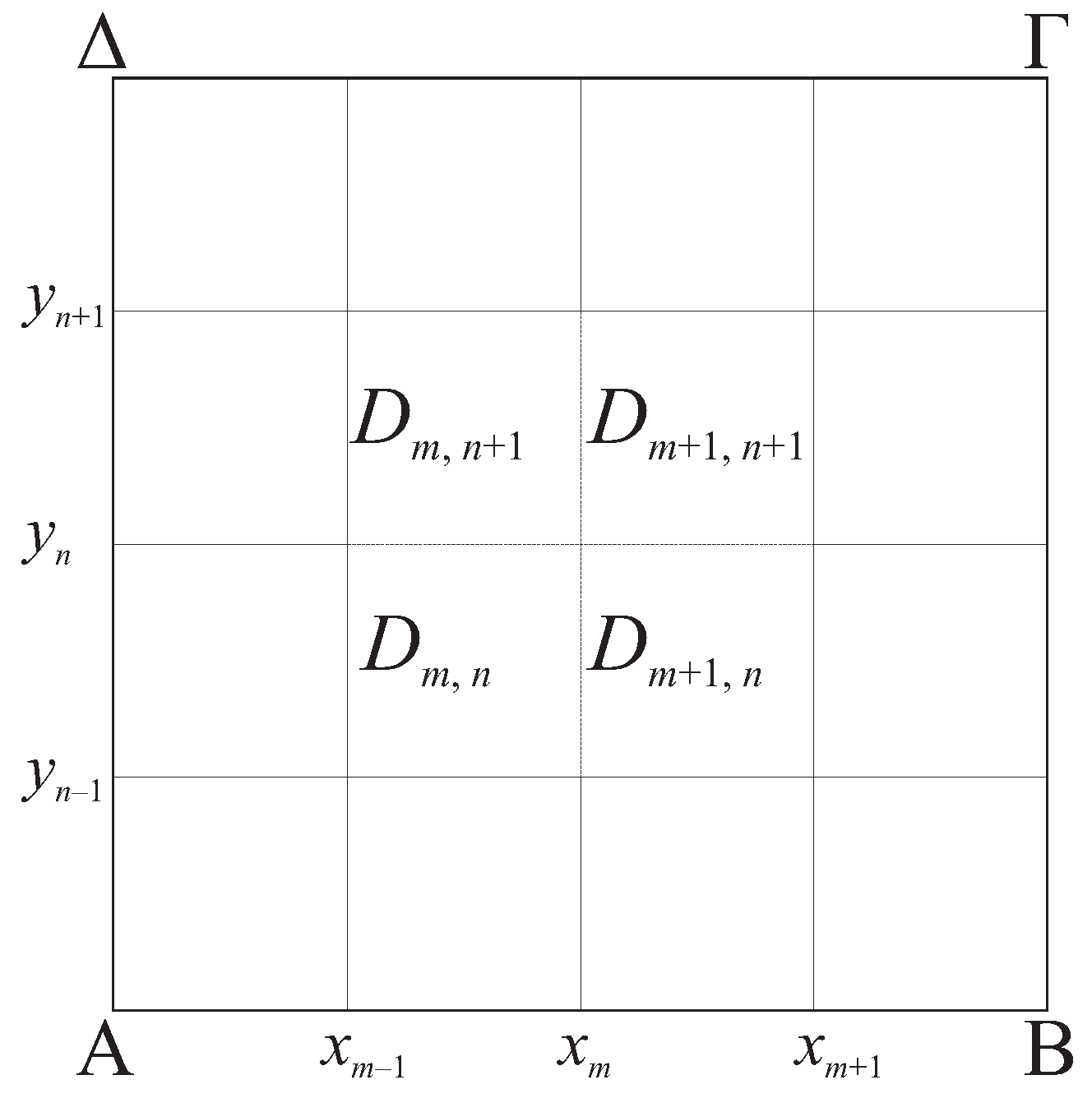
for any $f\in C_0\left(D\right)$, $(x,y)\in D_{m,n}$, $m=1,2,\dots ,M$ and $n=1,2,\dots ,N$. We verify that $\mathsf{\Phi }$ is well defined and that does indeed take $C_0\left(D\right)$ into itself. If $x\ne x_i$, $i=0,1,\dots ,M$ and $y\ne y_j$, $j=0,1,\dots ,N$, the value of $\mathsf{\Phi }\left(f\right)$ is uniquely determined by Equation (11). It remains to be demonstrated that $\mathsf{\Phi }\left(f\right)$ is well defined at the points $(x,y)$ which lie at the common boundaries of two or more subrectangles, say $D_{m,n}$ and $D_{m+1,n}$ as depicted in Figure 1, that is $x=x_m$ and $y_{n-1}\le y\le y_n$.

Observe first that due to Conditions (1), (3) and (10)

$$\begin{array}{c}{G}_{m,n}\left(L_{x_m}^{-1}\left(x_m\right),L_{y_n}^{-1}\left(y\right),f(L_{x_m}^{-1}\left(x_m\right),L_{y_n}^{-1}\left(y\right))\right)=G_{m,n}\left(x_M,L_{y_n}^{-1}\left(y\right),f(x_M,L_{y_n}^{-1}\left(y\right))\right)\hfill \\ =\left[F_{m,n}\left(x_M,L_{y_n}^{-1}\left(y\right),f(x_M,L_{y_n}^{-1}\left(y\right))\right)+F_{m+1,n}\left(x_0,L_{y_n}^{-1}\left(y\right),f(x_0,L_{y_n}^{-1}\left(y\right))\right)\right]/2\hfill \\ =\left[F_{m+1,n}\left(x_0,L_{y_n}^{-1}\left(y\right),f(x_0,L_{y_n}^{-1}\left(y\right))\right)+F_{m,n}\left(x_M,L_{y_n}^{-1}\left(y\right),f(x_M,L_{y_n}^{-1}\left(y\right))\right)\right]/2\hfill \\ =G_{m+1,n}\left(x_0,L_{y_n}^{-1}\left(y\right),f(x_0,L_{y_n}^{-1}\left(y\right))\right)=G_{m+1,n}\left(L_{x_{m+1}}^{-1}\left(x_m\right),L_{y_n}^{-1}\left(y\right),f(L_{x_{m+1}}^{-1}\left(x_m\right),L_{y_n}^{-1}\left(y\right))\right).\hfill \end{array}$$

Analogously, Condition (10) ensures the equivalence of the values of $\mathsf{\Phi }\left(f\right)$ along net segments $\{(x,y_n):x_{m-1}\le x\le x_m\}$. Therefore $\mathsf{\Phi }\left(f\right)$ is well defined on D. Moreover, the function $\mathsf{\Phi }\left(f\right)$ obeys the endpoint conditions because

$$\begin{array}{cc}\hfill \left(\mathsf{\Phi }f\right)(x_0,y_0)& =G_{1,1}\left(L_{x_1}^{-1}\left(x_0\right),L_{y_1}^{-1}\left(y_0\right),f(L_{x_1}^{-1}\left(x_0\right),L_{y_1}^{-1}\left(y_0\right))\right)=G_{1,1}(x_0,y_0,f(x_0,y_0))\hfill \\ & =F_{1,1}(x_0,y_0,f(x_0,y_0))=F_{1,1}(x_0,y_0,z_{0,0})=z_{0,0},\hfill \end{array}$$

$$\begin{array}{cc}\hfill \left(\mathsf{\Phi }f\right)(x_0,y_N)& =G_{1,N}\left(L_{x_1}^{-1}\left(x_0\right),L_{y_N}^{-1}\left(y_N\right),f(L_{x_1}^{-1}\left(x_0\right),L_{y_N}^{-1}\left(y_N\right))\right)=G_{1,N}(x_0,y_N,f(x_0,y_N))\hfill \\ & =F_{1,N}(x_0,y_N,f(x_0,y_N))=F_{1,N}(x_0,y_0,z_{0,N})=z_{0,N},\hfill \end{array}$$

$$\begin{array}{cc}\hfill \left(\mathsf{\Phi }f\right)(x_M,y_0)& =G_{M,1}\left(L_{x_M}^{-1}\left(x_M\right),L_{y_1}^{-1}\left(y_0\right),f(L_{x_M}^{-1}\left(x_M\right),L_{y_1}^{-1}\left(y_0\right))\right)=G_{M,1}(x_M,y_0,f(x_M,y_0))\hfill \\ & =F_{M,1}(x_M,y_0,f(x_M,y_0))=F_{M,1}(x_M,y_0,z_{M,0})=z_{M,0},\hfill \end{array}$$

and

$$\begin{array}{cc}\hfill \left(\mathsf{\Phi }f\right)(x_M,y_N)& =G_{M,N}\left(L_{x_1}^{-1}\left(x_M\right),L_{y_N}^{-1}\left(y_N\right),f(L_{x_1}^{-1}\left(x_M\right),L_{y_N}^{-1}\left(y_N\right))\right)=G_{M,N}(x_M,y_N,f(x_M,y_N))\hfill \\ & =F_{M,N}(x_M,y_N,f(x_M,y_N))=F_{M,N}(x_M,y_N,z_{M,N})=z_{M,N},\hfill \end{array}$$

which shows that $\mathsf{\Phi }\left(f\right)$ is well defined at each of the points $(x_i,y_j)$, $i=0,1,\dots ,M$ and $j=0,1,\dots ,N$. $L_{m,n}$ are continuous with continuous inverse, f is assumed continuous and $G_{m,n}$ are continuous, so $\mathsf{\Phi }$ is continuous on each of the compact sets $D_{m,n}$. Hence, indeed $\mathsf{\Phi }f\in C_0\left(D\right)$.

We now show that $\mathsf{\Phi }$ is a contraction on the metric space $(C_0\left(D\right),\rho )$. Let $f,g\in C_0\left(D\right)$ and $(x,y)\in D_{m,n}$, for $m=1,2,\dots ,M$ and $n=1,2,\dots ,N$. For $x=x_0$ we must select the third case of Condition (10). Then

$$\begin{array}{ccc}\rho \left(\mathsf{\Phi }f\right(x),\mathsf{\Phi }g(x\left)\right)\hfill & =\hfill & sup\left\{\right|\mathsf{\Phi }f(x,y)-\mathsf{\Phi }g(x,y)|:(x,y)\in D\}\hfill \\ & =\hfill & \underset{m,n}{max}sup\left\{\right|\mathsf{\Phi }f(x,y)-\mathsf{\Phi }g(x,y)|:(x,y)\in D_{m,n}\}\hfill \\ & =\hfill & \underset{m,n}{max}sup\left\{\right|G_{m,n}(x_0,L_{y_n}^{-1}\left(y\right),f(x_0,L_{y_n}^{-1}\left(y\right)))\hfill \\ & & -G_{m,n}(x_0,L_{y_n}^{-1}\left(y\right),g(x_0,L_{y_n}^{-1}\left(y\right)))|:y\in I_{y_n}\}\hfill \\ & =\hfill & \underset{m,n}{max}sup\left\{\right|[F_{m,n}(x_0,L_{y_n}^{-1}\left(y\right),f(x_0,L_{y_n}^{-1}\left(y\right)))+F_{m-1,n}(x_M,L_{y_n}^{-1}\left(y\right),f(x_M,L_{y_n}^{-1}\left(y\right)))]/2\hfill \\ & & -[F_{m,n}(x_0,L_{y_n}^{-1}\left(y\right),g(x_0,L_{y_n}^{-1}\left(y\right)))+F_{m-1,n}(x_M,L_{y_n}^{-1}\left(y\right),g(x_M,L_{y_n}^{-1}\left(y\right)))]/2|:y\in I_{y_n}\}\hfill \\ & =\hfill & \underset{m,n}{max}sup\left\{\right|[s_{m,n}\left(f(x_0,L_{y_n}^{-1}\left(y\right))-g(x_0,L_{y_n}^{-1}\left(y\right))\right)\hfill \\ & & +s_{m-1,n}\left(f(x_M,L_{y_n}^{-1}\left(y\right))-g(x_M,L_{y_n}^{-1}\left(y\right))\right)]/2|:y\in I_{y_n}\}\hfill \\ & \le \hfill & (1/2)\underset{m,n}{max}sup\left\{\right|s_{m,n}\left(f(x_0,L_{y_n}^{-1}\left(y\right))-g(x_0,L_{y_n}^{-1}\left(y\right))\right)|\hfill \\ & & +|s_{m-1,n}\left(f(x_M,L_{y_n}^{-1}\left(y\right))-g(x_M,L_{y_n}^{-1}\left(y\right))\right)|:y\in I_{y_n}\}\hfill \\ & \le \hfill & \underset{m,n}{max}|s_{m,n}|sup\{|f(x,y)-g(x,y)|:(x,y)\in D\}\hfill \\ & \le \hfill & s\rho \left(f\right(x),g(x\left)\right),\hfill \end{array}$$

where $s=max\left\{\right|s_{m,n}|:m=2,3\dots ,M-1;n=1,2,\dots ,N\}<1$. The proof is similar for the cases $x=x_M$, $y=y_0$ and $y=y_N$. Let $f,g\in C_0\left(D\right)$ and $(x,y)\in D_{m,n}$, for $m=2,3,\dots ,M-1$ and $n=2,3,\dots ,N-1$. Then

$$\begin{array}{ccc}\hfill \rho \left(\mathsf{\Phi }f\right(x),\mathsf{\Phi }g(x\left)\right)& =& sup\left\{\right|\mathsf{\Phi }f(x,y)-\mathsf{\Phi }g(x,y)|:(x,y)\in D\}\hfill \\ & =& \underset{m,n}{max}sup\left\{\right|\mathsf{\Phi }f(x,y)-\mathsf{\Phi }g(x,y)|:(x,y)\in D_{m,n}\}\hfill \\ & =& \underset{m,n}{max}sup\left\{\right|G_{m,n}(L_{x_m}^{-1}\left(x\right),L_{y_n}^{-1}\left(y\right),f(L_{x_m}^{-1}\left(x\right),L_{y_n}^{-1}\left(y\right)))\hfill \\ & & -G_{m,n}(L_{x_m}^{-1}\left(x\right),L_{y_n}^{-1}\left(y\right),g(L_{x_m}^{-1}\left(x\right),L_{y_n}^{-1}\left(y\right)))|:(x,y)\in D_{m,n}\}\hfill \\ & =& \underset{m,n}{max}sup\left\{\right|F_{m,n}(L_{x_m}^{-1}\left(x\right),L_{y_n}^{-1}\left(y\right),f(L_{x_m}^{-1}\left(x\right),L_{y_n}^{-1}\left(y\right)))\hfill \\ & & -F_{m,n}(L_{x_m}^{-1}\left(x\right),L_{y_n}^{-1}\left(y\right),g(L_{x_m}^{-1}\left(x\right),L_{y_n}^{-1}\left(y\right)))|:(x,y)\in D_{m,n}\}\hfill \\ & =& \underset{m,n}{max}sup\left\{\right|s_{m,n}[f(L_{x_m}^{-1}\left(x\right),L_{y_n}^{-1}\left(y\right))-g(L_{x_m}^{-1}\left(x\right),L_{y_n}^{-1}\left(y\right))]|:(x,y)\in D_{m,n}\}\hfill \\ & =& \underset{m,n}{max}|s_{m,n}|sup\{|f(x,y)-g(x,y)|:(x,y)\in D\}\hfill \\ & \le & s\rho \left(f\right(x),g(x\left)\right),\hfill \end{array}$$

where $s=max\left\{\right|s_{m,n}|:m=2,3\dots ,M-1;n=2,3,\dots ,N-1\}<1$. It follows that $\rho (\mathsf{\Phi }f,\mathsf{\Phi }g)\le s\rho (f,g)$ and we conclude that $\mathsf{\Phi }:C_0\left(D\right)\to C_0\left(D\right)$ is a contraction mapping.

The Contraction Mapping Theorem implies that $\mathsf{\Phi }$ possesses a unique fixed point in $C_0\left(D\right)$, namely

$$\left(\mathsf{\Phi }f\right)(x,y)=f(x,y)$$

or, equivalently,

$$G_{m,n}(x,y,f(x,y))=f\left(L_{m,n}(x,y)\right),$$

for all $(x,y)\in D$, $m=1,2,\dots ,M$ and $n=1,2,\dots ,N$.

Denote the unique attractor of $\{K;w_{1-M,1-N}\}$ by G. As we have mentioned before, $\{D;L_{1-M,1-N}\}$ is also a hyperbolic IFS whose unique attractor is D. The graph $\widehat{G}$ of f is also an attractor of $\{K;w_{1-M,1-N}\}$, for

$$\begin{array}{ccc}\hfill W\left(\widehat{G}\right)& =& \bigcup _{m=1}^M\bigcup _{n=1}^N{w}_{m,n}\left(\widehat{G}\right)=\bigcup _{m=1}^M\bigcup _{n=1}^N{w}_{m,n}\left(\{(x,y,f(x,y)):(x,y)\in D\}\right)\hfill \\ & =& \bigcup _{m=1}^M\bigcup _{n=1}^N\{(L_{m,n}(x,y),G_{m,n}(x,y,f(x,y))):(x,y)\in D\}\hfill \\ & =& \bigcup _{m=1}^M\bigcup _{n=1}^N\{(L_{m,n}(x,y),f\left(L_{m,n}(x,y)\right)):(x,y)\in D\}=\widehat{G}.\hfill \end{array}$$

Thus, the graph of f is an attractor for the IFS $\{K;w_{1-M,1-N}\}$ and so it must be equal to G. □

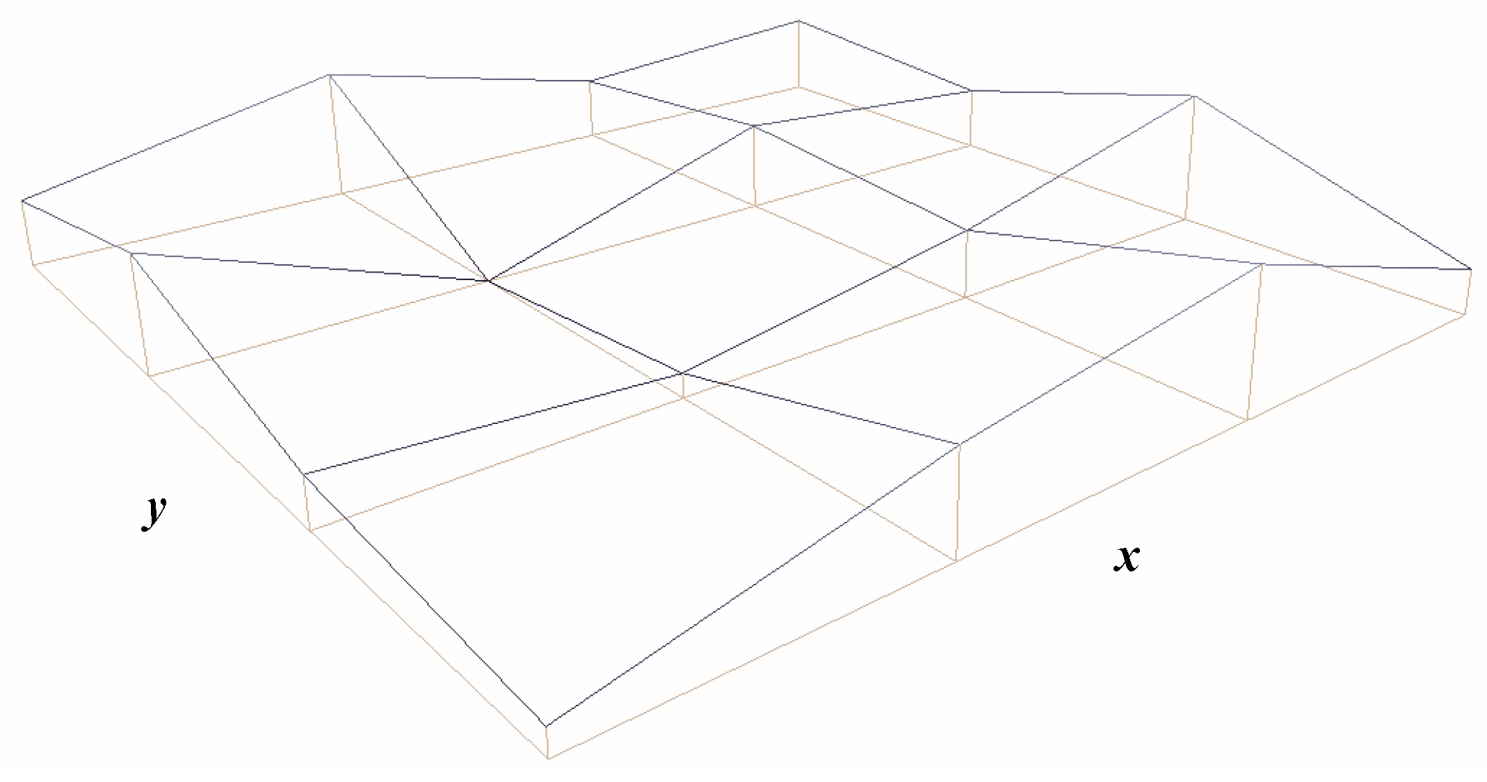
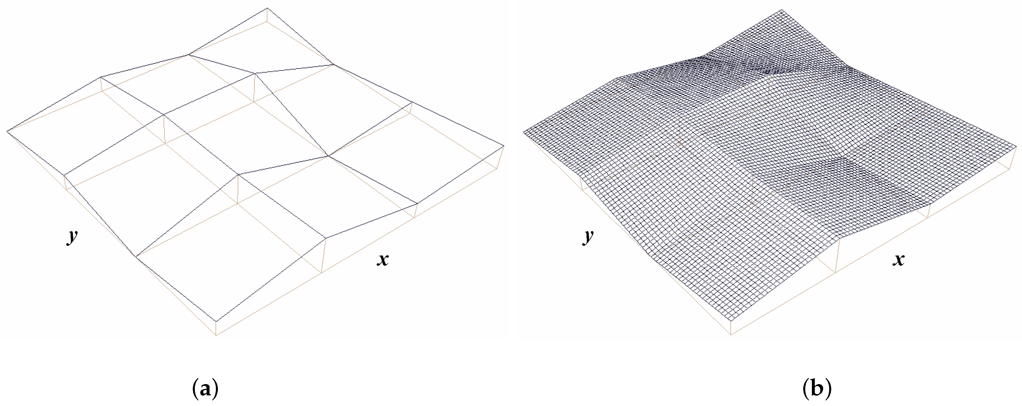
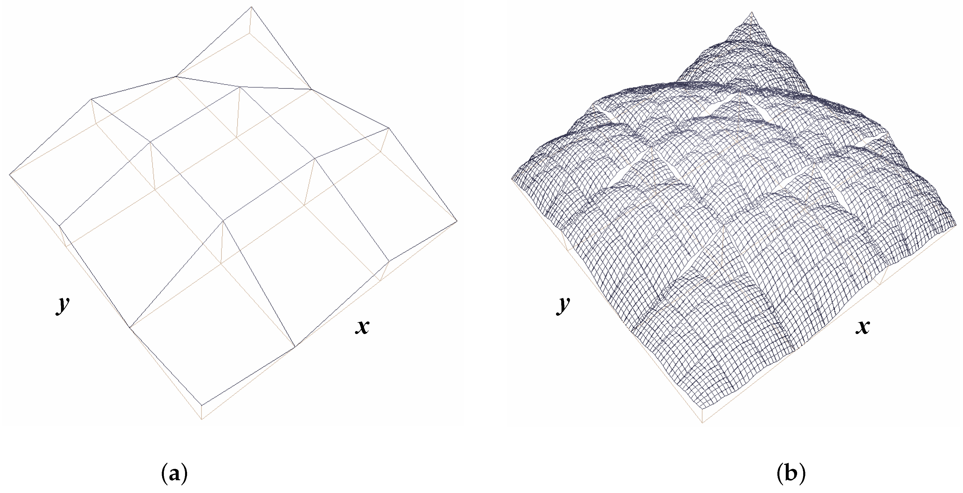
All of the figures are presented here to enable comparison of our general, in view of Equation (10), construction method against reference fractal surfaces. The method used for constructing these figures is based on the Deterministic Iteration Algorithm with various levels; see [2] for details. Figure 2 illustrates the surface graph (Level = 0) drawn with the original set of data given in Table 1 of [9]. Although the vertical scaling factors used for drawing Figure 5 of [9] are not given, we speculate that for Figure 5a $s_{m,n}=0.447207$ and for Figure 5b $s_{m,n}=0.59160$ for all $m=1,2,3$ and $n=1,2,3$ because of the quoted in [9] fractal dimension. In Figure 3a a fractal interpolated surface using Equation (13) of [9] is illustrated whereas in Figure 3b a fractal interpolation surface using our construction is illustrated, where $s_{m,n}=0.447207$ for all $m=1,2,3$, $n=1,2,3$ and Level = 4.

6. Other Constructions

6.1. On Continuity between Adjacent Subdomains

The key difficulty in constructing IFSs based on Equation (8) involves ensuring continuity. Adjacent subdomains are associated with different mappings and yet share common points. To guarantee continuity, we require that these adjacent mappings produce the same values at these common points. Referring to Figure 1, let $(x^{\prime },y^{\prime })$ be a point on the boundary of the adjacent subdomains $D_{m,n}$ and $D_{m+1,n}$, which are associated with the mappings $F_{m,n}$ and $F_{m+1,n}$, respectively. For the boundary point we have both $(x^{\prime },y^{\prime })\in D_{m,n}$ and $(x^{\prime },y^{\prime })\in D_{m+1,n}$, that is $x^{\prime }=x_m$ and $y_{n-1}\le y^{\prime }\le y_n$. With this in mind, we can see that for continuity it is required that

$$F_{m,n}\left(L_{x_m}^{-1}\left(x_m\right),L_{y_n}^{-1}\left(y^{\prime }\right),f(L_{x_m}^{-1}\left(x_m\right),L_{y_n}^{-1}\left(y^{\prime }\right))\right)=F_{m+1,n}\left(L_{x_{m+1}}^{-1}\left(x_m\right),L_{y_n}^{-1}\left(y^{\prime }\right),f(L_{x_{m+1}}^{-1}\left(x_m\right),L_{y_n}^{-1}\left(y^{\prime }\right))\right)$$

or

$$\begin{array}{c}\hfill F_{m,n}\left(x_M,L_{y_n}^{-1}\left(y^{\prime }\right),f(x_M,L_{y_n}^{-1}\left(y^{\prime }\right))\right)=F_{m+1,n}\left(x_0,L_{y_n}^{-1}\left(y^{\prime }\right),f(x_0,L_{y_n}^{-1}\left(y^{\prime }\right))\right).\end{array}$$

(12)

These requirements are sometimes referred to as the ‘join-up’ conditions.

We can rewrite Equation (7) as

$$\begin{array}{c}\hfill \frac{x^{\prime }-x_m}{x_m-x_{m-1}}=\frac{x-x_M}{{\Delta }_x},\frac{x^{\prime }-x_{m-1}}{x_m-x_{m-1}}=\frac{x-x_0}{{\Delta }_x},\frac{y^{\prime }-y_n}{y_n-y_{n-1}}=\frac{y-y_N}{{\Delta }_y},\frac{y^{\prime }-y_{n-1}}{y_n-y_{n-1}}=\frac{y-y_0}{{\Delta }_y}\end{array}$$

(13)

for $m=1,2,\dots ,M$ and $n=1,2,\dots ,N$. By using Equation (9) we get

$$\begin{array}{ccc}\hfill F_{m,n}\left(x_M,L_{y_n}^{-1}\left(y^{\prime }\right),f(x_M,L_{y_n}^{-1}\left(y^{\prime }\right))\right)& =& \frac{y^{\prime }-y_{n-1}}{y_n-y_{n-1}}{z}_{m,n}+\frac{y^{\prime }-y_n}{y_{n-1}-y_n}{z}_{m,n-1}\hfill \\ & & +s_{m,n}\left(z_{B\Gamma }-\frac{y^{\prime }-y_{n-1}}{y_n-y_{n-1}}{z}_{M,N}-\frac{y^{\prime }-y_n}{y_{n-1}-y_n}{z}_{M,0}\right),\hfill \end{array}$$

(14)

where $z_{B\Gamma }=f(x_M,y)$ and

$$\begin{array}{ccc}\hfill F_{m+1,n}\left(x_0,L_{y_n}^{-1}\left(y^{\prime }\right),f(x_0,L_{y_n}^{-1}\left(y^{\prime }\right))\right)& =& \frac{y^{\prime }-y_{n-1}}{y_n-y_{n-1}}{z}_{m,n}+\frac{y^{\prime }-y_n}{y_{n-1}-y_n}{z}_{m,n-1}\hfill \\ & & +s_{m+1,n}\left(z_{A\Delta }-\frac{y^{\prime }-y_{n-1}}{y_n-y_{n-1}}{z}_{0,N}-\frac{y^{\prime }-y_n}{y_{n-1}-y_n}{z}_{0,0}\right),\hfill \end{array}$$

(15)

where $z_{A\Delta }=f(x_0,y)$. In order for the join-up conditions (12) to be satisfied, we must have

$$\begin{array}{c}\hfill s_{m,n}\left(z_{B\Gamma }-\frac{y^{\prime }-y_{n-1}}{y_n-y_{n-1}}{z}_{M,N}-\frac{y^{\prime }-y_n}{y_{n-1}-y_n}{z}_{M,0}\right)=s_{m+1,n}\left(z_{A\Delta }-\frac{y^{\prime }-y_{n-1}}{y_n-y_{n-1}}{z}_{0,N}-\frac{y^{\prime }-y_n}{y_{n-1}-y_n}{z}_{0,0}\right)\end{array}$$

or, by using (13),

$$\begin{array}{c}\hfill s_{m,n}\left(z_{B\Gamma }-\frac{y-y_0}{{\Delta }_y}{z}_{M,N}+\frac{y-y_N}{{\Delta }_y}{z}_{M,0}\right)=s_{m+1,n}\left(z_{A\Delta }-\frac{y-y_0}{{\Delta }_y}{z}_{0,N}+\frac{y-y_N}{{\Delta }_y}{z}_{0,0}\right).\end{array}$$

Similarly, if $(x^{\prime },y^{\prime })$ is a point on the boundary of the adjacent subdomains $D_{m,n}$ and $D_{m,n+1}$, which are associated with the mappings $F_{m,n}$ and $F_{m,n+1}$, respectively, we have that

$$\begin{array}{c}\hfill s_{m,n}\left(z_{\Delta \Gamma }-\frac{x-x_0}{{\Delta }_x}{z}_{M,N}+\frac{x-x_M}{{\Delta }_x}{z}_{0,N}\right)=s_{m,n+1}\left(z_{AB}-\frac{x-x_0}{{\Delta }_x}{z}_{M,0}+\frac{x-x_M}{{\Delta }_x}{z}_{0,0}\right),\end{array}$$

where $z_{\Delta \Gamma }=f(x,y_N)$ and $z_{AB}=f(x,y_0)$. The last two equations can be written in the form

$$\begin{array}{c}\hfill s_{m,n}\left(z_{B\Gamma }+q_1\left(y\right)\right)=s_{m+1,n}\left(z_{A\Delta }+q_0\left(y\right)\right)\mathrm{and}{s}_{m,n}\left(z_{\Delta \Gamma }+p_1\left(x\right)\right)=s_{m,n+1}\left(z_{AB}+p_0\left(x\right)\right)\end{array}$$

according to Qian’s notation. Note that $q_1\left(y\right)\equiv f^r\left(y\right)$, $q_0\left(y\right)\equiv f^l\left(y\right)$, $p_1\left(x\right)\equiv f^o\left(x\right)$ and $p_0\left(x\right)\equiv f^u\left(x\right)$ according to Feng’s notation and that $z_{AB}\equiv z_{i,0}$, $z_{B\Gamma }\equiv z_{M,j}$, $z_{\Delta \Gamma }\equiv z_{i,N}$ and $z_{A\Delta }\equiv z_{0,j}$ for all $i=0,1,\dots ,M$ and $j=0,1,\dots ,N$ if we consider the self-affinity of the resulting surface. Combining the two equations we obtain that the attractor G will be the graph of a continuous function $f:D\to \mathbb{R}$, if one of the following conditions is fulfilled:

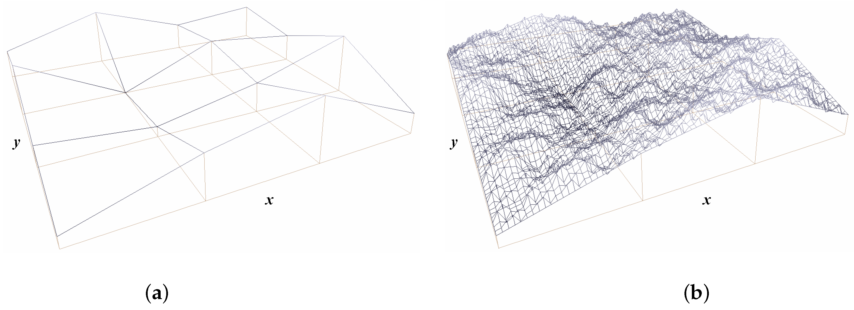
($\alpha$) All vertical scaling factors vanish. If $s_{m,n}=0$ for all $m=1,2,\dots ,M$ and $n=1,2,\dots ,N$, the join-up conditions are automatically satisfied. Figure 4a illustrates the surface graph (Level = 0) drawn with the original set of data given in Figure 2 of [30]. In Figure 4b a (fractal) interpolation surface using the standard, in view of Equation (8), bivariate construction is illustrated, where $s_{m,n}=0.0$ for all $m=1,2,3$, $n=1,2,3$ and Level = 4.

($\beta$) All interpolating nodes of the sides AB, B$\Gamma ,\Gamma \Delta$ and $\Delta$A of Figure 1 are collinear. This summarizes the work of Leoni Dalla and Hong-Yong Wang. If

$$z_{B\Gamma }=\frac{y-y_0}{{\Delta }_y}{z}_{M,N}-\frac{y-y_N}{{\Delta }_y}{z}_{M,0},z_{A\Delta }=\frac{y-y_0}{{\Delta }_y}{z}_{0,N}-\frac{y-y_N}{{\Delta }_y}{z}_{0,0}$$

and

$$z_{\Delta \Gamma }=\frac{x-x_0}{{\Delta }_x}{z}_{M,N}-\frac{x-x_M}{{\Delta }_x}{z}_{0,N},z_{AB}=\frac{x-x_0}{{\Delta }_x}{z}_{M,0}-\frac{x-x_M}{{\Delta }_x}{z}_{0,0},$$

the interpolation points on each edge of the rectangular grid are collinear. Figure 5a illustrates the surface graph (Level = 0) drawn with the original set of data given in

Table 1. The original data for fractal interpolating surface (a) of Condition $\beta$ and (b) of Condition $\gamma$(i).

	x	0	1	2	3		x	0	1	2	3
y						y
0		0.1	0.2	0.3	0.4	0		0.1	0.2	0.3	0.4
1		0.3	0.1	0.3	0.4	1		0.5	0.1	0.4	0.8
2		0.5	0.0	0.4	0.4	2		0.3	0.2	0.5	0.6
3		0.7	0.6	0.5	0.4	3		0.4	0.5	0.6	0.7
(a)						(b)

a. In Figure 5b a fractal interpolation surface using the standard, in view of Equation (8), bivariate construction is illustrated, where $s_{1,1}=s_{3,1}=s_{2,2}=s_{3,3}=0.40$, $s_{1,2}=s_{2,1}=s_{3,2}=-s_{2,3}=0.30$, $s_{1,3}=0.20$ and Level = 4.

($\gamma$) All interpolating nodes of the sides AB and B$\Gamma$ of Figure 1 are transformed images of the corresponding nodes of $\Gamma \Delta$ and $\Delta$A. The following subcases are worth mentioning:

(i) If $s_{m,n}=s_{m+1,n}$ for all $m=1,2,\dots ,M-1$ and $n=1,2,\dots ,N$, not all identically zero, $z_{\Delta \Gamma }+p_1\left(x\right)=z_{AB}+p_0\left(x\right)=0$ and $z_{B\Gamma }+q_1\left(y\right)=z_{A\Delta }+q_0\left(y\right)$, the join-up conditions are satisfied. This means that there is no need for collinear boundary data on B$\Gamma$ and $\Delta$A; see Figure 1. Figure 6a is the surface graph (Level = 0) drawn with the original set of data given in Table 1b. In Figure 6b a fractal interpolation surface using the standard, in view of Equation (8), bivariate construction is illustrated, where $s_{1,1}=s_{2,1}=s_{3,1}=0.50$, $s_{1,2}=s_{2,2}=s_{3,2}=0.40$, $s_{1,3}=s_{2,3}=s_{3,3}=0.30$ and Level = 4.

(ii) If $s_{m,n}=s_{m,n+1}$ for all $m=1,2,\dots ,M$ and $n=1,2,\dots ,N-1$, not all identically zero, $z_{B\Gamma }+q_1\left(y\right)=z_{A\Delta }+q_0\left(y\right)=0$ and $z_{\Delta \Gamma }+p_1\left(x\right)=z_{AB}+p_0\left(x\right)$, the join-up conditions are satisfied. This means that there is no need for collinear boundary data on AB and $\Gamma \Delta$; see Figure 1.

(iii) All interpolating nodes on the sides AB and B$\Gamma$ are reflected on $\Gamma \Delta$ and $\Delta$A of Figure 1, respectively. If $z_{0,j}=z_{M,j},j=0,1,\dots ,N$, $z_{i,0}=z_{i,N},i=0,1,\dots ,M$ and $s_{m,n}=s$ for all $m=1,2,\dots ,M$ and $n=1,2,\dots ,N$ the join-up conditions are satisfied. Figure 7a is the surface graph (Level = 0) drawn with the original set of data given in

Table 2. (a) The original data used for the fractal surface. (b) The data used for the general construction.

	x	0	1	2	3	4		x	0	1	2	3	4	5
y							y
0		0.1	0.0	0.6	0.2	0.1	0		0.0	0.1	0.2	0.3	0.4	0.5
1		0.2	0.0	0.0	0.6	0.2	1		0.0	0.1	0.4	0.6	0.2	0.5
2		0.5	0.0	0.2	0.4	0.5	2		0.0	0.2	0.1	0.3	0.6	0.5
3		0.3	0.3	0.3	0.5	0.3	3		0.0	0.5	0.0	0.4	0.3	0.5
4		0.1	0.0	0.6	0.2	0.1	4		0.0	0.3	0.6	0.3	0.4	0.5
							5		0.0	0.1	0.2	0.3	0.4	0.5
(a)							(b)

a. In Figure 7b a fractal interpolation surface using the standard, in view of Equation (8), bivariate construction is illustrated, where $s_{m,n}=0.4$ for all $m=1,2,3,4$, $n=1,2,3,4$ and Level = 4.

($\delta$) We allow the contractivity factors to become a continuous ‘contraction function’ as shown in Nailiang Zhao’s paper and also consider reflections as shown in Jeffery R. Price and Monson H. Hayes III paper.

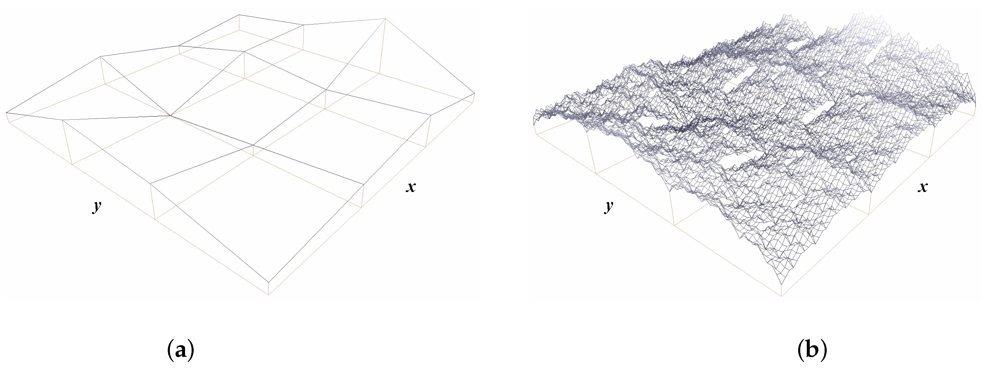
Figure 8a illustrates the surface graph (Level = 0) drawn with the original set of data given in Figure 3 of [30]. In Figure 8b a fractal surface using the standard, in view of Equation (8), bivariate construction is illustrated, where $s_{m,n}=0.30$ for all $m=1,2,3$, $n=1,2,3$ and Level = 4. In this example, the obtained interpolant is not continuous because neither of the conditions for obtaining the continuous interpolant is satisfied.

6.2. Remarks and Examples

6.2.1. Leoni Dalla’s work

The central part of this construction is based on the assumption that the interpolation points on each edge of the rectangular grid are collinear. So, paraphrasing Condition (*) mentioned in [14] and using our notation, each one of the sets

$$\begin{array}{ccc}\hfill \{(x_0,y_j,z_{0,j}):j=0,1,\dots ,N\},& & \{(x_M,y_j,z_{M,j}):j=0,1,\dots ,N\},\hfill \\ \hfill \{(x_i,y_0,z_{i,0}):i=0,1,\dots ,M\},& & \{(x_i,y_N,z_{i,N}):i=0,1,\dots ,M\}\hfill \end{array}$$

(16)

is collinear. For instance, collinearity of the set $\{(x_M,y_j,z_{M,j}):j=0,1,\dots ,N\}$ means that $x=x_M$, $y=y_0+t{\Delta }_y=t{y}_N+(1-t)y_0$, $z=z_{M,0}+t(z_{M,N}-z_{M,0})=t{z}_{M,N}+(1-t)z_{M,0}$ for all $t\in [0,1]$. She used the above-mentioned condition in order to prove, in Prop. 2.2, that the function $\mathsf{\Phi }\left(f\right)$ obeys the conditions

$$\begin{array}{ccc}\hfill \mathsf{\Phi }f(x_0,(1-\lambda )y_0+\lambda y_N)& =& (1-\lambda )z_{0,0}+\lambda z_{0,N}\hfill \\ \hfill \mathsf{\Phi }f(x_M,(1-\lambda )y_0+\lambda y_N)& =& (1-\lambda )z_{M,0}+\lambda z_{M,N}\hfill \\ \hfill \mathsf{\Phi }f((1-\lambda )x_0+\lambda x_M,y_0)& =& (1-\lambda )z_{0,0}+\lambda z_{M,0}\hfill \\ \hfill \mathsf{\Phi }f((1-\lambda )x_0+\lambda x_M,y_N)& =& (1-\lambda )z_{0,M}+\lambda z_{M,N}\hfill \end{array}$$

for all $\lambda \in [0,1]$.

Note, that one must be careful when using the parameter $\lambda$, because Condition (7) can also be seen as

$$x^{\prime }={\lambda }_1{x}_m+(1-{\lambda }_1)x_{m-1},y^{\prime }={\lambda }_2{y}_n+(1-{\lambda }_2)y_{n-1},$$

where ${\lambda }_1\equiv {\lambda }_1\left(x\right)=(x-x_0)/{\Delta }_x$, ${\lambda }_2\equiv {\lambda }_2\left(y\right)=(y-y_0)/{\Delta }_y$ and ${\lambda }_1,{\lambda }_2\in [0,1]$. Therefore, $L_{x_m}^{-1}\left(x^{\prime }\right)=(1-{\lambda }_1)x_0+{\lambda }_1{x}_M$ and $L_{y_n}^{-1}\left(y^{\prime }\right)=(1-{\lambda }_2)y_0+{\lambda }_2{y}_N$ as opposed to the single parameter $\lambda$ mentioned before. To complete the proof on p. 57,

$$\begin{array}{ccc}\mathsf{\Phi }f(x_M,(1-{\lambda }_2)y_{n-1}+{\lambda }_2{y}_n)\hfill & =\hfill & F_{M,n}\left(L_{x_M}^{-1}\left(x_M\right),L_{y_n}^{-1}\left(y^{\prime }\right),f(L_{x_m}^{-1}\left(x_M\right),L_{y_n}^{-1}\left(y^{\prime }\right))\right)\hfill \\ & =\hfill & F_{M,n}\left(x_M,(1-{\lambda }_2)y_0+{\lambda }_2{y}_N,f(x_M,(1-{\lambda }_2)y_0+{\lambda }_2{y}_N)\right)\hfill \\ & =\hfill & s_{M,n}f(x_M,(1-{\lambda }_2)y_0+{\lambda }_2{y}_N)+h_{M,n}(x_M,(1-{\lambda }_2)y_0+{\lambda }_2{y}_N)\hfill \\ & =\hfill & s_{M,n}[(1-{\lambda }_2)z_{M,0}+{\lambda }_2{z}_{M,N}]+(1-{\lambda }_2)h_{M,n}(x_M,y_0)+{\lambda }_2{h}_{M,n}(x_M,y_N)\hfill \\ & =\hfill & (1-{\lambda }_2)[s_{M,N}{z}_{M,0}+h_{M,n}(x_M,y_0)]+{\lambda }_2[s_{M,n}{z}_{M,N}+h_{M,n}(x_M,y_N)]\hfill \\ & =\hfill & (1-{\lambda }_2)z_{M,n-1}+{\lambda }_2{z}_{M,n}\hfill \end{array}$$

using the fact that

$$\begin{array}{ccc}{h}_{M,n}(x_M,(1-{\lambda }_2)y_0+{\lambda }_2{y}_N)\hfill & =\hfill & e_{M,n}{x}_M+f_{M,n}[(1-{\lambda }_2)y_0+{\lambda }_2{y}_N]+g_{M,n}{x}_M[(1-{\lambda }_2)y_0+{\lambda }_2{y}_N]+k_{M,n}\hfill \\ & =\hfill & e_{M,n}{x}_M+(1-{\lambda }_2)f_{M,n}{y}_0+{\lambda }_2{f}_{M,n}{y}_N\hfill \\ & & +(1-{\lambda }_2)g_{M,n}{x}_M{y}_0+{\lambda }_2{g}_{M,n}{x}_M{y}_N+k_{M,n}\hfill \\ & =\hfill & {\lambda }_2(e_{M,n}{x}_M+f_{M,n}{y}_N+g_{M,n}{x}_M{y}_N+k_{M,n})\hfill \\ & & +(1-{\lambda }_2)(e_{M,n}{x}_M+f_{M,n}{y}_0+g_{M,n}{x}_M{y}_0+k_{M,n})\hfill \\ & =\hfill & (1-{\lambda }_2)h_{M,n}(x_M,y_0)+{\lambda }_2{h}_{M,n}(x_M,y_N)\hfill \end{array}$$

for all $n=1,2,\dots ,N$.

Despite these, she gave some figures, constructed by the first author, using noncollinear interpolation points. Those figures are not based on the general construction presented in Section 2.2 of [14]. Also, the data used for constructing the figures presented there are not given, although the initial purpose was to construct a bivariate fractal surface with the data given in Heping Xie and Hongquan Sun’s paper. Actually, Fig. 1 and Fig. 2 of [14] are based on the Condition $\gamma$(iii) of the previous subsection and the data used are given in Table 2a. Figure 9a is the surface graph (Level = 0) drawn with the original set of data given in Table 2b excluding the first and the last row as well the first and the last column. In Figure 9b a fractal interpolation surface using the general construction (Subsection 2.2 of [14]) is illustrated, where $s_{m,n}=0.4$ for all $m=1,2,3,4$, $n=1,2,3,4$ and Level = 3.

6.2.2. Qian’s Work

Among other things, a negative result concerning the existence of affine fractal interpolation functions defined on rectangular domains can also be found there. Lemma 4.2 of [16] follows from Condition ($\gamma$) of the previous subsection as a partial case because of the use of the same contractivity factor. Figure 10a illustrates the surface graph (Level = 0) drawn with the original set of data given in

Table 3. The interpolated data (a) of Qian’s work and (b) of Wang’s work.

	x	0	1	2		x	0	1	2	3	4	5
y					y
0		0.0	0.0	0.0	0		0.0	0.1	0.2	0.3	0.4	0.5
1		0.0	1.0	0.0	1		0.0	0.1	0.2	0.3	0.1	0.5
2		0.0	0.0	0.0	2		0.0	0.3	0.1	0.2	0.6	0.5
					3		0.0	0.4	0.0	0.3	0.3	0.5
					4		0.0	0.1	0.3	0.1	0.2	0.5
					5		0.0	0.1	0.2	0.3	0.4	0.5
(a)					(b)

a.

In Figure 10b a bivariate fractal interpolation surface using the standard, in view of Equation (8), construction is illustrated, where $s_{m,n}=0.4$ for all $m=1,2$, $n=1,2$ and Level = 5; see also Example 4.1 of [16] and Example 1 of [19].

6.2.3. Wang’s Work

This construction uses the same assumption with that of Dalla’s (p. 224) in order to prove that the function $\mathsf{\Phi }f$ of Theorem 2 of [18] obeys the following conditions presented on p. 225

$$\begin{array}{ccc}\hfill \mathsf{\Phi }f(x_0,(1-\lambda )y_0+\lambda y_N)& =& (1-\lambda )z_{0,0}+\lambda z_{0,N}\hfill \\ \hfill \mathsf{\Phi }f(x_M,(1-\lambda )y_0+\lambda y_N)& =& (1-\lambda )z_{M,0}+\lambda z_{M,N}\hfill \\ \hfill \mathsf{\Phi }f((1-\lambda )x_0+\lambda x_M,y_0)& =& (1-\lambda )z_{0,0}+\lambda z_{M,0}\hfill \\ \hfill \mathsf{\Phi }f((1-\lambda )x_0+\lambda x_M,y_N)& =& (1-\lambda )z_{0,M}+\lambda z_{M,N}\hfill \end{array}$$

for all $\lambda \in [0,1]$.

Moreover, the example mentioned on p. 226 consists of noncollinear interpolation points, but there is a reference to the general construction of Dalla. However, Figure 1 of [18] does not agree with the interpolated data given there. Figure 11a is the surface graph (Level = 0) drawn with the original set of data given in Table 1 of [18]. Figure 11b illustrates the bivariate fractal interpolation surface drawn with the original set of data given in Table 1 of [18] by using the standard, in view of Equation (8), construction, where $s_{m,n}=0.50$ for all $m=1,2,3$, $n=1,2,3$ and Level = 4.

Figure 12a illustrates the bivariate fractal interpolation surface drawn with the set of data given in Table 3b by using the general construction of Leoni Dalla, where $s_{m,n}=0.50$ for all $m=1,2,3$, $n=1,2,3$ and Level = 4. Figure 12b illustrates the bivariate fractal interpolation surface drawn with the original set of data given in Table 1 of [18] by using our construction, where $s_{m,n}=0.50$ for all $m=1,2,3$, $n=1,2,3$ and Level = 4.

6.2.4. Feng’s Work

Theorem 2.2 of [20], although not cited therein, is similar to Theorem 2.1 of [16] and gives necessary and sufficient conditions for the invariant set of an appropriately chosen IFS to be the graph of a continuous surface. However, continuity is not guaranteed for arbitrary interpolation points. Figure 13a is the surface graph (Level = 0) drawn with the original set of data given in Example 2.1 of [20]. In Figure 13b a fractal interpolation surface using the standard, in view of Equation (8), bivariate construction is illustrated, where $s_{m,n}=0.3$ for all $m=1,2,3,4$, $n=1,2,3$ and Level = 4.

7. Conclusions and Further Work

A method based on [9] for generating fractal interpolation surfaces was presented. The proposed function satisfies conditions similar to the so-called Dirichlet conditions, i.e., it is equal to the original function at points of continuity or to the average of the two limits at points of discontinuity. Necessary conditions for the attractor of an iterated function system to be the graph of a continuous bivariable function which interpolates a given set of data are also presented here. Moreover, a comparative study for the most important constructions and attempts on rectangular grids has been considered which has pointed out some of their limitations and restrictions. The methods presented here can be directly extended to piecewise fractal interpolation functions that are based on Recurrent IFS. A premise for future work is to extend these methods to hidden-variable fractal interpolation surfaces as well as to identify the parameters of such surfaces.

References

Barnsley, M.F. Fractal functions and interpolation. Constr. Approx.1986, 2, 303–329. [Google Scholar] [CrossRef]
Barnsley, M.F. Fractals Everywhere, 3rd ed.; Dover Publications, Inc.: New York, NY, USA, 2012. [Google Scholar]
Geronimo, J.S.; Hardin, D. Fractal interpolation surfaces and a related 2-D multiresolution analysis. J. Math. Anal. Appl.1993, 176, 561–586. [Google Scholar] [CrossRef][Green Version]
Hardin, D.P.; Massopust, P.R. Fractal interpolation functions from ℝn→ℝm and their projections. Z. Anal. Anwend.1993, 12, 535–548. [Google Scholar] [CrossRef]
Wittenbrink, C.M. IFS Fractal Interpolation for 2D and 3D Visualization. In Proceedings of the 6th IEEE Visualization Conference, Atlanta, GA, USA, 29 October–3 November 1995; pp. 77–84. [Google Scholar]
Zhao, N. Construction and application of fractal interpolation surfaces. Vis. Comput.1996, 12, 132–146. [Google Scholar] [CrossRef]
Massopust, P.R. Fractal Functions, Fractal Surfaces and Wavelets; Academic Press: San Diego, CA, USA, 1994. [Google Scholar]
Xie, H.; Sun, H. The study on bivariate fractal interpolation functions and creation of fractal interpolated surfaces. Fractals1997, 5, 625–634. [Google Scholar] [CrossRef]
Xie, H.; Sun, H. The theory of fractal interpolated surfaces and its applications. Appl. Math. Mech.1998, 19, 321–331. [Google Scholar] [CrossRef]
Price, J.R.; Hayes, M.H. Fractal interpolation of images and volumes. In Proceedings of the 32nd Asilomar Conference on Signals, Systems and Computers, Pacific Grove, CA, USA, 1–4 November 1998; Volume 2, pp. 1698–1702. [Google Scholar]
Xie, H.; Feng, Z. On star product fractal surfaces and their dimensions. Appl. Math. Mech.1999, 20, 1183–1189. [Google Scholar] [CrossRef]
Xie, H.; Sun, H.; Ju, Y.; Feng, Z. Study on generation of rock fracture surfaces by using fractal interpolation. Int. J. Solids Struct.2001, 38, 5765–5787. [Google Scholar] [CrossRef]
Dalla, L. Bivariate fractal interpolation functions on grids. Fractals2002, 10, 53–58. [Google Scholar] [CrossRef]
Kobes, R.; Penner, A.J. Nonlinear fractal interpolating functions of one and two variables. Fractals2005, 13, 179–186. [Google Scholar] [CrossRef]
Qian, X.Y. Bivariate fractal interpolation functions on rectangular domains. J. Comp. Math.2002, 20, 349–362. [Google Scholar]
Sun, H.; Xie, H. Study on the improved fractal interpolation surface of the attitude and surface fault. In Thinking in Patterns; Novak, M.M., Ed.; World Scientific: Singapore, 2004; pp. 243–254. [Google Scholar]
Wang, H.Y. On smoothness for a class of fractal interpolation surfaces. Fractals2006, 14, 223–230. [Google Scholar] [CrossRef]
Małysz, R. The Minkowski dimension of the bivariate fractal interpolation surfaces. Chaos Solitons Fractals2006, 27, 1147–1156. [Google Scholar] [CrossRef]
Feng, Z. Variation and Minkowski dimension of fractal interpolation surface. J. Math. Anal. Appl.2008, 345, 322–334. [Google Scholar] [CrossRef][Green Version]
Metzler, W.; Yun, C. Construction of fractal interpolation surfaces on rectangular grids. Int. J. Bifurc. Chaos2010, 20, 4079–4086. [Google Scholar] [CrossRef]
Wang, H.Y.; Ji, J.B. Surface fitting and error analysis using fractal interpolation. Int. J. Bifurc. Chaos2012, 22, 1250194. [Google Scholar] [CrossRef]
Ji, J.; Peng, J. Analytical properties of bivariate fractal interpolation functions with vertical scaling factor functions. Int. J. Comput. Math.2013, 90, 539–553. [Google Scholar] [CrossRef]
Ri, S. Nonlinear bivariate fractal interpolation function on grids. Chaos Solitons Fractals2015, 81, 351–358. [Google Scholar] [CrossRef]
Ri, S. A new construction of the fractal interpolation surface. Fractals2015, 23, 1550043. [Google Scholar] [CrossRef]
Okazaki, H.; Ueno, S.; Nakano, H. A bivariate fractal interpolation surface with an individual vertical scaling factor. In Proceedings of the 2016 IEEE International Symposium on Circuits and Systems (ISCAS), Montreal, QC, Canada, 22–25 May 2016; pp. 686–689. [Google Scholar]
Ri, S.I. A new nonlinear bivariate fractal interpolation function. Fractals2018, 26, 1850054. [Google Scholar] [CrossRef]
Ri, S. New types of fractal interpolation surfaces. Chaos Solitons Fractals2019, 119, 291–297. [Google Scholar] [CrossRef]